Land Use Change and Global Adaptations to Climate Change

Abstract

This paper uses the World Trade Model with Climate Sensitive Land (WTMCL) to evaluate possible future land-use changes associated with adaptations to climate change in a globalized world. In this approach, changes in regional agricultural production, which are based on comparative advantage, define patterns of land use change in agriculture in all regions of the world. We evaluate four scenarios that combine assumptions about future increases in food demand and future changes in land endowments of different productivities associated with climatic conditions: each scenario generates distinct patterns of regional specialization in the production of agricultural commodities and associated land-use change. The analysis also projects future food availability under the simulated conditions and the direction of likely changes in prices of the major agricultural commodity groups.

1. Introduction

Global studies of the impacts of climate change on agriculture and the role of trade as an adaptive mechanism anticipate that food availability will not be jeopardized for the next century or so [1,2,3,4,5]. These conclusions rely on model specifications that assume that a well-functioning system of trade, responsive to price signals, should shift commodity production to regions where comparative advantage for agricultural production improves under climate change, compensating for potential productivity losses in other regions of the world. Some results also rely on the (positive) fertilization effect that higher concentrations of atmospheric CO₂ could have on major cultivated crops. Recent field work, however, has raised doubts about the likelihood of such adjustments [6], enhancing the importance of an open system of trade in meeting future global food demand in the presence of climate change.

The magnitude of compensating changes in trade flows reported by most of these studies depend not only on the particular climate change assumptions, but also on the social and economic conditions embodied in their scenarios, such as increases in demand associated with population growth. To isolate the effects of climate change alone, Juliá and Duchin [1] analyzed climate change scenarios under constant (benchmark) socio-economic conditions; they found that, while the negative effects of climate change on land productivity could be compensated by trade adjustments, global prices of the agricultural commodities increased, as did the area of global cropland that would need to be cultivated. These results raise concerns about the long-term reliance on trade adaptations of agricultural systems to climate change, given that changes in both social expectations and economic conditions are likely to exceed the assumptions that underlie climate change projections [7], compounding the pressure on already scarce cropland.

The shortage of cropland to expand food production has been a topic of growing concern over the past decade. Tropical developing nations in particular are confronted by foreign acquisition of land often involving consolidation of small parcels, conversion from other uses, and deforestation [8]. During the 1980–2000 period, for example, more than half of the new agricultural land across the tropics came at the expense of intact forests, and another 28% came from disturbed forests [9]. Notions about adaptations to climate change generally presume an open system of trade in which global markets (and policies) influence opportunities and constraints on uses of land. Biophysical events such as climate change reshape the impacts of drivers of land allocation decisions, increasing the complexity of future pathways of land use change. These complexities need to be conceptualized as the basis for models used to project possible future paths and conclusions drawn from their results [10].

Most global models used to analyze future land-use associated with adaptations to climate change make use of Armington trade elasticities to regulate the extent of exchanges among trading partners. Similarly, they employ constant elasticities of transformation to govern the ease with which land moves across alternative uses. An important drawback of trade elasticities is that they take existing trade patterns, rather than ones based on comparative advantage, as their starting point; consequently, countries continue to import from virtually all the same sources even when regional production conditions change radically [1]. In addition, the value assigned to the land elasticity parameter cannot be measured directly and is (at best) inferred from relationships that held in other times and places [11] rather than letting factors such as projected gains or losses in productivity related to changing climatic conditions determine the optimal uses of land.

This paper describes a modeling approach—the World Trade Model with Climate Sensitive Land (WTMCL) [1]—which can be used to evaluate possible pathways of land-use change in response to the future demand for agricultural commodities in the presence of climate change. The model is specified as an open economic system of trade that allows global adaptations to drive land allocation decisions. Regional specialization in agricultural production—and associated patterns of land use—are determined by comparative advantage as influenced by growth in demand and changing climatic conditions, rather than exogenous elasticity values. Four scenarios represent future increases in population and associated demand for food in the presence and absence of climate change and accord producers the ability or not to convert land currently under forest. The analysis focuses on the likely locations and magnitude of agricultural production and related changes in land use and in prices. The next section presents the modeling framework and describes the scenarios. Section 3 reports the results of the scenario runs, and the final section summarizes and discusses the results.

2. Methods

2.1. Modeling Framework

The WTMCL model takes the form of a linear optimization problem that integrates a fully generalized system of trade based on comparative advantage for m regions, n goods and k factors, Duchin’s World Trade Model [12], with the spatial analogues approach of Darwin et al. [13], which quantifies climatic responses of land resources under alternative climate assumptions.

The spatial analogues approach defines a region’s climate in terms of its mean monthly temperature and precipitation. These variables define the region’s length of growing season (LGS), the longest continuous period of time in a year that soil temperature and moisture conditions support plant growth. Land resources are classified according to their LGS and the number of days with soil temperature above 5 °C, two climatically defined variables that correlate closely with agricultural productivity. Under this formulation, a change in climatic conditions affects a region’s endowments of climatically defined land resources and with it, the region’s suitability and productivity for different crops. Darwin et al. [13] call this approach the “spatial analogues approach” to distinguish it from the “structural approach,” initiated by Rosenzweig and Parry [5], where climate change is represented by exogenous estimates of changes in yields.

The WTMCL represents each regional economy at a meso-level of detail and endogenously determines the values of sector-level output, trade flows, world sector-level prices, and factor scarcity rents. Trade flows reflect the major determinants of comparative advantage: consumption requirements, technologies, factor endowments and pre-trade factor prices; the last are well-defined and enter the model as exogenous data. A complete specification of the WTMCL is presented in the Appendix.

The model allocates production across regions so as to minimize global factor costs, subject to the fulfillment of regional consumption demand. Regional use of land and other factors may not exceed regional endowments, but endowments need not be fully utilized. There is no constraint on the regional balance of trade: the value of exports may exceed or fall short of the value of imports as long as the region benefits from trade (see below). Production conditions are imposed for traded commodities [see Appendix, Equations (1) and (2)] and non-traded commodities [see Appendix, Equation (3)] as well as for availability of regional land and other factors [see Appendix, Equation (4)]. The selection of land-classes for the production of traded agricultural commodities is optimized at the regional as well as global level [see Appendix, Equation (2)]. The last inequalities in the primal formulation of the model require that the value of imports exceed the value of exports at pre-trade prices for each region, assuring that it benefits from trade [see Appendix, Equation (5)]. The solutions of the primal problem are the vectors of regional output (xi; see Appendix).

2.1.1. Land Use Change Responses

Productivity differences are based on the assumption of a systematic relationship between regional climates and agricultural productivities of lands of otherwise comparable qualities. Land resources are classified into six categories based on their LGS. Table 1 shows the main characteristics of the six land-class categories and their climate suitability for particular crops. The model allows the selection among these land class types for agricultural production to be optimized at the regional as well as global level [Equation (2)]. Each climatic land class (t; see Appendix) is associated with a distinct productivity for the agricultural producer, and production takes place on the land class and technology combinations that minimize factor costs. Regions adjust to a change in climatic conditions by altering the mix of agricultural commodities they produce and the land areas devoted to each of them, two of the major mechanisms of agricultural adaptation highlighted in the literature. These regional adjustments define in turn the patterns of regional land use change.

Table 1. Main characteristics of land-class categories.

Land-class type	Length of growing season (days)	Soil temperature above 5 °C (days)	Principal crop suitability
1	0–100	<125	Livestock
2	0–100	>125	Livestock
3	101–165	>125	Wheat, vegetables, fruits and nuts, livestock
4	166–250	>125	Wheat, corn, oilseeds, sugar crops, fibers, vegetables, fruits and nuts, livestock
5	251–300	>125	Corn, oilseeds, sugar crops, fibers, vegetables, fruits and nuts, livestock
6	301–365	>125	Corn, oilseeds, sugar crops, fibers, vegetables, fruits and nuts, livestock

Source: Adapted from Darwin et al. [13].

Table 1. Main characteristics of land-class categories.

Land-class type	Length of growing season (days)	Soil temperature above 5 °C (days)	Principal crop suitability
1	0–100	<125	Livestock
2	0–100	>125	Livestock
3	101–165	>125	Wheat, vegetables, fruits and nuts, livestock
4	166–250	>125	Wheat, corn, oilseeds, sugar crops, fibers, vegetables, fruits and nuts, livestock
5	251–300	>125	Corn, oilseeds, sugar crops, fibers, vegetables, fruits and nuts, livestock
6	301–365	>125	Corn, oilseeds, sugar crops, fibers, vegetables, fruits and nuts, livestock

Source: Adapted from Darwin et al. [13].

This approach differs from those based on elasticities, where the researcher exogenously specifies the ease with which land can be substituted among different uses under both the benchmark and the experimental scenarios. Thus, extreme changes in climatic conditions that in fact can drastically alter the suitability of a specific region for producing a given crop may not result in a significant change in the extent of its cultivation and may even show an expansion of the cropland devoted to the crop to compensate for the productivity losses associated with the changing climatic conditions [11]. The Armington trade elasticities are likewise expected to provide exogenous quantification of the ease with which regions substitute imported commodities for domestically produced ones. However, it can hardly be expected that these exogenous parameters can vary realistically with different cases of changes in demand and in climate.

2.1.2. Commodity Prices and Scarcity Rents

Commodity prices and factor scarcity rents in the WTMCL respond to changes in the mixes of climatically-defined land resources specified by the climatic change scenarios; the direction and magnitude of these responses constitute the solution of the dual of the linear program. There is a single world price for each traded commodity, and commodity prices must cover the costs of intermediate inputs and payments for factor inputs [see Appendix, Equation (6)]. Endogenous, land-class specific factor scarcity rents are earned in addition to the exogenous factor price by factors that are fully utilized; factors that are not fully utilized receive only the exogenous component of the factor price. For a detailed discussion of the treatment of factor prices in the World Trade Model see [12,14].

Prices of agricultural commodities can be decomposed according to the land-class types on which the commodity is produced. This is an important model attribute because it allows for differing productivities of different land-classes to define land-class-specific scarcity rents. In other words, cropland that loses productivity for certain crops with changing climatic conditions may not be put into production, or at least not be fully utilized: in this case the value of its scarcity rent can be expected to fall, possibly to zero.

2.1.3. Aggregation Scheme and Data Sources

The model is implemented for 10 regions comprising the world economy: North America (NA), the European Community (EC), Other Europe (OE), the former Soviet Union (FSU), Japan, Eastern Asia (EA, dominated by China), Rest of Asia (ROA, dominated by India), Latin America (LA), Africa (AFR) and a region comprising Australia and New Zealand (ANZ). The industry classification distinguishes sixteen production sectors. These include nine agricultural sectors: rice, wheat, corn, vegetables fruits and nuts (VFN), oilseeds, sugar crops (SUGAR), fibers, other crops (a residual category) and livestock. The other sectors are: coal, oil, gas, electricity, minerals, manufacturing and services. Factors of production are labor, capital, and land. Land is classified in three major use categories—cropland, pastureland, and forestland—and each category is subdivided into six land-class types (see Table 1).

Agricultural commodities are measured in physical units (tons) to improve transparency in the link between the biophysical inputs (as in ha/ton) and the economic impacts (e.g., change in unit prices) of climate change; outputs of the non-agricultural sectors are measured in monetary values in this study.

Regional cropland and pastureland endowments by land-class under the baseline and projections under the climate change scenarios were extracted from the Future Agricultural Resources Model (FARM) database [provided by Dr. Roy Darwin of the United States Department of Agriculture (USDA)]. This source also provided production estimates for major crops and livestock associated with each region and land-class/land-use combination, information needed to estimate factor requirements per unit of output (coefficients Fi; see Appendix). These parameters were computed for each region by dividing the total amount of land in a specific land-class/land-use category by the agricultural commodity quantities produced on that amount of land in the base year of 1990. The remaining data were extracted from the World Trade Model database [12]. The model is solved using the GAMS (General Algebraic Modeling System) optimization software.

2.2. Scenarios

We formulate a benchmark scenario reflecting population levels, climatic, and economic conditions prevailing in the year 1990 and four alternative scenarios for 2100 called A1, A2, B1 and B2. The letter A represents climatic conditions of the benchmark year, while B assumes changed climatic conditions. Under the scenarios designated by the number 1, regional cropland endowments remain fixed (i.e., we do not allow forestland conversions to cropland) while the number 2 signifies that clearing of forested land for agricultural production is allowed. The scenario assumptions are shown in Table 2.

Table 2. Scenarios.

Scenario	Population (Reference Year)	Climatic Conditions	Forestland Conversion
Benchmark	1990	1990 Climate	No forestland conversions allowed
A1	2100 forecast	1990 Climate	No forestland conversions allowed
A2	2100 forecast	1990 Climate	Forestland conversions allowed
B1	2100 forecast	Climate change scenario a	No forestland conversions allowed
B2	2100 forecast	Climate change scenario	Forestland conversions allowed

^a See Section 2.2 for climate change scenario details.

Table 2. Scenarios.

Scenario	Population (Reference Year)	Climatic Conditions	Forestland Conversion
Benchmark	1990	1990 Climate	No forestland conversions allowed
A1	2100 forecast	1990 Climate	No forestland conversions allowed
A2	2100 forecast	1990 Climate	Forestland conversions allowed
B1	2100 forecast	Climate change scenario a	No forestland conversions allowed
B2	2100 forecast	Climate change scenario	Forestland conversions allowed

^a See Section 2.2 for climate change scenario details.

Regional population is projected to the year 2100 using the United Nations 2010 updated estimations, and we assume that future demand will increase proportionally. We consider this a conservative assumption since per capita demand for food is likely to involve improved diets in developing countries, which are on average more resource-intensive than current ones.

Demand for each crop and livestock commodity was computed for 1990 using the Commodity Balance Sheets of the Food and Agricultural Organization of the United Nations (FAO) Statistical reports for the year 1990, Commodity Balance Sheets. Changes in agricultural demand differ across commodities for a particular region, and across regions for a particular agricultural commodity. Figure 1 shows the projected global changes in agricultural demand by region. Africa exhibits by far the largest increases due to the high rates of populat ion growth projected for this region, while demand in the European Union and Eastern Europe decreases due to anticipated contraction of their populations. Figure 2 provides an example for the case of wheat showing how projected increases in demand vary across regions. Population increases also drive increases in the endowments of labor, and capital endowments are projected so as to maintain the base-year capital to labor ratios.

Figure 1. Global demand for agricultural commodities for the benchmark (1990) and projected (2100) population.

Figure 1. Global demand for agricultural commodities for the benchmark (1990) and projected (2100) population.

Note: See Section 2.1.3 for commodity categories. Sources: FAO Statistical reports for the year 1990, Commodity Balance Sheets and United Nations Department of Economic and Social Affairs, Population Division, Population estimates and Projections Section.

Figure 2. Regional demand for wheat in 1990 and projected for 2100.

Figure 2. Regional demand for wheat in 1990 and projected for 2100.

Note: See Section 2.1.3 for regional classification. Sources: FAO Statistical reports for the year 1990, Commodity Balance Sheets and United Nations Department of Economic and Social Affairs, Population Division, Population estimates and Projections Section.

Our climate change scenarios assume a doubling (from 1990 benchmark values) of atmospheric concentrations of carbon dioxide and an increase in global average temperatures of 4.2 degrees Celsius and of global average precipitation levels of 11% (GISS General Circulation Model (GCM), [15]). The choice of GCM projections was dictated by our desire to make use of the land class/land use data and projections of Darwin et al. [13], which are based on these GISS figures. Figure 3 shows the global changes in land-class endowments Darwin et al. report for the projected climate: losses of land-classes of type 1 (short growing season and cool soils; see Table 1) are due to the warming of current boreal, temperate and arctic regions, while decreases in type 6 land-classes (long growing season and warm soils) reflect the shortening of the growing season due to diminishing amounts or less favorable distribution of rainfall. Current boreal, arctic and high latitude regions (such as Canada and the former Soviet Union) are likely to experience losses of the coolest land-classes (type 1); on the other hand, soil moisture losses are likely to reduce the length of growing season in many areas of the world; this is the reason for the decrease in land-class type 6, mostly in tropical areas of northern Africa, Asia and Brazil, and increases in type 2, deserts and semi-desert shrub lands and grasslands. Most of the impacts are projected to take place on forestland and pastureland: only 5 percent of more moderate land-class gains occur on cropland. This fact has implications for the capacity of the global system to compensate for potential losses in productive areas: 65% of gains in land-classes of types 3 and 4, which are the areas especially suitable for grain production, occur on forestland.

Figure 3. Changes in global land resources by use type and land-class category under the climate change scenario.

Figure 3. Changes in global land resources by use type and land-class category under the climate change scenario.

Note: Land classes (LC) are identified in Table 1. See Section 2.2. for climate change scenario details. Compiled from Darwin et al. [13].

For scenarios A2 and B2, which allow for conversion of forestland, the regional cropland and pastureland endowments are augmented by the respective regional (land-class specific) forestland endowments. The distribution of arable land among land-classes naturally differs under the A2 and B2 scenarios, as illustrated by Table 3, showing the regional forestland endowments that are potentially convertible to cropland for the production of agricultural commodities under A2 and B2.

Table 3. Forestland endowments, available for conversion to cropland, by region and by land-class type under a scenario without climate change (A2) and a scenario with climate change (B2). Figures are in Million Hectares.

	LC 1		LC 2		LC 3		LC 4		LC 5		LC 6		Region Total	Region Total
	A2	B2	A2	B2	A2	B2	A2	B2	A2	B2	A2	B2	A2	B2
NA	169	27	77	73	236	277	67	142	29	38	75	95	652	652
EC	2	0	2	1	9	7	30	7	7	15	5	24	55	55
OE	67	51	1	1	28	16	7	25	0	10	0	0	103	103
FSU	563	254	44	122	331	428	22	155	0	1	0	1	960	960
JAP	0	0	0	0	9	1	13	15	0	1	0	5	22	22
EA	13	5	8	11	39	24	27	32	17	10	30	51	133	133
ROA	7	1	19	24	17	21	25	97	78	50	262	215	408	408
LA	9	1	30	26	28	30	60	128	110	145	661	569	898	898
AFR	2	1	17	23	24	42	82	168	161	150	403	303	688	688
ANZ	1	0	32	27	24	35	28	25	8	9	20	18	113	113
WORLD	832	341	228	307	746	880	359	795	411	428	1456	1280	4032	4032

Note: See Section 2.1.3 for regional classification. Land classes (LC) are identified in Table 1. Scenarios A2 and B2 are described in Table 2. Compiled from Darwin et al. [13].

Table 3. Forestland endowments, available for conversion to cropland, by region and by land-class type under a scenario without climate change (A2) and a scenario with climate change (B2). Figures are in Million Hectares.

	LC 1		LC 2		LC 3		LC 4		LC 5		LC 6		Region Total	Region Total
	A2	B2	A2	B2	A2	B2	A2	B2	A2	B2	A2	B2	A2	B2
NA	169	27	77	73	236	277	67	142	29	38	75	95	652	652
EC	2	0	2	1	9	7	30	7	7	15	5	24	55	55
OE	67	51	1	1	28	16	7	25	0	10	0	0	103	103
FSU	563	254	44	122	331	428	22	155	0	1	0	1	960	960
JAP	0	0	0	0	9	1	13	15	0	1	0	5	22	22
EA	13	5	8	11	39	24	27	32	17	10	30	51	133	133
ROA	7	1	19	24	17	21	25	97	78	50	262	215	408	408
LA	9	1	30	26	28	30	60	128	110	145	661	569	898	898
AFR	2	1	17	23	24	42	82	168	161	150	403	303	688	688
ANZ	1	0	32	27	24	35	28	25	8	9	20	18	113	113
WORLD	832	341	228	307	746	880	359	795	411	428	1456	1280	4032	4032

Note: See Section 2.1.3 for regional classification. Land classes (LC) are identified in Table 1. Scenarios A2 and B2 are described in Table 2. Compiled from Darwin et al. [13].

3. Results

3.1. Food Availability under Alternative Scenarios

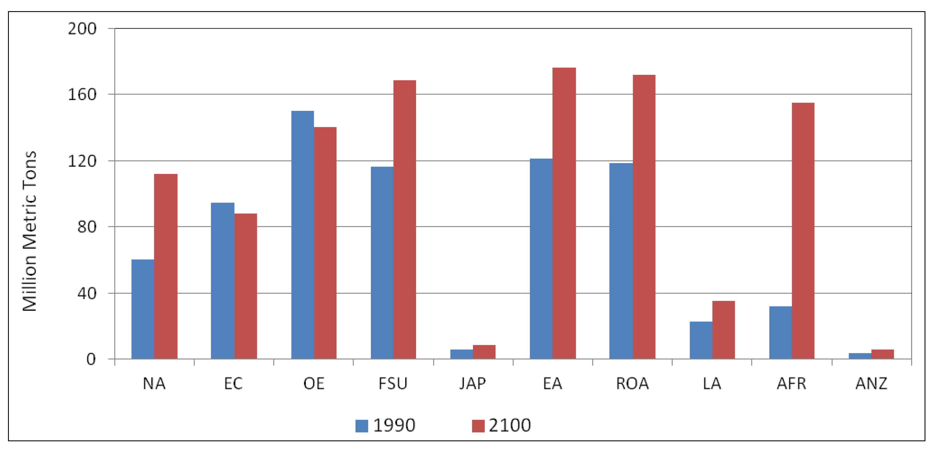
A feasible solution to the WTMCL for 2100 indicates that the projected regional demand for commodities can be satisfied. Our results show that in the absence of climate change, projected increases in demand due to population growth for the year 2100 do not jeopardize food availability: scenarios A1 and A2 are both feasible. When the effects of climate change are introduced, impacting the LGS under scenario B1, however, the scenario proves infeasible: in a world with climate change and without conversion of forestland to cropland, given the other scenario assumptions, the global agricultural system cannot produce enough output to satisfy global demand. Allowing for forestland conversions (scenario B2) delivers a feasible solution, as the forestland conversions compensate for the global average reduction in the productivity of lands associated with the climate change scenario.

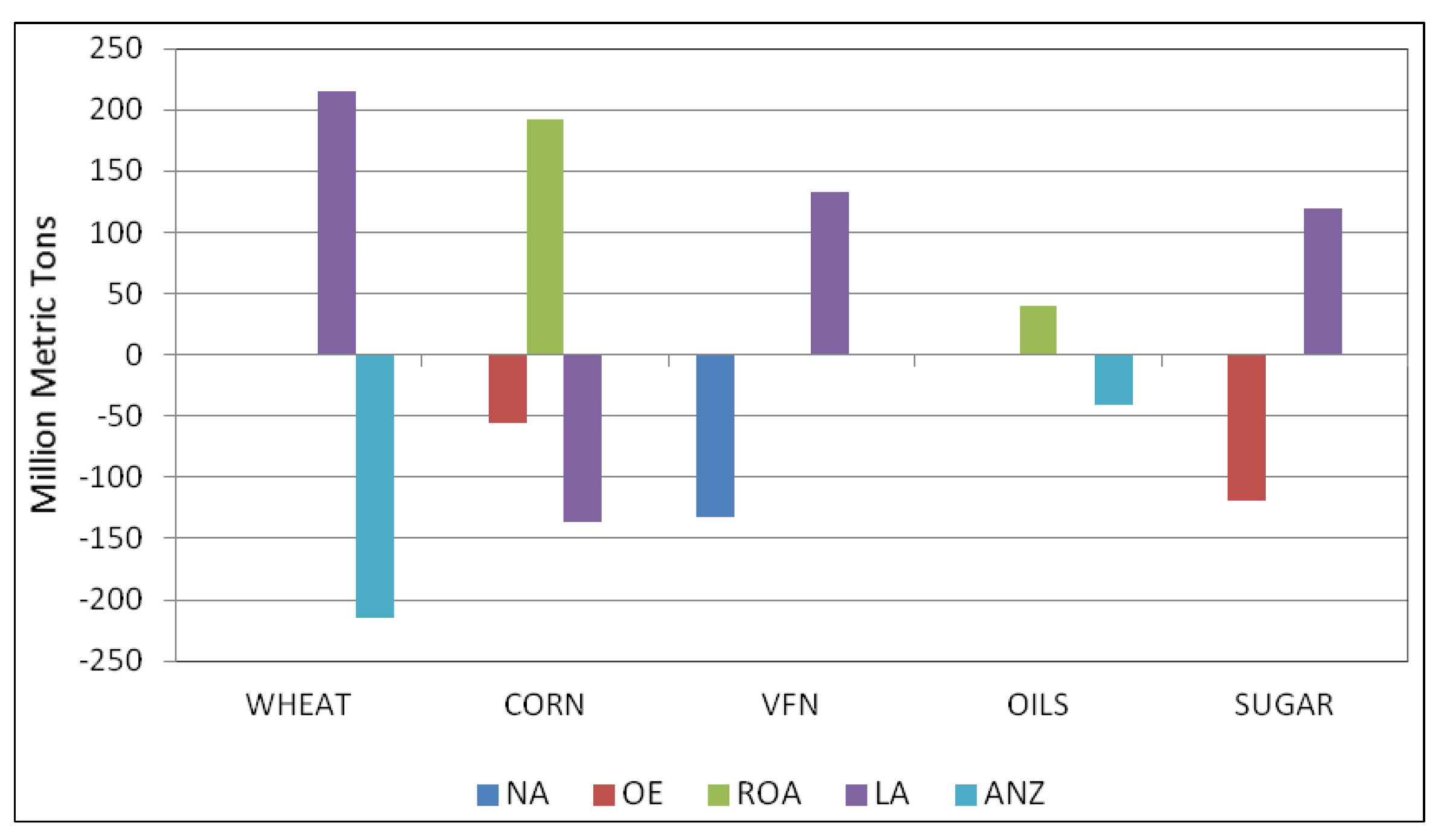
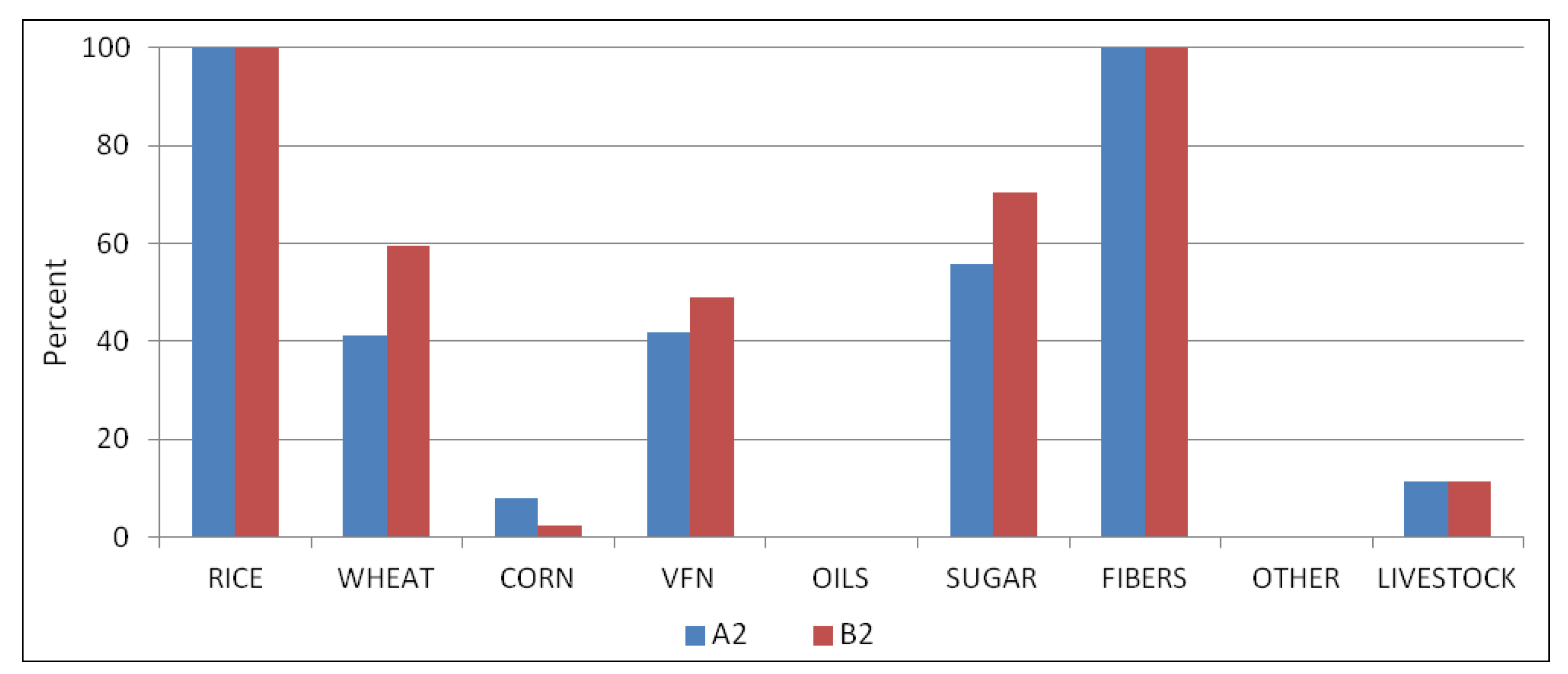
The outcome for B2 involves different patterns of regional specialization following changes in comparative advantage from its counterpart scenario without climate change, A2. Figure 4 illustrates some of the adjustments that take place: Latin America decreases production of corn, but increases the production of wheat, vegetables fruits and nuts, and sugar crops. Australia decreases the area devoted to wheat and oil crops, and North America the area devoted to vegetables, fruits and nuts. The Rest of Asia region gains comparative advantage for the production of corn and oil crops, while Other Europe loses comparative advantage for the production of both corn and sugar crops.

Figure 4. Regional change in the production of agricultural commodities from a scenario without climate change and forestland conversions (A2) to a scenario with climate change and forestland conversions (B2).

Figure 4. Regional change in the production of agricultural commodities from a scenario without climate change and forestland conversions (A2) to a scenario with climate change and forestland conversions (B2).

Note: See Section 2.1.3 for regional classification and commodity categories. Scenarios are described in Table 2. The figure shows only those agricultural commodities and regions for which the model solution reported changes.

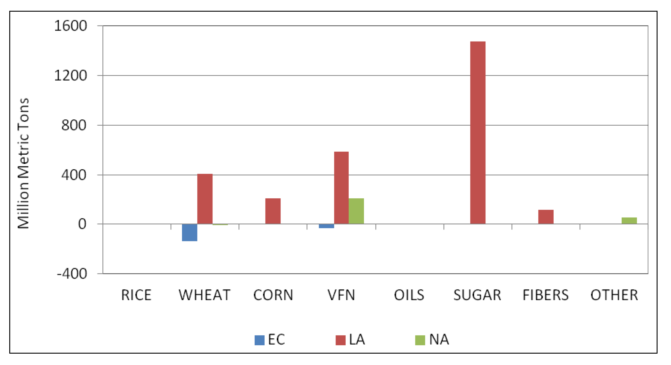
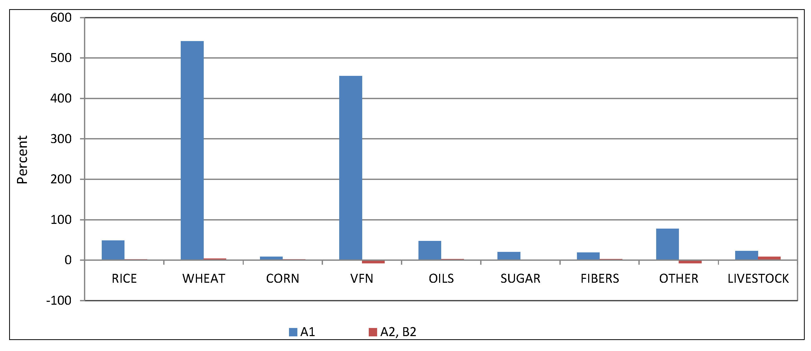
The differential impacts of forestland convertibility on comparative advantage in the absence of climate change are seen by comparing scenarios A1 and A2. In this case, differences are due to the relocation of production to regions where converted forestland had better productivity than the cropland replaced. Figure 5 illustrates some of these changes: The relatively high endowment of productive forestland allows Latin America to gain overwhelming cost advantages for the production of most crops due to the expansion onto the Amazon forests and the forested areas of the Brazilian Cerrado. However, the impacts on this region are even more pronounced under the climate change scenario B2. This is seen clearly in Figure 6.

Figure 5. Change in specialization from a scenario without forestland conversions (A1) to a scenario with forestland conversions (A2), both without the effects of climate change: selected regions.

Figure 5. Change in specialization from a scenario without forestland conversions (A1) to a scenario with forestland conversions (A2), both without the effects of climate change: selected regions.

Note: See Section 2.1.3 for regional classification and commodity categories. Scenarios are described in Table 2.

Figure 6. Percentage change in Latin America’s agricultural production, under a scenario without climate change and with forestland conversions (A2) and under a scenario with climate change and with forestland conversions (B2), both in relation to a scenario without climate change and without forestland conversions (A1).

Figure 6. Percentage change in Latin America’s agricultural production, under a scenario without climate change and with forestland conversions (A2) and under a scenario with climate change and with forestland conversions (B2), both in relation to a scenario without climate change and without forestland conversions (A1).

Note: See Section 2.1.3 for commodity categories. Scenarios are described in Table 2.

3.2. Land Use Change

Clearly, any loss of productivity of the world’s cropland as climate continues to change represents an obstacle to the achievement of global food security, and forestland conversions can compensate for such losses. In our simulations, climate change increases the amount of forestland conversions needed to satisfy the future global demand for food: under scenario A2 (without climate change), we find that 943 million hectares of forestland need to be converted while scenario B2 (with climate change) requires additional 20% of forests.

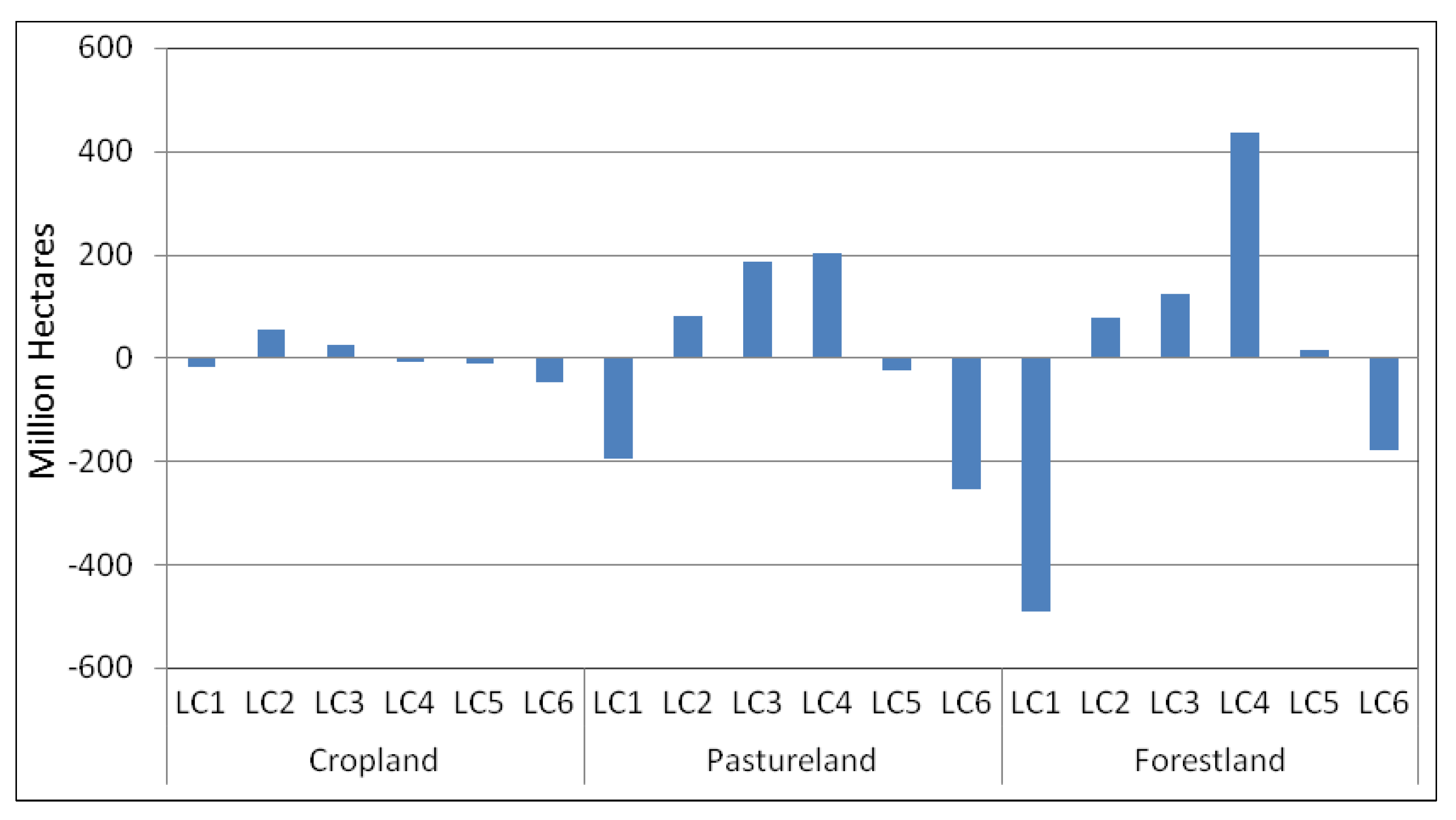
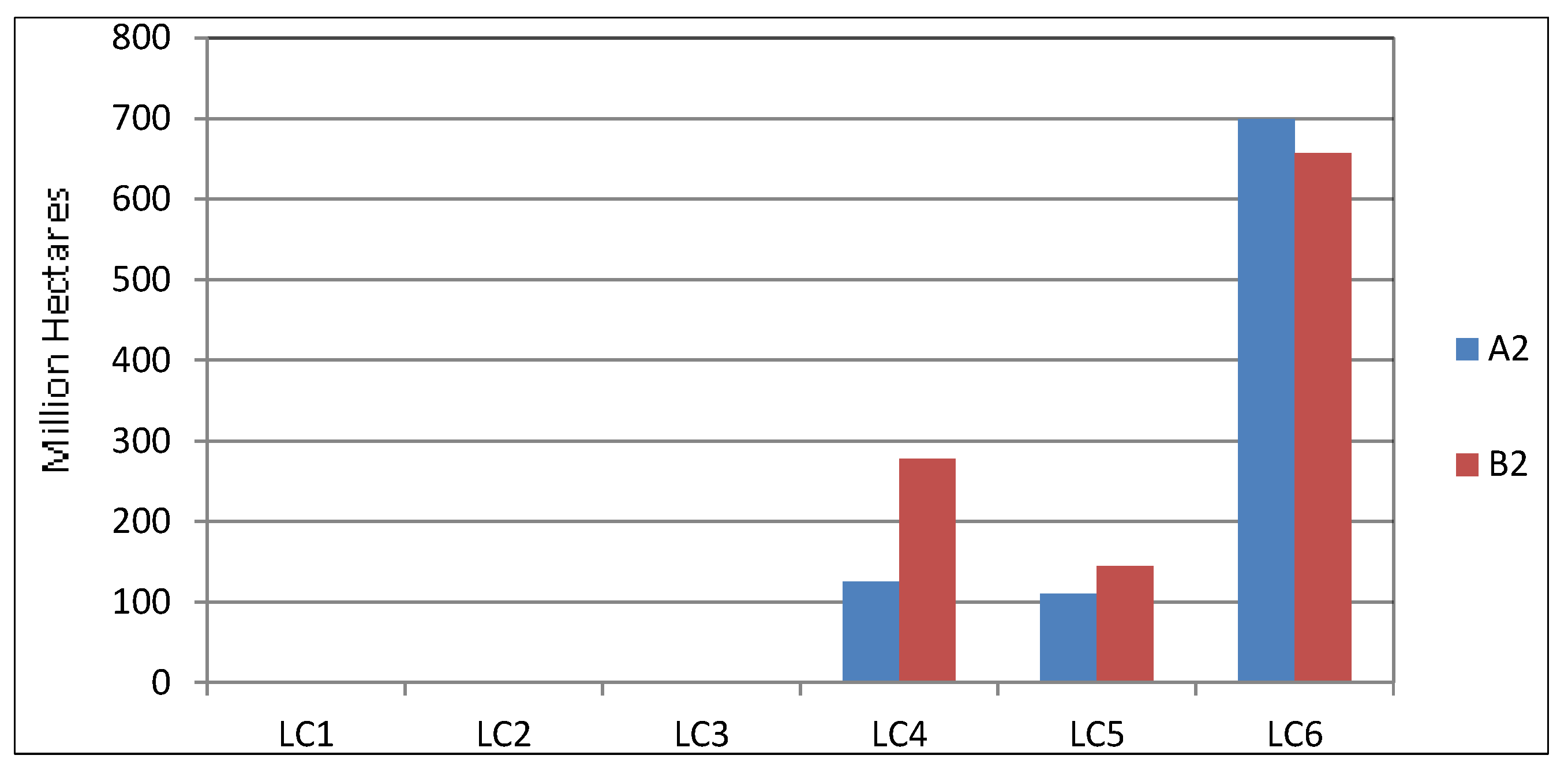
Almost all of the converted forestland under scenario B2 serves as cropland (less than one percent of the total is put to use as pastureland), and it is predominantly of types 4, 5 and 6 with the longest growing seasons. In fact, tropical land classes of type 6 account for over half the conversions (see Figure 7). Not surprisingly, Latin America, a region with forest endowments predominantly of type 5 and 6 available for clearing, show the highest rates of conversion, accounting for 75% or more of global figure (see Figure 8).

Figure 7. Global forestland conversions to cropland by land-class type under a scenario without climate change (A2) and under a scenario with climate change (B2).

Figure 7. Global forestland conversions to cropland by land-class type under a scenario without climate change (A2) and under a scenario with climate change (B2).

Note: Land classes (LC) are identified in Table 1. Scenarios are described in Table 2.

Figure 8. Regional forestland conversions to cropland by land-class type under a scenario without climate change (A2) and under a scenario with climate change (B2).

Figure 8. Regional forestland conversions to cropland by land-class type under a scenario without climate change (A2) and under a scenario with climate change (B2).

Note: See Section 2.1.3 for regional classification. Scenarios are described in Table 2.

The magnitudes and regional location of land conversions lie behind the changes in the regional allocation of production under alternative scenarios. An example of such shifts is provided by land-use changes in the European Community, which experiences reduced production of wheat and vegetables, fruits and nuts under scenario A2 (relative to scenario A1). Having relatively small endowments of land-class types 4, 5, and 6 available for conversion to cropland it loses its comparative advantage for the production of those crops to Latin America, a region that expands onto available forestland of types 5 and 6.

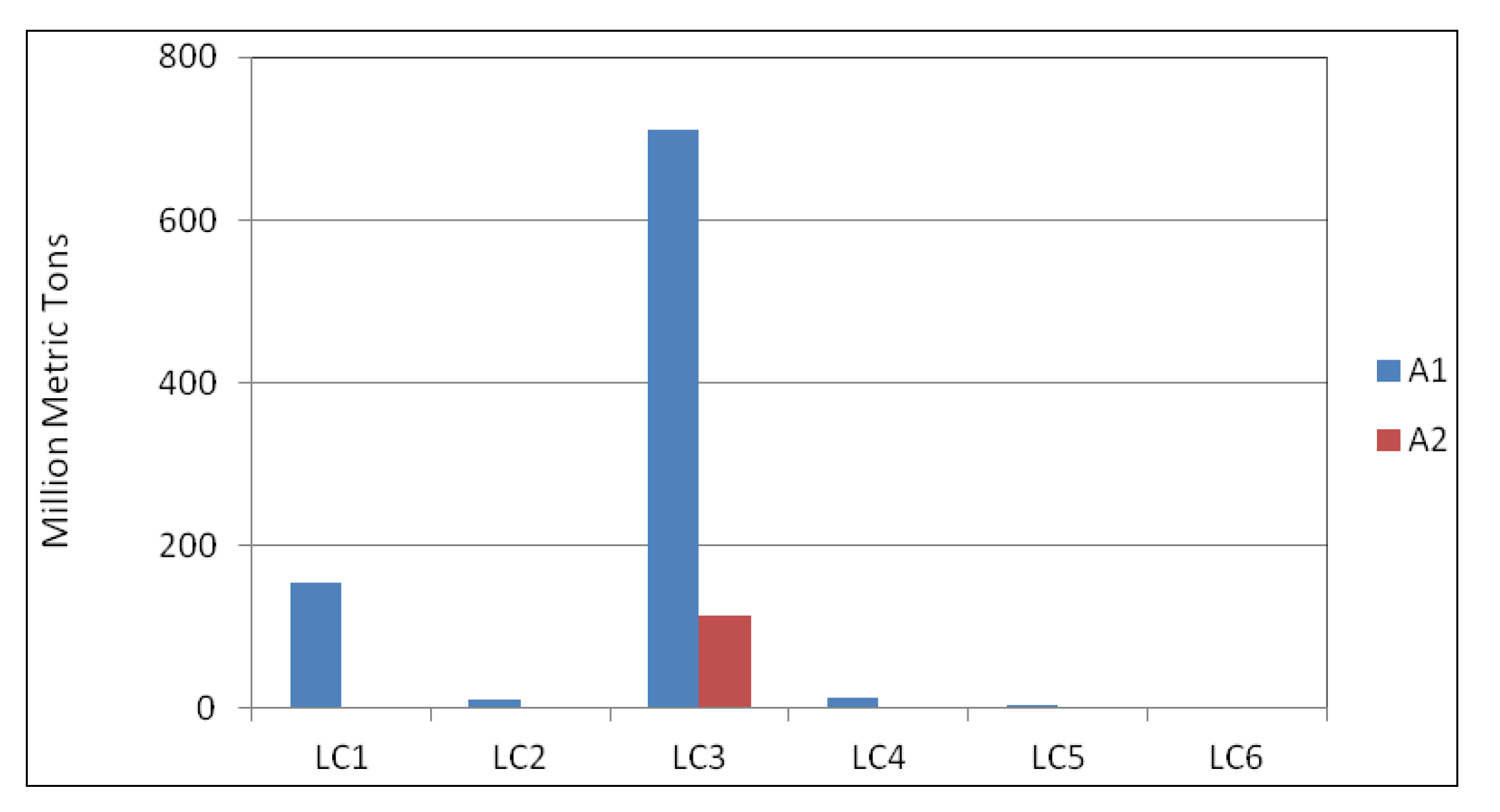
Changes in the patterns of land-class use and crop mix are also experienced within regions. Figure 9 illustrates the changes within the European Community in the allocation of land for the production of vegetables, fruits and nuts under scenarios A1 versus A2. Under scenario A2, which opens forestland for conversion in other regions (production partially moves to Latin America, see Figure 5), the production of this crop concentrates in the most suitable land-class, type 4, leaving the other land-class types uncultivated. Further comparison between scenarios A1 and A2 suggests that forestland conversion can be cost-saving when it allows production to expand onto land of higher productivity: the global cost of satisfying the same projected global demand (in the absence of climate change) is slightly lower (2%) under scenario A2 than under A1.

Figure 9. Land class type allocated for the production of vegetables, fruits and nuts in the European Community under two scenarios without climate change: one without forestland conversion (A1) and one with forestland conversion (A2).

Figure 9. Land class type allocated for the production of vegetables, fruits and nuts in the European Community under two scenarios without climate change: one without forestland conversion (A1) and one with forestland conversion (A2).

Note: Land classes (LC) are identified in Table 1. Scenarios are described in Table 2.

3.3. World Prices and Land Scarcity Rents

Prices of all agricultural commodities increase significantly from the benchmark scenario due to the effects of population growth, in the absence of both climate change and forestland conversions (i.e., under Scenario A1 relative to the 1990 baseline scenario). However, when forestland is converted to cropland under scenarios A2 and B2, price increases are very small; prices of a few crops even decrease slightly (see Figure 10). In our simulations, forestland conversion emerges as a powerful mechanism to mitigate agricultural price increases. In fact, allowing for forestland conversions in a world with climate change (the B2 scenario) results in world prices for agricultural commodities comparable to those in the absence of climate change (the A2 scenario). Such conversions compensate not only for regional shortages of cropland, as argued in the previous section, but also for any productivity losses associated with the new climatic conditions.

In the absence of forestland conversions, agricultural commodities must be produced in nearly all regions in order to satisfy the projected global food demand, and many of them (the ones with the relatively lowest costs of production) use their full endowment of cropland, which therefore earn positive scarcity rents. The dramatic increases in prices of wheat and of vegetables, fruits and nuts under scenario A1 (relative to the 1990 benchmark scenario) reflect large differences in costs among agricultural producers and the need for high-cost regions to produce and export. When high-cost regions produce, low-cost regions sell at the same price and earn scarcity rents that account for the difference between the world price and their (lower) costs. Table 4 shows an example. Under scenario A1 Australia and New Zealand (ANZ) devote all their land of land-class 4 to wheat, furnish a substantial share of global wheat production, and earn a large scarcity rent on this land. However, under scenario A2, other low-cost regions are able to expand their production of wheat. While this only slightly reduces the share of wheat produced in ANZ, the highest-cost producers under scenario A1 can no longer compete and fail to produce wheat. This brings down the world price, to the extent that ANZ now devotes less than a third of its land-class 4 land to wheat and fails to earn a scarcity rent on it. The substantial change in the price of wheat is shown in Figure 10.

Table 4. Land use for the production of wheat and scarcity rents reported by land-class category in Australia and New Zealand.

	Scenario A1			Scenario A2
	Land Use for Wheat (% of endowment)	Scarcity Rent (1990 U$/ha)	Production (% of global)	Land Use (% of endowment)	Scarcity Rent (1990 U$/ha)	Production (% of global)
LC1	0.0	0.0	0.0	0.0	0.0	0.0
LC2	0.0	0.0	0.0	0.0	0.0	0.0
LC3	0.0	0.0	0.0	0.0	0.0	0.0
LC4	100	16.2	62.9	29	0.0	58.7
LC5	0.0	0.0	0.0	0.0	0.0	0.0
LC6	0.0	0.0	0.0	0.0	0.0	0.0

Note: Land classes (LC) are identified in Table 1. Scenarios A1 and A2 are described in Table 2.

Table 4. Land use for the production of wheat and scarcity rents reported by land-class category in Australia and New Zealand.

	Scenario A1			Scenario A2
	Land Use for Wheat (% of endowment)	Scarcity Rent (1990 U$/ha)	Production (% of global)	Land Use (% of endowment)	Scarcity Rent (1990 U$/ha)	Production (% of global)
LC1	0.0	0.0	0.0	0.0	0.0	0.0
LC2	0.0	0.0	0.0	0.0	0.0	0.0
LC3	0.0	0.0	0.0	0.0	0.0	0.0
LC4	100	16.2	62.9	29	0.0	58.7
LC5	0.0	0.0	0.0	0.0	0.0	0.0
LC6	0.0	0.0	0.0	0.0	0.0	0.0

Note: Land classes (LC) are identified in Table 1. Scenarios A1 and A2 are described in Table 2.

Figure 10. Percentage change in world prices of agricultural commodities, from the 1990 benchmark scenario to a scenario without climate change and without forestland conversions (A1) and to scenarios with forestland conversion, one without climate change (A2) and one with climate change (B2).

Figure 10. Percentage change in world prices of agricultural commodities, from the 1990 benchmark scenario to a scenario without climate change and without forestland conversions (A1) and to scenarios with forestland conversion, one without climate change (A2) and one with climate change (B2).

Note: See Section 2.1.3 for commodity categories. Scenarios are described in Table 2.

4. Conclusions and Discussion

This paper presents a modeling framework, the World Trade Model with Climate Sensitive Land [1], for anticipating land-use change that may take place in response to climate change and increased demand for agricultural commodities. The approach differs from most economic approaches used to model changes in land use in that rather than assigning exogenous values to Armington trade elasticities and elasticities of transformation to regulate the ease with which regions rely on specific tarde partners (or any partners) and the ease with which land can be converted to alternative uses. Our approach allows regional agricultural production to follow comparative advantage and in the process determines patterns of land use in all regions of the world. The study evaluates four scenarios that combine assumptions about increases in food demand with changes in climatic conditions and convertibility of forestland to agricultural land. The analysis investigates the likely state of food availability under the simulated conditions, the magnitude and directional change in land use that adaptations to climate change may generate, and the directional change in future prices of the major agricultural commodity groups.

Results suggest that satisfying projected future global agricultural demand will make it difficult to preserve today’s forestland areas intact in the presence of anticipated climatic change. Climate change is likely to increase the extent of cropland required to satisfy any given volume of food demand, and scarcity of the world’s cropland emerges as the limiting factor to future food availability. Allowing for forestland conversions, however, makes it possible to satisfy future agricultural requirements under the projected changes in climate. Forestland conversion to cropland, and to a lesser extent to pastureland, can in principle compensate for the reduced yields associated with climate change and with increases in demand. Adjustments mechanisms entail regional changes in the mix of agricultural products and in the area devoted to agriculture.

In our simulations, conversion of about 25% of current forestland is required, with Latin America exhibiting the highest degree of deforestation. Forestland conversion to cropland emerges as a tempting option to overcome the pressure that population growth and climate change may impose on future generations. This finding is of great concern, given the vital ecosystem services provided by forests, in particular tropical forests like the Amazon rainforest and the wooded savannah of the Brazilian Cerrado, as carbon sinks and as stabilizers of the global climate. A central challenge for global sustainability becomes then how to preserve forest ecosystems and the services they provide while enhancing food production. This challenge cannot be avoided, as the forces of environmental change and economic globalization are combining in ways that trigger deforestation of huge tracts of land [8].

Our results suggest that economic motives for deforestation are likely to be extremely strong not only due to potential future shortages of food created by the shrinking availability of cropland, but also because relocating global production to climatically-suitable converted forestland offers only small increases—and even decreases—in world food prices relative to benchmark prices. When forestland conversion is not allowed, agricultural prices increase steeply: the price of wheat, for example, rises to about four times the benchmark price. In this case, shortages of available agricultural land, especially cropland, bring increased rents associated with their scarcity to the owners of the most productive lands and other scarce inputs. The price of wheat, however, falls to only about 10% above the benchmark price when deforestation is permitted, providing a strong economic incentive for further clearing. Incentives could be compounded by net losses in productivity of agricultural land areas due to factors such as erosion, as well as by competing claims on land for alternative uses such as the production of crops for biofuels.

The substantial rates of deforestation according to our scenario outcomes may be avoided by policy interventions and management practices. Two common strategies proposed to control deforestation and expansion of agriculture into forested and fragile ecosystems are land-use zoning and agricultural intensification, the latter as a way to spare land for nature as higher yields decrease the extent of land required. Adaptations to climate change that involve increased reliance on international trade as discussed in this article, however, may render the above strategies less effective in controlling land uses, especially efforts to maintain tropical forests [8]. At the same time, international trade also has the potential to increase global land-use efficiency by allowing for regional specialization in areas of comparative advantage [10]. Global adaptations to climate change of the sort captured by the WTMCL framework, which re-allocate production to the most suitable land areas, may be harnessed to increase land-use efficiency rather than leading to uncontrolled land-use expansion.

Land-use changes are cumulatively a major driver of global environmental change [16]. Designing policies to reconcile land-use development paths with the preservation of vital ecosystems and the services they provide requires understanding land-use change as part of global scale, open systems [8]. The methodological approach and results of the study described in this article increase the diversity of case studies and approaches that improve understanding of the challenges and opportunities for preserving natural forest ecosystems while enhancing food production under conditions of global cropland scarcity and environmental change.

Simplifying assumptions made throughout the analysis can be relaxed in further research. Improving agricultural productivity and shifting toward less resource-intensive diets are additional mechanisms for dealing with climate change under conditions of scarcity of productive cropland [17]. The solutions to our scenarios exhibit a higher degree of regional specialization than what is actually observed; next steps could evaluate the impacts of protectionist trade policies or the imposition of other constraints, the most obvious one being water scarcity. We and our colleagues incorporate water as a factor of production in companion studies that include scenarios about the restriction of water withdrawals, including through caps or pricing [17,18,19,20]. Additional scenarios to consider in this context involve the analysis of policies to promote increased regional self-reliance on food.

References

1. Juliá, R.; Duchin, F. World trade as the adjustment mechanism of agriculture to climate change. Clim. Chang. 2007, 82, 393–409. [Google Scholar] [CrossRef]
2. Parry, M.L.; Rosenzweig, C.; Iglesias, A.; Livermore, M.; Fischer, G. Effects of climate change on global food production under SRES emissions and socio-economic scenarios. Global Environ. Change 2004, 14, 53–67. [Google Scholar] [CrossRef]
3. Randhir, T.; Hertel, T.W. Trade liberalization as a vehicle for adapting to global warming. Agric. Resour. Econ. Rev. 2000, 29, 1–14. [Google Scholar]
4. Reilly, J.; Hohmann, N.; Kane, S. Climate change and agricultural trade: Who benefits, who loses. Global Environ. Change 1994, 4, 24–36. [Google Scholar] [CrossRef]
5. Rosenzweig, C.; Parry, M.L. Potential impacts of climate change on world food supply. Nature 1994, 367, 133–139. [Google Scholar] [CrossRef]
6. Long, S.P.; Ainsworth, E.A.; Leakey, A.D.B.; Nösberger, J.; Ort, D.R. Food for thought: Lower-than-expected crop yield stimulation with rising CO2 concentrations. Science 2006, 312, 1918–1921. [Google Scholar] [CrossRef]
7. Tubiello, F.N.; Fischer, G. Reducing climate change impacts on agriculture: Global and regional effects of mitigation, 2000–2080. Technol. Forecast. Soc. Change 2007, 74, 1030–1056. [Google Scholar] [CrossRef]
8. Lambin, E.F.; Meyfroidt, P. Global land use change, economic globalization, and the looming land scarcity. Proc. Natl. Acad. Sci. USA 2011, 108, 3465–3472. [Google Scholar] [CrossRef]
9. Gibbs, H.K.; Ruesch, A.S.; Achard, M.K.; Clayton, M.K.; Holmgren, P.; Ramankutty, N.; Foley, A. Tropical forests were the primary sources of new agricultural land in the 1980s and 1990s. Proc. Natl. Acad. Sci. USA 2010, 107, 16732–16737. [Google Scholar] [CrossRef]
10. Meyfroidt, P.; Rudel, T.K.; Lambin, E.F. Forest transitions, trade, and the global displacement of land use. Proc. Natl. Acad. Sci. USA 2010, 107, 20917–20922. [Google Scholar] [CrossRef]
11. Khanna, M.; Crago, C. Measuring indirect land use change with biofuels: Implications for policy. Annu. Rev. Resour. Econ. 2012, 4, 161–184. [Google Scholar] [CrossRef]
12. Duchin, F. A world trade model based on comparative advantage with m regions, n goods and k factors. Econ. Syst. Res. 2005, 17, 141–162. [Google Scholar] [CrossRef]
13. Darwin, R.F.; Tsigas, M.; Lewandrowski, J.; Raneses, A. World Agriculture and Climate Change: Economic Adaptations. U.S. Department of Agriculture, Agricultural Economic Research Service, Economic Report No. 703; 1995. Available online: http://www.ers.usda.gov (accessed on 9 September 2013). [Google Scholar]
14. Duchin, F.; Levine, S.H. Sectors may use multiple technologies simultaneously: The rectangular choice-of-technology model with binding factor constraints. Econ. Syst. Res. 2011, 23, 281–302. [Google Scholar] [CrossRef]
15. Hansen, J.; Fung, I.; Lacis, A.; Rind, D.; Lebedeff, S.; Ruedy, R.; Russell, G. Global climate change as forecasted by the goddard institute for space studies three-dimensional model. J. Geophys. Res. 1988, 93, 9341–9364. [Google Scholar] [CrossRef]
16. Turner, B.L.; Lambin, E.F.; Reenberg, A. The emergence of land change science for global environmental change and sustainability. Proc. Natl. Acad. Sci. USA 2007, 104, 20666–20671. [Google Scholar] [CrossRef]
17. Springer, N.; Duchin, F. Feeding nine billion people sustainably: Conserving land and water through shifting diets and changes in technologies. Environ. Sci. Technol. 2013. submitted for publication. [Google Scholar]
18. López-Morales, C.; Duchin, F. Policies and technologies for a sustainable use of water in Mexico: A scenario analysis. Econ. Syst. Res. 2011, 23, 387–407. [Google Scholar] [CrossRef]
19. Duchin, F.; López-Morales, C. Do water-rich regions have a comparative advantage in food production? Improving the representation of water for agriculture in economic models. Econ. Syst. Res. 2012, 24, 371–389. [Google Scholar] [CrossRef]
20. López-Morales, C.; Duchin, F. Achieving water sustainability: Analyzing scenarios restricting water withdrawals from surface and underground sources with an inter-regional model of the mexican economy. Environ. Sci. Technol. 2013. submitted for publication. [Google Scholar]
Appendix
The World Trade Model with Climate Sensitive Land (WTMCL).
Primal Problem:
Sustainability 05 05442 i001
Sustainability 05 05442 i002
Sustainability 05 05442 i003
Sustainability 05 05442 i004
Sustainability 05 05442 i005
Dual Problem:
Sustainability 05 05442 i006