General Spatiotemporal Patterns of Urbanization: An Examination of 16 World Cities

Abstract

Urbanization is the most dramatic form of land use change that has profoundly influenced environmental and socioeconomic conditions around the world. To assess these impacts and promote urban sustainability, a better understanding of urbanization patterns is needed. Recent studies have suggested several spatiotemporal patterns of urbanization, but their generality is yet to be adequately tested with long-term data. Thus, the main goal of our study was two-fold: (1) to examine the spatiotemporal patterns of urbanization of 16 world cities over a period of 200 years (1800–2000); and (2) to test four prominent hypotheses of urbanization patterns. Using a set of landscape metrics, we quantified temporal changes in the urban landscape pattern of the 16 cities and examined the four hypotheses individually. Our results show that these cities exhibit several common urbanization patterns: the urban landscape becomes compositionally more diverse, structurally more fragmented and geometrically more complex as urbanization progresses. Our study also suggests that urbanization is a process of shifting dominance among three urban growth modes: infilling, edge expanding and leapfrogging. However, idiosyncrasies do exist for individual cities, as detailed attributes of urbanization patterns often depend on the environmental and socioeconomic settings of cities. In addition, the choice of specific landscape metrics and the scales of analysis both influence the urbanization patterns revealed. Our study examined the urbanization patterns, for the first time, on long-term and global scales. The findings shed new light on the patterns and processes of urbanization, with implications for future studies of the ecology, planning and sustainability of cities.

1. Introduction

Urbanization across the world has resulted in dramatic changes in landscape patterns and profound effects on biodiversity, ecological processes and regional sustainability [1,2,3,4,5,6]. From 2010–2050, the percentage of the global urban population is projected to increase from 51.6%–67.2% [7], while the global built-up area will increase three times [8]. To assess the impacts of urbanization on ecosystems and regional sustainability, understanding the spatiotemporal patterns of urbanization is an important and necessary step [9,10].

The importance of understanding urbanization patterns is evidenced by the increasing number of studies around the world during the past few decades [5,6,11,12,13,14,15,16,17]. For example, Dietzel et al. analyzed the spatiotemporal dynamics of the built-up area in the Central Valley of California from 1940–2040 and in the Houston Metropolitan Area from 1974–2002, concluding that urbanization is a two-step alternating process of diffusion and coalescence [18,19]. Li et al. quantified the spatiotemporal patterns of urbanization in the central Yangtze River Delta region, China, from 1979–2008, describing urbanization “as a spiraling process of shifting dominance among three urban growth modes: the wax and wane of infilling, edge-expansion, and leapfrog” [20]. Based on their long-term ecological research in the Phoenix metropolitan region, Wu et al. stated that “the general pattern of urbanization was that the increasingly urbanized landscape became compositionally more diverse, geometrically more complex, and ecologically more fragmented” [10,21,22,23]. Since 2000, numerous studies have reported similar findings concerning urbanization patterns [24,25,26].

These findings have provided much insight into urbanization patterns and their underlying processes, showing both common and idiosyncratic features among cities, which depend on city size, socioeconomic drivers, land use policies and the scale of analysis. However, a comprehensive examination of these findings with cities in different parts of the world is lacking. It remains unclear, therefore, whether these observed patterns of urbanization are general and whether they change with scales in time and space. To address these questions requires comparing and contrasting a number of cities together, using consistent methods and long-term data (at least several decades or longer). Such studies have been hindered by the lack of data and other related logistical reasons.

Figure 1. Changes in landscape metrics measuring urbanization patterns on the basis of three hypotheses. (a1–a6) Based on the “diffusion and coalescence” hypothesis [18,19]; (b1–b3) based on the “diversity-complexity” hypothesis [10,21,22,23]; (c1–c4) based on the “landscape modification gradient” hypothesis [27]. The X axis denotes the process of urbanization; the Y axis denotes the value of landscape metrics measuring urbanization patterns. Landscape metrics include: patch density (PD), edge density (ED), mean Euclidean nearest neighbor distance (NND), area-weighted mean fractal dimension (AWMFD), mean patch size (MPS), contagion, the landscape shape index (LSI) and Shannon’s diversity index (SHDI) (see Table 2 for details).

Figure 1. Changes in landscape metrics measuring urbanization patterns on the basis of three hypotheses. (a1–a6) Based on the “diffusion and coalescence” hypothesis [18,19]; (b1–b3) based on the “diversity-complexity” hypothesis [10,21,22,23]; (c1–c4) based on the “landscape modification gradient” hypothesis [27]. The X axis denotes the process of urbanization; the Y axis denotes the value of landscape metrics measuring urbanization patterns. Landscape metrics include: patch density (PD), edge density (ED), mean Euclidean nearest neighbor distance (NND), area-weighted mean fractal dimension (AWMFD), mean patch size (MPS), contagion, the landscape shape index (LSI) and Shannon’s diversity index (SHDI) (see Table 2 for details).

In this study, we took advantage of the recently available long-term data of global urbanization (see the Materials and Methods for detail) and attempted to address the questions of generality and idiosyncrasy in urbanization patterns. Specifically, our main objectives are two-fold: (1) to identify the generalities and idiosyncrasies in the spatiotemporal patterns of the urbanization of the world’s major cities over a period of 200 years (1800–2000); and (2) to test several hypotheses of urbanization patterns. These hypotheses include:

(1)

the “diffusion and coalescence” hypothesis, which describes urbanization as an alternative process of diffusion and coalescence (Figure 1a) [18,19];

(2)

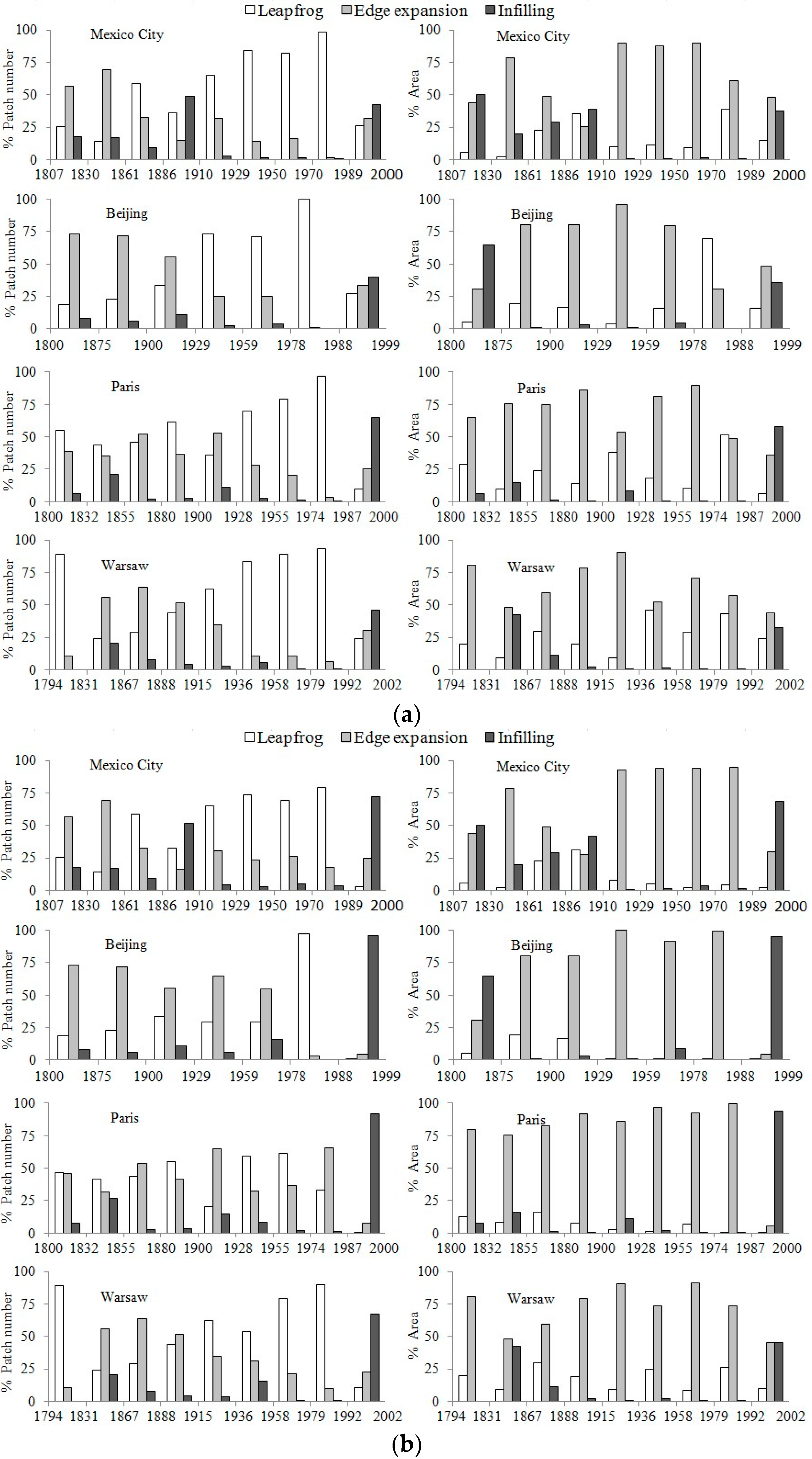
the three growth mode hypothesis, which characterizes urbanization as a wax and wane process of infilling, edge expansion and leapfrogging [20];

(3)

the “landscape modification gradient” hypothesis, which states that, with increasing human modification to the landscape from natural to urban, patch density and shape regularity increase, whereas mean patch size and landscape connectivity decrease (Figure 1c) [27]; and

(4)

the diversity-complexity hypothesis that urbanization results in landscape patterns with increasing compositional diversity, geospatial complexity and ecological fragmentation (Figure 1b) [10,21,22,23].

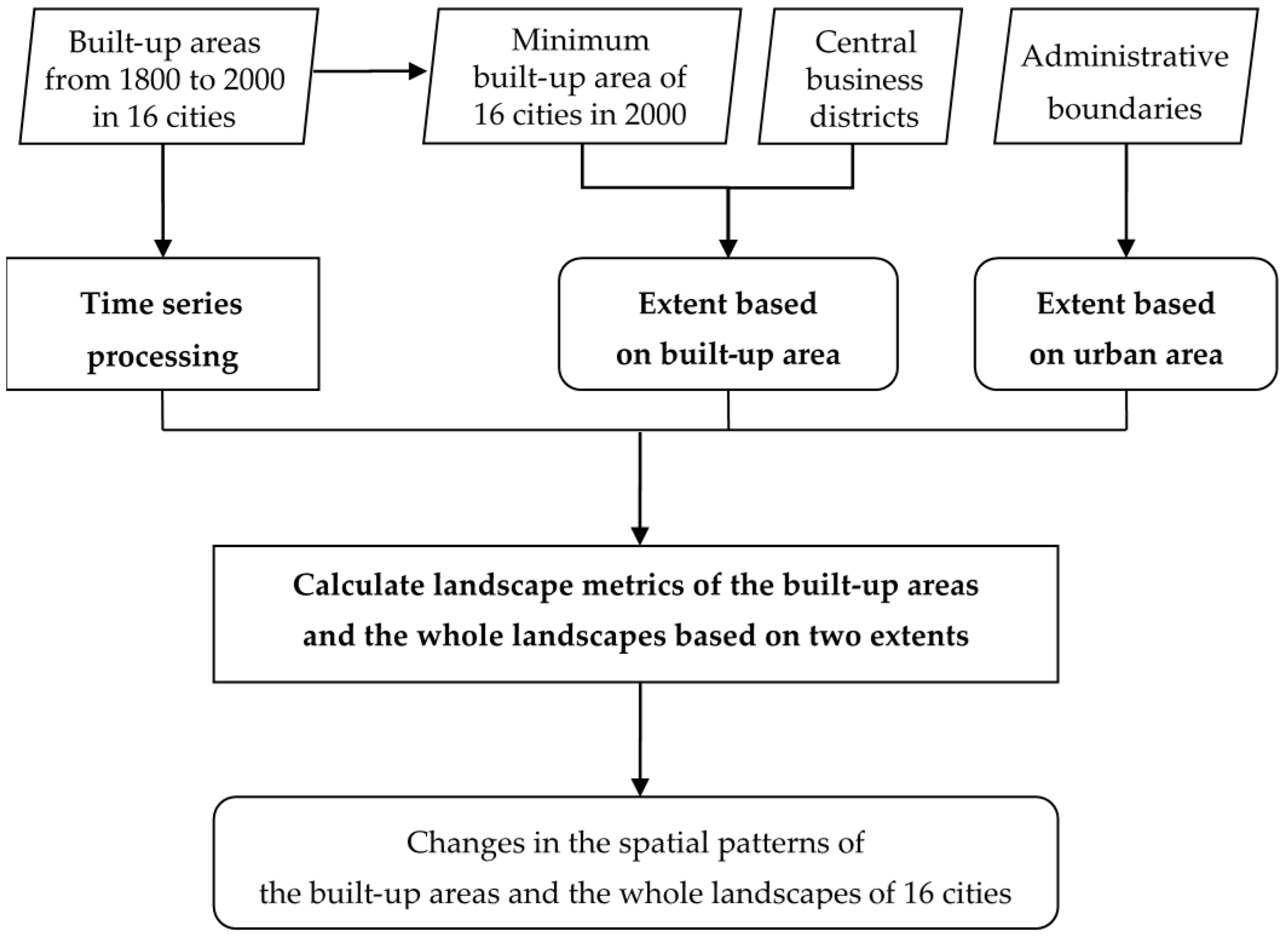
2. Materials and Methods

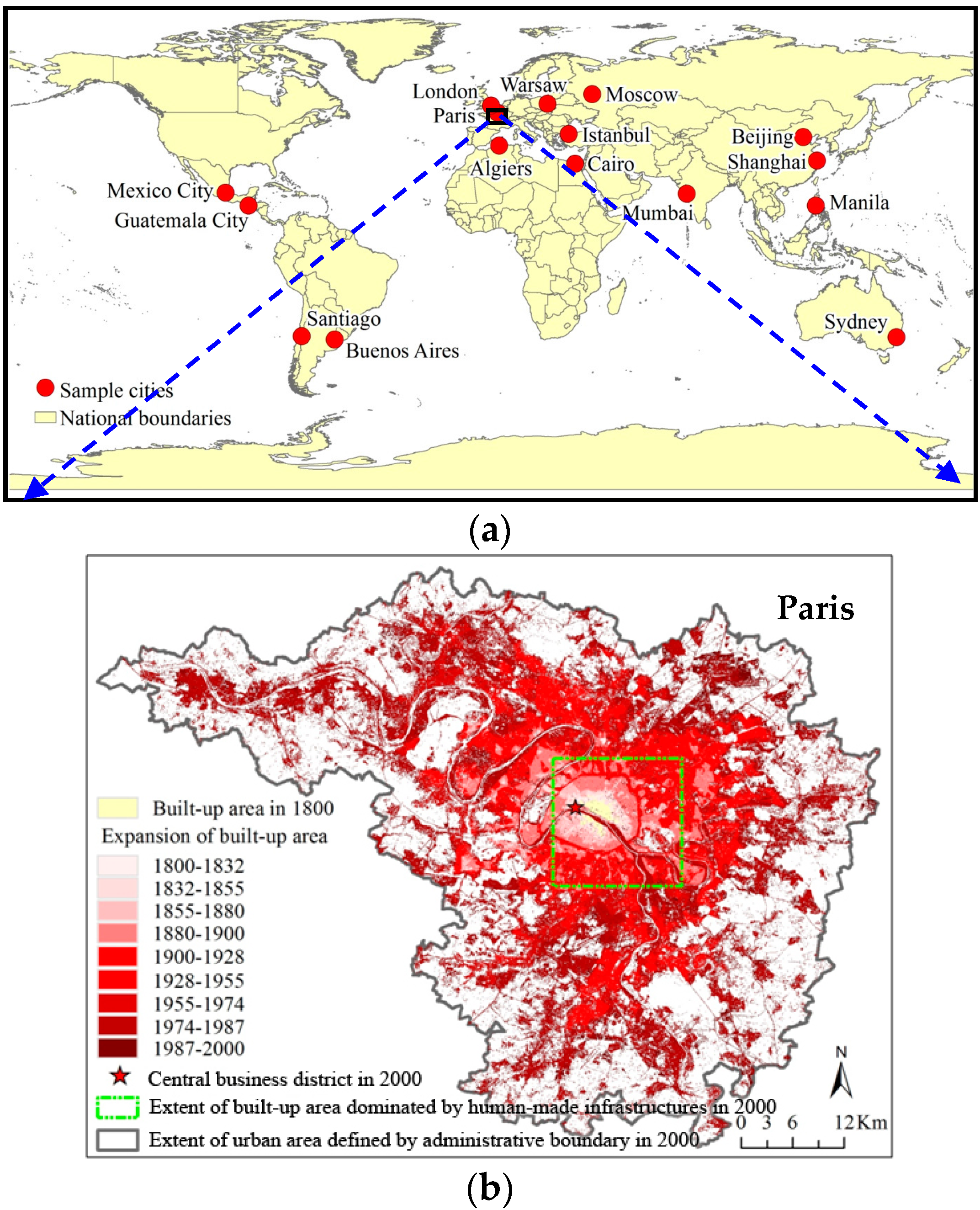
2.1. Data Acquisition and Processing

The primary data source for our study was the Dataset of the Global Historical Sample of 30 Cities in the Atlas of Urban Expansion, produced by the Lincoln Institute of Land Policy [24] (available at the institute’s website) (Table 1, Figure 2) [28]. Among the 30 sample cities, we chose 16 major cities around the world whose data on built-up areas from 1800–2000 were most complete, including Algiers, Beijing, Buenos Aires, Cairo, Guatemala City, Istanbul, London, Manila, Mexico City, Moscow, Mumbai, Paris, Santiago, Shanghai, Sydney and Warsaw (Table 1). To produce the built-up areas over the 200-year period, both remote sensing imageries and historical maps were used [29]. For the period of 1990–2000, the built-up areas were extracted from two Landsat satellite images at a resolution of 28.5 m, one as close as possible to 1990 and one as close as possible to 2000. The extracted built-up areas were further validated using high-resolution remote sensing data in Google Earth, with a producer accuracy of 91% and a user accuracy of 89% [29]. Before 1990, the built-up areas were interpreted from historical maps (Supplementary S1). These historical maps were first geo-referenced and then converted to digital formats. After that, the built-up areas in these maps were digitized to vector files. Besides the built-up areas, the administrative boundaries in 2000, the locations of central business districts (CBD) in 2000 and the urban population from 1800–2000 of 16 cities were also obtained from the Atlas of Urban Expansion (Figure 2b).

Table 1. List of the 16 study cities.

World Region *	Host Country	City	Urban Population in 2000 (millions)	Years with Data on Built-up Area **
South-Eastern Asia	Philippines	Manila	17.34	1802, 1831, 1842, 1884, 1898, 1918, 1945, 1971, 1993, 2002
South-Central Asia	India	Mumbai	16.16	1814, 1849, 1865, 1888, 1909, 1931, 1955, 1968, 1992, 2001
Eastern Asia	China	Shanghai	14.13	1810, 1853, 1875, 1902, 1914, 1944, 1973, 1989, 2001
	China	Beijing	11.87	1800, 1875, 1900, 1929, 1959, 1978, 1988, 1999
Western Asia	Turkey	Istanbul	8.83	1807, 1840, 1872, 1899, 1916, 1934, 1960, 1987, 2000
Central America	Mexico	Mexico City	17.22	1807, 1830, 1861, 1886, 1910, 1929, 1950, 1970, 1989, 2000
	Guatemala	Guatemala City	1.77	1800, 1850, 1900, 1936, 1950, 1976, 1993, 2000
South America	Argentina	Buenos Aires	11.92	1809, 1836, 1867, 1887, 1918, 1943, 1964, 1987, 2000
	Chile	Santiago	5.34	1800, 1850, 1875, 1900, 1930, 1950, 1970, 1989, 2000
Northern Europe	United Kingdom	London	10.03	1800, 1830, 1860, 1880, 1914, 1929, 1955, 1978, 1989, 2000
Western Europe	France	Paris	9.52	1800, 1832, 1855, 1880, 1900, 1928, 1955, 1974, 1987, 2000
Eastern Europe	Russia	Moscow	9.14	1808, 1836, 1893, 1914, 1939, 1957, 1978, 1991, 2002
	Poland	Warsaw	2.00	1794, 1831, 1867, 1888, 1915, 1936, 1958, 1979, 1992, 2002
Northern Africa	Egypt	Cairo	13.08	1800, 1846, 1874, 1897, 1917, 1927, 1947, 1960, 1984, 2000
	Algeria	Algiers	3.63	1800, 1828, 1858, 1888, 1903, 1929, 1955, 1972, 1987, 2000
Oceania	Australia	Sydney	4.23	1808, 1833, 1860, 1883, 1895, 1917, 1945, 1975, 1993, 2002

* Please refer to the World Urbanization Prospects from the United Nations for the details of world region classification (http://esa.un.org/unpd/wup/); ** please refer to Supplementary S1 for the details of the data source.

Table 1. List of the 16 study cities.

World Region *	Host Country	City	Urban Population in 2000 (millions)	Years with Data on Built-up Area **
South-Eastern Asia	Philippines	Manila	17.34	1802, 1831, 1842, 1884, 1898, 1918, 1945, 1971, 1993, 2002
South-Central Asia	India	Mumbai	16.16	1814, 1849, 1865, 1888, 1909, 1931, 1955, 1968, 1992, 2001
Eastern Asia	China	Shanghai	14.13	1810, 1853, 1875, 1902, 1914, 1944, 1973, 1989, 2001
	China	Beijing	11.87	1800, 1875, 1900, 1929, 1959, 1978, 1988, 1999
Western Asia	Turkey	Istanbul	8.83	1807, 1840, 1872, 1899, 1916, 1934, 1960, 1987, 2000
Central America	Mexico	Mexico City	17.22	1807, 1830, 1861, 1886, 1910, 1929, 1950, 1970, 1989, 2000
	Guatemala	Guatemala City	1.77	1800, 1850, 1900, 1936, 1950, 1976, 1993, 2000
South America	Argentina	Buenos Aires	11.92	1809, 1836, 1867, 1887, 1918, 1943, 1964, 1987, 2000
	Chile	Santiago	5.34	1800, 1850, 1875, 1900, 1930, 1950, 1970, 1989, 2000
Northern Europe	United Kingdom	London	10.03	1800, 1830, 1860, 1880, 1914, 1929, 1955, 1978, 1989, 2000
Western Europe	France	Paris	9.52	1800, 1832, 1855, 1880, 1900, 1928, 1955, 1974, 1987, 2000
Eastern Europe	Russia	Moscow	9.14	1808, 1836, 1893, 1914, 1939, 1957, 1978, 1991, 2002
	Poland	Warsaw	2.00	1794, 1831, 1867, 1888, 1915, 1936, 1958, 1979, 1992, 2002
Northern Africa	Egypt	Cairo	13.08	1800, 1846, 1874, 1897, 1917, 1927, 1947, 1960, 1984, 2000
	Algeria	Algiers	3.63	1800, 1828, 1858, 1888, 1903, 1929, 1955, 1972, 1987, 2000
Oceania	Australia	Sydney	4.23	1808, 1833, 1860, 1883, 1895, 1917, 1945, 1975, 1993, 2002

* Please refer to the World Urbanization Prospects from the United Nations for the details of world region classification (http://esa.un.org/unpd/wup/); ** please refer to Supplementary S1 for the details of the data source.

Figure 2. The locations of the 16 study cities (a) and, as an example, the urbanization map of Paris, illustrating urban expansion from 1800–2000 (b) (see Table 1 for details).

Figure 2. The locations of the 16 study cities (a) and, as an example, the urbanization map of Paris, illustrating urban expansion from 1800–2000 (b) (see Table 1 for details).

After the data acquisition, all of the vector files of historical built-up areas were converted to raster data at a resolution of 28.5 m to be consistent with the data from 1990–2000. Then, we performed a time series correction to improve the continuity and comparability of the built-up areas in different years (Figure 3). According to Angel et al. [8], built-up areas could be assumed to continuously increase from 1800–2000, and a pixel of the built-up area detected in an earlier year would remain as built-up area in a later year. Based on this assumption, we implemented the time series correction as summarized by the following formula:

$$D{N}_{(n,i)}=\{\begin{array}{cc}0& D{N}_{(n+1,i)}=0\\ D{N}_{(n,i)}& otherwise\end{array}$$

(1)

where $D{N}_{(n,i)}$ and $D{N}_{(n+1,i)}$ are the class values (built-up area or not) at the i-th pixel in the n-th and n + 1th years, respectively. A class value of 1 represents built-up area, while 0 represents non-built-up area.

Figure 3. A flowchart of the key steps in data acquisition, processing and analysis.

Figure 3. A flowchart of the key steps in data acquisition, processing and analysis.

2.2. Verification of Data Consistency

As described above, we unified the data format and the spatial resolution to improve the consistency of the two types of data and then performed a time series correction. To test the consistency of the data with correction, we further employed an indirect assessment method used by Zhang and Seto [30], Liu et al. [31] and He et al. [32], which uses information on urban population to assess the built-up area. In the assessment process, the changes in urban population from 1800–2000 and their correlations with built-up area were analyzed in all 16 cities (Supplementary S2). The results showed that the changes in urban population and built-up area represented similarly exponential trends from 1800–2000, and the turning points of urban population and built-up area were found in the same year in most cities, where increases of both urban population and built-up area mainly occurred after 1900 (Supplementary S2). The correlation analysis showed that the built-up area had a strong correlation (R of 0.85) with the urban population at a significance level of 0.01 in each city (Supplementary S2). The assessment revealed that the built-up area with correction, which was highly consistent with urban population, could represent the trend of urbanization in a reliable way.

2.3. Methods for Quantifying Urbanization Patterns

We analyzed the spatiotemporal patterns of urbanization at two extents: the smaller extent of built-up area dominated by human-made infrastructures and the larger extent of urban area defined by administrative boundaries [33] (Figure 3). We chose the two spatial extents to explore the possible effects of changing spatial scales reported in previous studies [22,34]. The built-up area extent of a city was drawn using a square around the city center (Figure 2b). Specifically, the city center was determined by the CBD, while the area of the square was fixed as 15 km², which was approximately equal to the minimum built-up area of 16 cities in 2000, to ensure the extent was almost filled with built-up areas in 16 cities in that time (Figure 2b).

To facilitate the comparison and the test of existing hypotheses, we chose a set of landscape metrics used in several previous studies [10,18,19,20,21,34,35,36] (Table 2). To quantify the spatiotemporal patterns of the built-up areas, we selected seven landscape metrics, including: the percentage of landscape (PLAND), patch density (PD), edge density (ED), mean Euclidean nearest neighbor distance (NND), mean patch size (MPS), area-weighted mean fractal dimension (AWMFD) and the landscape shape index (LSI). The landscape expansion index (LEI), developed by Liu et al. (2010), was also calculated to detect the different urban growth modes (infilling, edge expansion and leapfrog). To quantify the spatiotemporal patterns of the whole landscapes during urbanization, we used the three landscape metrics (i.e., PD, MPS and AWMFD) to reflect the patch attributes and three metrics, including LSI, Shannon’s diversity index (SHDI) and contagion, to represent the landscape-level pattern attributes. Based on the two spatial extents in each city, all of the landscape metrics were computed using the FRSGSTATS software (v4.1) [37], while the LEI of four cities (i.e., Beijing, Mexico City, Paris and Warsaw) was computed using ArcGIS software (v10) [38].

Table 2. List of landscape metrics used in the study, all of which, except landscape expansion index (LEI), were based on McGarigal et al. [37] and Wu et al. [10].

Landscape Metric	Abbreviation	Description
Area-Weighted Mean Fractal Dimension *	AWMFD	The patch fractal dimension weighted by relative patch area, which measures the average shape complexity of individual patches for the whole landscape or a specific patch type.
Contagion *	Contagion	An information theory-based index that measures the extent to which patches are spatially aggregated in a landscape.
Edge Density *	ED	The total length of all edge segments per hectare for the class or landscape of consideration (unit: m/ha).
Landscape Expansion Index **	LEI	An indicator used for interpretation of landscape expansion types (i.e., infilling edge expansion and leapfrog).
Landscape Shape Index *	LSI	A modified perimeter-area ratio of the form that measures the shape complexity of the whole landscape or a specific patch type.
Mean Patch Size *	MPS	The average area of all patches in the landscape (unit: ha).
Mean Euclidean Nearest Neighbor Distance *	NND	The distance to the nearest neighboring patch of the same type, based on the shortest edge-to-edge distance (unit: m).
Patch Density *	PD	The number of patches per square kilometer (i.e., 100 ha).
Percentage of Landscape *	PLAND	Relative area of a specific patch type in a landscape (unit: %).
Shannon’s Diversity Index *	SHDI	A measure of the diversity of patch types in a landscape that is determined by both the number of different patch types and the proportional distribution of area among patch types.

* The mathematical formulations can be found in McGarigal et al. [37]. ** The mathematical formulations can be found in Liu et al. [35]. The urban growth mode of infilling refers to the gap between old urban patches being filled up with the new urban patch (i.e., LEI is between 50 and 100). The urban growth mode of edge expansion means the new urban patch is expanded from an edge of existing urban patch (i.e., LEI is between 0 and 50). The urban growth mode of leapfrog means the new urban patch is isolated from the old ones (i.e., LEI is equal to 0).

Table 2. List of landscape metrics used in the study, all of which, except landscape expansion index (LEI), were based on McGarigal et al. [37] and Wu et al. [10].

Landscape Metric	Abbreviation	Description
Area-Weighted Mean Fractal Dimension *	AWMFD	The patch fractal dimension weighted by relative patch area, which measures the average shape complexity of individual patches for the whole landscape or a specific patch type.
Contagion *	Contagion	An information theory-based index that measures the extent to which patches are spatially aggregated in a landscape.
Edge Density *	ED	The total length of all edge segments per hectare for the class or landscape of consideration (unit: m/ha).
Landscape Expansion Index **	LEI	An indicator used for interpretation of landscape expansion types (i.e., infilling edge expansion and leapfrog).
Landscape Shape Index *	LSI	A modified perimeter-area ratio of the form that measures the shape complexity of the whole landscape or a specific patch type.
Mean Patch Size *	MPS	The average area of all patches in the landscape (unit: ha).
Mean Euclidean Nearest Neighbor Distance *	NND	The distance to the nearest neighboring patch of the same type, based on the shortest edge-to-edge distance (unit: m).
Patch Density *	PD	The number of patches per square kilometer (i.e., 100 ha).
Percentage of Landscape *	PLAND	Relative area of a specific patch type in a landscape (unit: %).
Shannon’s Diversity Index *	SHDI	A measure of the diversity of patch types in a landscape that is determined by both the number of different patch types and the proportional distribution of area among patch types.

* The mathematical formulations can be found in McGarigal et al. [37]. ** The mathematical formulations can be found in Liu et al. [35]. The urban growth mode of infilling refers to the gap between old urban patches being filled up with the new urban patch (i.e., LEI is between 50 and 100). The urban growth mode of edge expansion means the new urban patch is expanded from an edge of existing urban patch (i.e., LEI is between 0 and 50). The urban growth mode of leapfrog means the new urban patch is isolated from the old ones (i.e., LEI is equal to 0).

3. Results

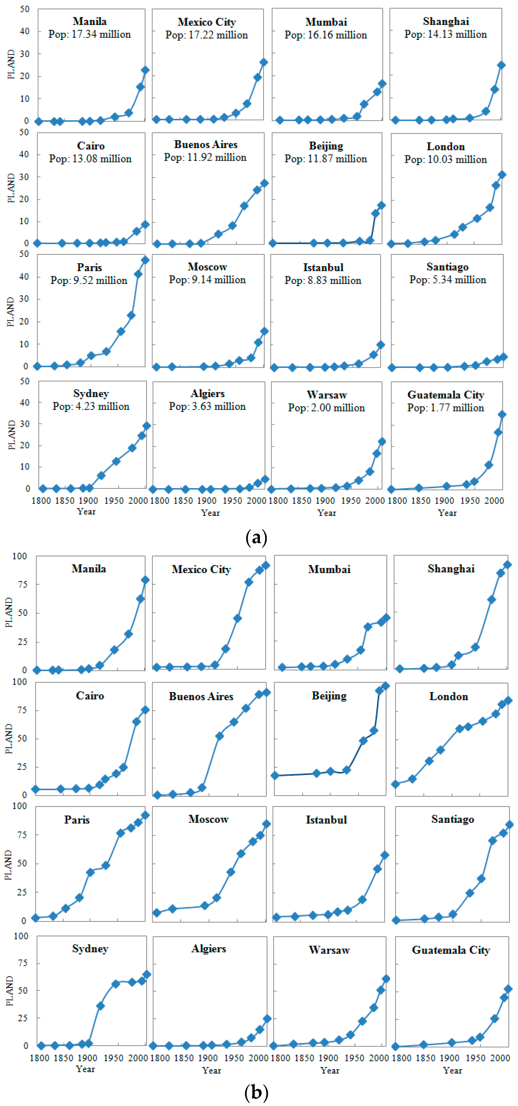
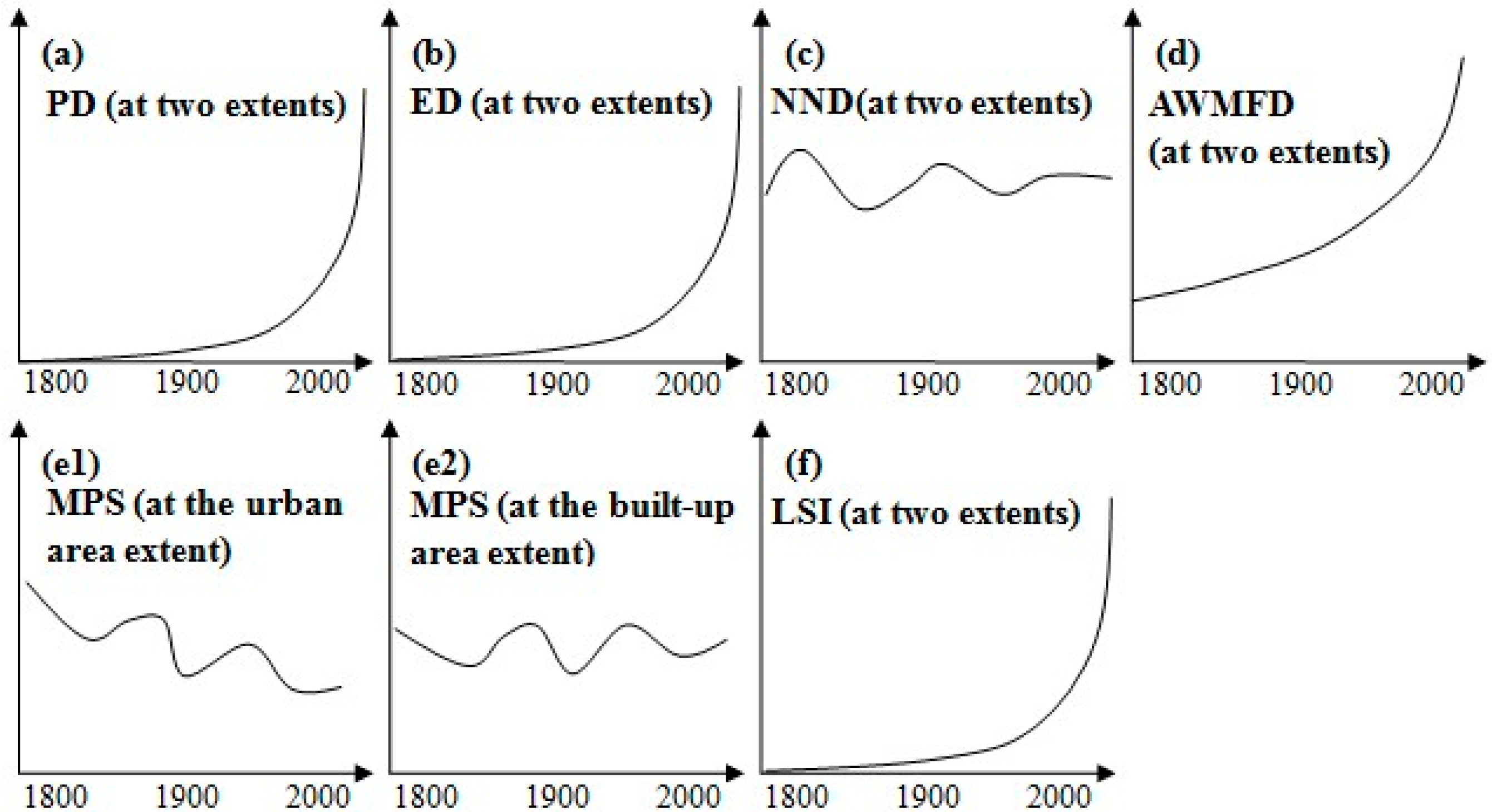
3.1. Changes in the Spatial Pattern of the Built-Up Area

The percentages of built-up areas (PLAND in the software of FRAGSTATS [37]) increased exponentially in all 16 cities from 1800–2000 at both extents (Figure 4). At the urban area extent, PLAND was less than 0.5% in each city in 1800, while this value was still less than 1% in most of the cities in 1900 (Figure 4a). In 2000, PLAND was close to or greater than 5% in all of the cities (Figure 4a). The increase of PLAND from 1900–2000 was more than five-times the increase from 1800–1900 in all of the cities (Figure 4a). In addition, PLAND was less than 25% at the built-up area extent in 1800, while it was close to 100% in most cases in 2000 (Figure 4b). This increase of PLAND mainly occurred after 1900 (Figure 4b).

Figure 4. Changes in the percentage of the built-up area (PLAND) in the 16 study cities from 1800–2000 at the two extents: (a) the urban area; and (b) the built-up area. The study cities are ordered by the urban population in 2000.

Figure 4. Changes in the percentage of the built-up area (PLAND) in the 16 study cities from 1800–2000 at the two extents: (a) the urban area; and (b) the built-up area. The study cities are ordered by the urban population in 2000.

PD, ED, LSI and AWMFD of built-up areas generally increased during urbanization from 1800–2000 (Figure 5). The values of PD, ED and LSI were all close to zero in 1800, but increased to more than 2 num/km², 10 m/ha and 60, respectively, in 2000, with the largest increases occurring between the 1970s and the 1990s for most of the cities (Figures S1a, S2a and S6a in Supplementary S3). The values of AWMFD increased from about 1.1 in 1800 to nearly 1.4 in 2000 in most of the cities (Figure S4a in Supplementary S3). At the built-up area extent, PD, ED, LSI and AWMFD also showed increasing trends from 1800–2000 in general (Figures S1b, S2b, S4b and S6b in Supplementary S3). In contrast, PD, ED and LSI of the built-up areas in Mumbai decreased from 1931–1955 at the two extents (Figures S1, S2 and S6 in Supplementary S3).

Figure 5. General trends of landscape metrics measuring the spatial pattern of the built-up area in the 16 study cities from 1800–2000 at the two extents (see Figures S1–S6 in Supplementary S3 for details). The X axis denotes the process of urbanization, and the Y axis denotes the value of landscape metrics measuring urbanization patterns. Landscape metrics include: patch density (PD), edge density (ED), mean Euclidean nearest neighbor distance (NND), area-weighted mean fractal dimension (AWMFD), mean patch size (MPS) and landscape shape index (LSI) (see Table 2 for details).

Figure 5. General trends of landscape metrics measuring the spatial pattern of the built-up area in the 16 study cities from 1800–2000 at the two extents (see Figures S1–S6 in Supplementary S3 for details). The X axis denotes the process of urbanization, and the Y axis denotes the value of landscape metrics measuring urbanization patterns. Landscape metrics include: patch density (PD), edge density (ED), mean Euclidean nearest neighbor distance (NND), area-weighted mean fractal dimension (AWMFD), mean patch size (MPS) and landscape shape index (LSI) (see Table 2 for details).

Two metrics, MPS and NND, changed as wave-shaped patterns from 1800–2000 (Figure 5). Specifically, the MPS revealed fluctuating changes with a general decreasing trend from 1800–2000 at the urban area extent; the values decreased from near 100 ha to less than 10 ha in most of the cities (Figure 5e1 and Figure S5a in Supplementary S3). At the built-up area extent, the values of MPS changed slightly between 1800 and 2000 (Figure 5e2 and Figure S5b in Supplementary S3). Furthermore, NND also changed a little, with values of about 100 m, between 1800 and 2000, in most of the cities at the two extents (Figure 5c and Figure S3 in Supplementary S3).

All three urban growth modes, infilling, edge expansion and leapfrog development, occurred simultaneously during urbanization, with changing relative dominance over time (Figure 6). Specifically, the proportions of the numbers and the areas of new urban patches for each growth mode both varied considerably among different time periods (Figure 6). Generally, leapfrog and infilling had a tendency to interchange their relative dominance, while edge expansion kept its importance in both the patch number and the patch area (Figure 6).

Figure 6. Changes in the relative dominance of three growth modes of urbanization (infilling, edge expansion and leapfrog) from 1800–2000 at the urban area extent (a) and the built-up area extent (b).

Figure 6. Changes in the relative dominance of three growth modes of urbanization (infilling, edge expansion and leapfrog) from 1800–2000 at the urban area extent (a) and the built-up area extent (b).

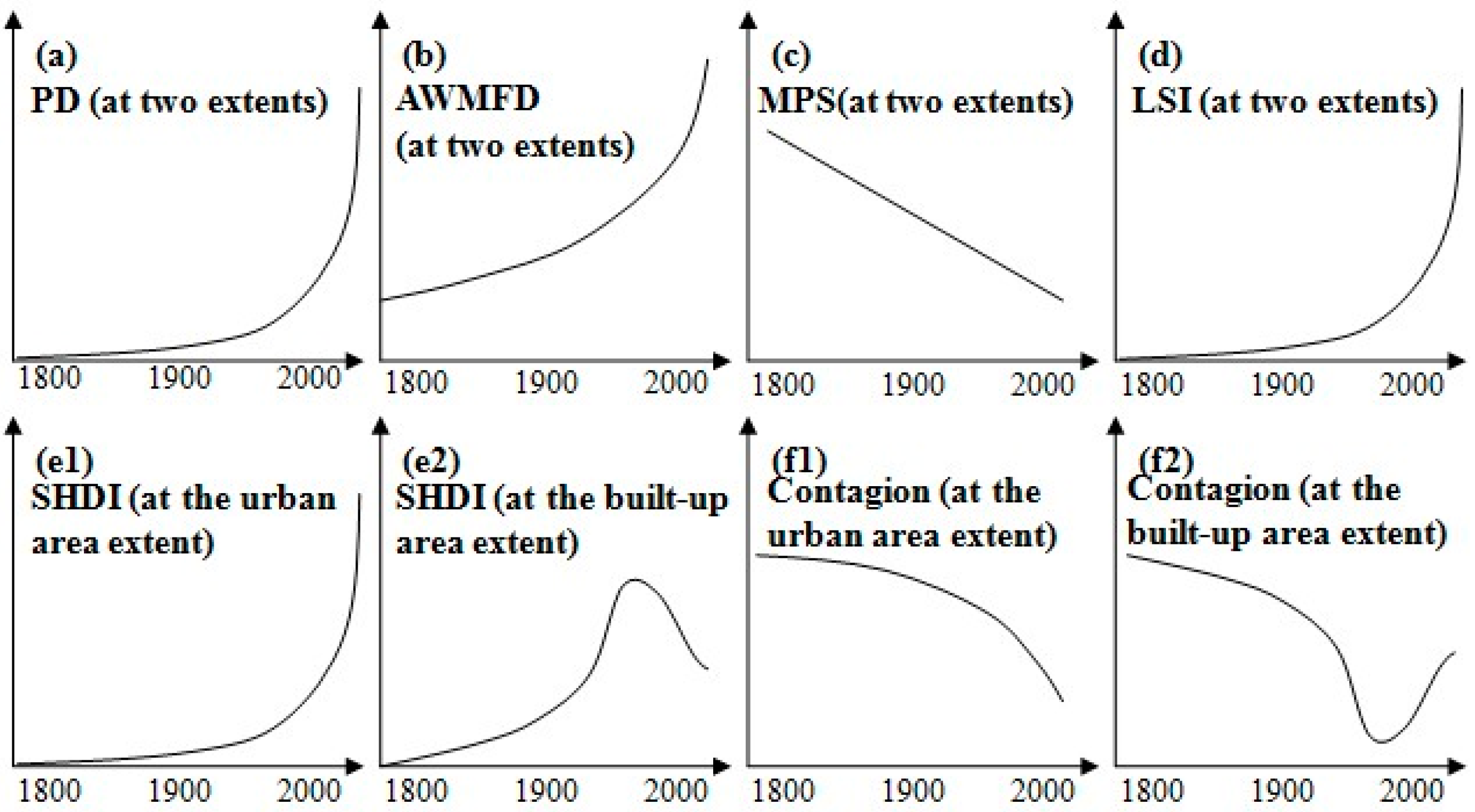
3.2. Changes in the Spatial Pattern of the Whole Urban Landscape

Among the four landscape metrics showing monotonic trends, PD, AWMFD and LSI increased, while MPS decreased during urbanization from 1800–2000 (Figure 7). Specifically, the increases of PD, AWMFD and LSI mainly took place after 1900. The values of PD increased from less than 1 num/km² in 1900 to more than 4 num/km² at the urban area extent and to above 10 num/km² at the built-up area extent in 2000 in most cases (Figure S7 in Supplementary S3). The values of AWMFD increased from less than 1.1 in 1900 to about 1.3 in 2000 at the two extents in general (Figure S8 in Supplementary S3). LSI commonly increased from about zero in 1900 to greater than 15 in 2000 at the two extents (Figure S10 in Supplementary S3). In contrast to the increases in PD, AWMFD and LSI, MPS decreased from above 1000 ha in 1800 to below 10 ha in 2000 at the urban area extent and declined from more than 100 ha in 1800 to less than 10 ha in 2000 at the built-up area extent in most of the cities (Figure S9 in Supplementary S3). In addition to the general trends, the decreases of PD, AWMFD and LSI and the increases of MPS were found at the two extents for Mumbai during the period of 1931–1955 (Figures S7–S10 in Supplementary S3).

Figure 7. General trends of landscape metrics measuring the spatial pattern of the whole urban landscape in the 16 study cities from 1800–2000 at the two extents (see Figures S7–S12 in Supplementary S3 for details). The X axis denotes the process of urbanization, and the Y axis denotes the value of landscape metrics measuring urbanization patterns. Landscape metrics include: patch density (PD), area-weighted mean fractal dimension (AWMFD), mean patch size (MPS), landscape shape index (LSI), Shannon’s diversity index (SHDI) and contagion (see Table 2 for details).

Figure 7. General trends of landscape metrics measuring the spatial pattern of the whole urban landscape in the 16 study cities from 1800–2000 at the two extents (see Figures S7–S12 in Supplementary S3 for details). The X axis denotes the process of urbanization, and the Y axis denotes the value of landscape metrics measuring urbanization patterns. Landscape metrics include: patch density (PD), area-weighted mean fractal dimension (AWMFD), mean patch size (MPS), landscape shape index (LSI), Shannon’s diversity index (SHDI) and contagion (see Table 2 for details).

Changes in SHDI and contagion were generally different between the two extents (Figure 7e–f and Figures S11 and S12 in Supplementary S3). At the urban area extent, changes in the two metrics showed monotonic trends in most cases (Figures S11a and S12a in Supplementary S3). To be specific, SHDI increased from circa zero in 1800 to above 0.2 in 2000 (Figure S11a in Supplementary S3), and contagion decreased from about 100 in 1800 to below 80 in 2000 (Figure S12a in Supplementary S3). At the built-up area extent, non-monotonic trends were generally found in changes of SHDI and contagion, and the thresholds of SHDI (about 0.7) and contagion (about 25) were respectively found in the same year in most of the cities (Figures S11b and S12b in Supplementary S3). Before approaching the corresponding thresholds, SHDI continuously increased, and contagion decreased, while they changed directions after reaching their thresholds, resulting in somewhat mirror images between SHDI and contagion (Figures S11b and S12b in Supplementary S3). In addition to the hump-shaped patterns and the U-shaped patterns, SHDI and contagion showed monotonic trends from 1800–2000 at the built-up area extent in Algiers (Figures S11b and S12b in Supplementary S3).

4. Discussion

4.1. Generalities and Idiosyncrasies in Urbanization Patterns

All 16 cities had experienced an exponential increase of built-up areas, resulting in dramatic changes in spatial patterns from 1800–2000. Specifically, the values of PLAND, PD, ED, LSI and AWMFD of the built-up areas all increased from 1800–2000 (Figure 5); changes in MPS and NND of the built-up areas, however, both revealed wave-shaped patterns (Figure 5). In the same period, the PD, AWMFD and LSI of the whole landscapes increased, as well, while the values of MPS decreased at the landscape level (Figure 7a–d). However, changes in SHDI and contagion differed between the two extents (Figure 7e–f). SHDI increased continuously, and contagion decreased monotonically at the urban area extent, while SHDI and contagion showed, respectively, a hump-shaped pattern and a U-shaped pattern at the built-up area extent (Figure 7e–f).

Cities in the same world region often revealed similar urbanization patterns, which usually varied slightly among different regions (Figure S13 in Supplementary S3). For instance, obvious increases of PLAND were found after the 1970s in the cities in Eastern Asia (i.e., Shanghai and Beijing), which were found after the 1950s in the cities in Central America (i.e., Mexico City and Guatemala City) and after the 1880s in the cities in Northern/Western Europe (i.e., London and Paris) (Figure S13 in Supplementary S3). In addition, the increases of PLAND in the cities in Northern Africa (i.e., Cairo and Algiers) were much less than the values in most cities in other regions (Figure S13 in Supplementary S3). The variation of urbanization patterns may result from the different urbanization levels among world regions.

The different patterns of changes mentioned above indicate that the choice of landscape metrics and the scale of analysis matter in charactering spatiotemporal patterns of urbanization [9,10,21,34]. NND of the built-up areas changed little between 1800 and 2000, which may be attributable to the distinguishing feature of urban growth that new urban patches were commonly built near existing urban patches [39] (Figure 5c); even though PD continued to increase, NND was not likely to change. Moreover, all of the changes in landscape metrics resulted from the integration of three urban growth modes: infilling, edge expansion and leapfrog development, with changing relative dominance over time (Figure 6). During the urbanization from 1800–2000, all of the three urban growth modes occurred simultaneously, while infilling and leapfrog generally showed opposite trends: when infilling increased its share in the number or the area of new urban patches, the corresponding value of leapfrog decreased, and vice versa (Figure 6). In addition to the alternation of the dominance of infilling and leapfrog, edge expansion remained relatively important during urbanization (Figure 6).

Besides the general patterns of urbanization, some idiosyncrasies also existed in several cities. For instance, PD, ED, LSI and AWMFD all decreased in Mumbai in the period of 1931–1955 at both extents (Figures S1, S2, S4 and S6 in Supplementary S3), and SHDI and contagion changed monotonically in Algiers from 1800–2000 at the built-up area extent (Figures S11b and S12b in Supplementary S3). The monotonic changes in SHDI and contagion in Algiers were apparently due to the much slower urbanization rate (Figure 4), with less than 25% of the built-up area as urban land in 2000, as compared to greater than 50% for other cities (Figure 4b). In addition, the unusual pattern of urbanization in Mumbai in the period of 1931–1955 may be attributable to the land policy change after the independence of India in 1947 [40].

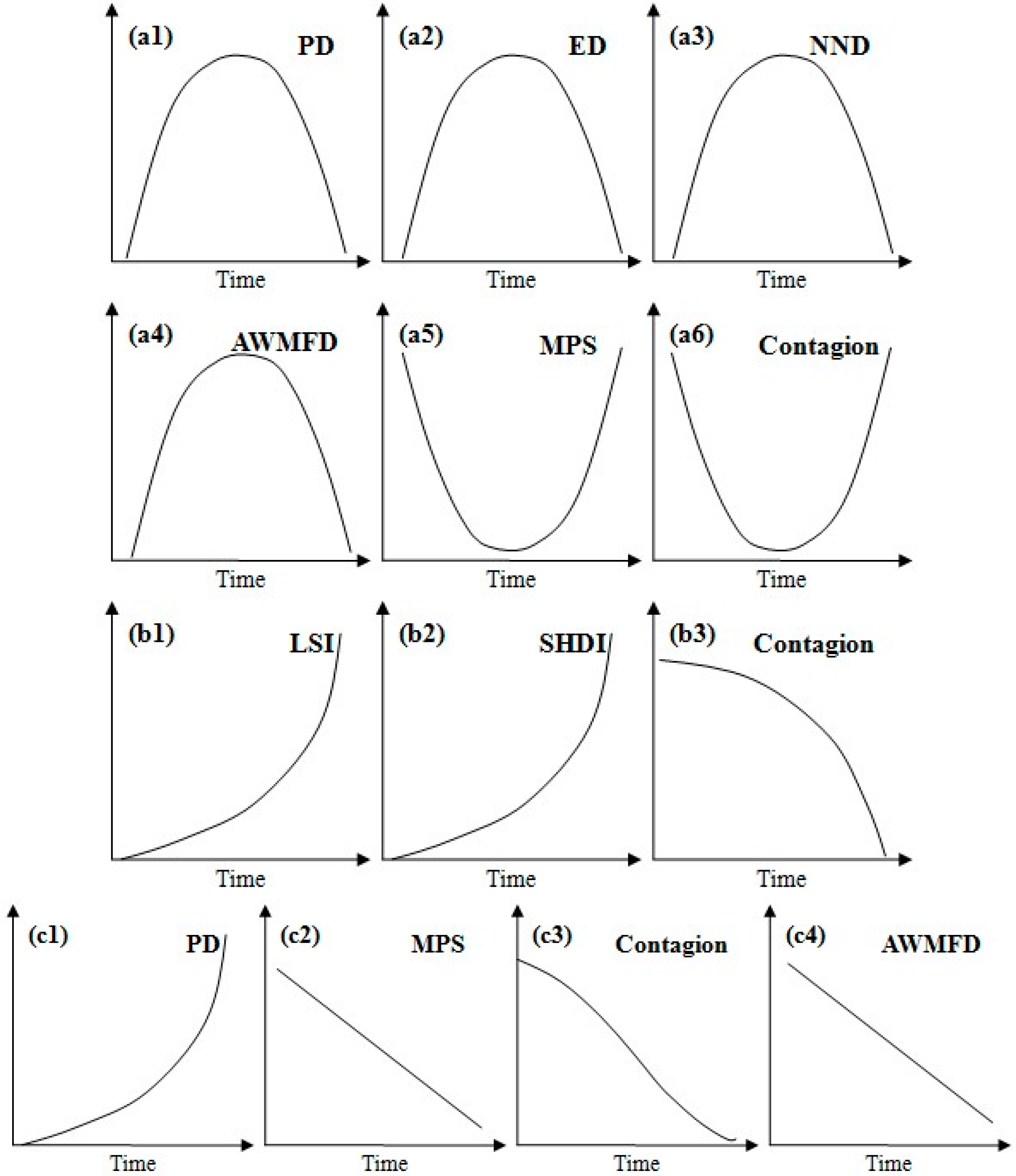
4.2. Testing Hypotheses of Urbanization Patterns

4.2.1. The Diffusion and Coalescence Hypothesis

Diffusion here refers to the urban growth mode of leapfrogging, while coalescence represents the commingling of infilling and edge expansion [18,19,35]. According to Dietzel et al. [18,19], this hypothesis can be translated into testable temporal patterns of landscape metrics: the urban land area increases monotonically; PD, ED, AWMFD and NND of urban patches increase first, then peak at different times and, finally, decrease, exhibiting unimodal shapes (Figure 1a); MPS of urban patches and contagion of the whole landscape are highest at the beginning of the diffusion process and the end of the coalescence process and reach their lowest values in between, thus exhibiting somewhat mirror images of PD, ED, AWMFD and NND (Figure 1a). Our results indicate that the “diffusion and coalescence” hypothesis may manifest in many cities during a relatively short duration, but is too simplistic over a few centuries. The wave-shaped trends of MPS and NND at the two extents (Figure 5c,e) and the unimodal-shaped trends of contagion at the built-up area extent (Figure 7f) supported this hypothesis. However, in terms of either the number or the area of new urban patches, all three urban growth modes (i.e., infilling, edge expansion and leapfrog) occurred simultaneously during urbanization (Figure 6); no single process of diffusion or coalescence occurred alone during urbanization.

4.2.2. The Three Growth Modes Hypothesis

As already mentioned above, our results are more consistent with the three growth modes hypothesis than the diffusion-coalescence hypothesis. In a study of the central Yangtze River Delta region, China, Li et al. [20] concluded that “it is more plausible to view urbanization as a spiraling process that involves three growth modes of leapfrogging, edge-expanding, and infilling”, and that “leapfrog and infilling tend to alternate in their relative dominance while edge-expansion is likely to maintain its importance throughout much of the urbanization process”. Our results of four world cities fully corroborate this hypothesis (Figure 6).

4.2.3. The Landscape Modification Gradient Hypothesis

Forman and Godron [27] postulated that PD and the regularity of patch shape would increase, while MPS and landscape connectivity would decrease, along a landscape modification gradient. From a time-for-space perspective, the natural-to-urban gradient in space can be approximated by the temporal urbanization pattern of cities (Figure 1c). Taking such a perspective, our results of PD, MPS and landscape connectivity generally support the landscape modification gradient hypothesis (Figure 7a,c,f), assuming that landscape connectivity is positively related to contagion and negatively to PD [10]. However, our study shows that the regularity of patch shape, conversely related to AWMFD, decreased as urbanization progressed for the 16 cities (Figure 7b).

4.2.4. The Diversity-Complexity Hypothesis

According to Wu et al. [10,21,22,23], as urbanization unfolds, LSI and SHDI increase, whereas contagion decreases, i.e., urbanization increases the compositional diversity and structural complexity (Figure 1b). In this study, we found that at the urban area extent, LSI and SHDI increased, whereas contagion decreased, monotonically, confirming the diversity-complexity hypothesis (Figure 7d,e1,f1). At the smaller extent of the urban core area, however, the monotonic changes may hit the ceiling or change directions when much of the landscape is urbanized (Figure 7e2,f2).

4.3. Suggestions for Choosing Landscape Metrics in Quantifying Urbanization Patterns

In this study, we selected landscape metrics to quantify urbanization patterns based on two principles. First, the metrics were used in the four prominent hypotheses of urbanization patterns [10,18,19,20,21,22,23,27]. Second, the metrics measured urbanization patterns well according to our previous study in Phoenix and Las Vegas [10]. Specifically, seven class-level metrics (PLAND, PD, ED, NND, MPS, AWMFD and LSI) and six landscape-level metrics (PD, MPS, AWMFD, LSI, SHDI and contagion) were used.

It is well known that many landscape metrics are closely related, resulting in redundancy in quantifying landscape patterns [37]. In our research, we also found that several metrics showed similar or inverse trends, which were seemingly related. Among class-level metrics, PD, ED, AWMFD and LSI showed similar trends during urbanization (Figure 5). Among the landscape-level metrics, PD, AWMFD and LSI represented similar trends, while SHDI and contagion showed inverse trends (Figure 7). These related metrics may cause redundancy in quantifying urbanization patterns.

To quantify landscape patterns without redundancy, eliminating related metrics is needed. To achieve this, Riitters et al. [41] identified six common dimensions of pattern and structure (i.e., composite measures of average patch compaction, overall image texture, average patch shape, patch perimeter area scaling, the number of attribute classes and large patch density area scaling) and found that the information of 55 metrics could be reduced to six univariate metrics (i.e., average perimeter-area ratio, contagion, standardized patch shape, patch perimeter area scaling, the number of attribute classes and large patch density area scaling) to represent these dimensions in a simpler way. Frohn and Hao [42] divided 16 metrics into four individual groups, including class metrics, shape metrics, patch metrics and edge metrics, and found that LSI, square pixel (SqP), ED, PD and NND were appropriate to measure spatial aggregation. According to the previous studies, we suggested that at least one of the metrics representing different aspects of landscape pattern should be selected, and two or three metrics describing patterns in the same aspect were recommended to be calculated to confirm each other. Thus, six metrics (i.e., PLAND, PD, LSI, MPS, NND and contagion), which described urbanization patterns in various aspects, should be selected. In addition, ED, AWMFD and SHDI were recommended to confirm these in quantifying urbanization patterns.

5. Conclusions

Cities differ in many ways, from climate to architecture, ecology, economy and culture. While idiosyncratic differences abound, our study of 16 world cities reveals several general spatiotemporal patterns of urbanization common to seemingly disparate cities. First, urbanization generally leads to an increasingly diverse and complex cityscape. As Wu et al. [10,21,22,23] put it, as urbanization continued to unfold, “landscapes became increasingly more diverse in land use, more fragmented in structure, and more complex in shape”. Second, the spatial dynamics of urbanization often operates through three growth modes, infilling, edge-expanding and leapfrogging, which commingle, but with shifting dominance [20]. Third, behind these general patterns are complex details that distinguish individual cities, which are closely related to specific environmental and socioeconomic settings. Our study demonstrates these patterns, for the first time, on long-term and global scales. These global trends help us better understand the patterns and processes of urbanization and suggest some fundamental problems with global urbanization so far. For example, urbanization around the world has led to increasing landscape fragmentation that has negative impacts on ecosystem function and services, urban sprawl that encroaches into agricultural land and natural habitat and homogenizing urban morphology, which diminishes the cultural identities of cities. Future urban studies need to consider both generalities and idiosyncrasies and relate them directly to measures of urban sustainability [5].

References

1. Forman, R.T.T. The urban region: Natural systems in our place, our nourishment, our home range, our future. Landsc. Ecol. 2008, 23, 251–253. [Google Scholar] [CrossRef]
2. Grimm, N.B.; Faeth, S.H.; Golubiewski, N.E.; Redman, C.L.; Wu, J.; Bai, X.; Briggs, J.M. Global change and the ecology of cities. Science 2008, 319, 756–760. [Google Scholar] [CrossRef] [PubMed]
3. Schneider, A.; Mertes, C.M.; Tatem, A.J.; Tan, B.; Sulla-Menashe, D.; Graves, S.J.; Patel, N.N.; Horton, J.A.; Gaughan, A.E.; Rollo, J.T.; et al. A new urban landscape in east-southeast asia, 2000–2010. Environ. Res. Lett. 2015, 10, 034002. [Google Scholar] [CrossRef]
4. Wu, J. Urban sustainability: An inevitable goal of landscape research. Landsc. Ecol. 2010, 25, 1–4. [Google Scholar] [CrossRef]
5. Wu, J. Urban ecology and sustainability: The state-of-the-science and future directions. Landsc. Urban Plan. 2014, 125, 209–221. [Google Scholar] [CrossRef]
6. Zhou, Y.Y.; Smith, S.J.; Zhao, K.G.; Imhoff, M.; Thomson, A.; Bond-Lamberty, B.; Asrar, G.; Zhang, X.S.; He, C.Y.; Elvidge, C.D. A global map of urban extent from nightlights. Environ.Res. Lett. 2015, 10, 054011. [Google Scholar] [CrossRef]
7. UN. World Urbanization Prospects: The 2011 Revision; United Nations, Department of Economic and Social Affairs, Population Division: New York, NY, USA, 2012. [Google Scholar]
8. Angel, S.; Parent, J.; Civco, D.L.; Blei, A.; Potere, D. The dimensions of global urban expansion: Estimates and projections of all countries, 2000–2050. Prog. Plan. 2011, 75, 53–107. [Google Scholar] [CrossRef]
9. Luck, M.; Wu, J. A gradient analysis of urban landscape pattern: A case study from the phoenix metropolitan region, arizona, USA. Landsc. Ecol. 2002, 17, 327–339. [Google Scholar] [CrossRef]
10. Wu, J.; Jenerette, G.D.; Buyantuyev, A.; Redman, C.L. Quantifying spatiotemporal patterns of urbanization: The case of the two fastest growing metropolitan regions in the united states. Ecol. Complex. 2011, 8, 1–8. [Google Scholar] [CrossRef]
11. Angel, S.; Parent, J.; Civco, D.L. The fragmentation of urban landscapes: Global evidence of a key attribute of the spatial structure of cities, 1990–2000. Environ. Urban. 2012, 24, 249–283. [Google Scholar] [CrossRef]
12. Frolking, S.; Milliman, T.; Seto, K.C.; Friedl, M.A. A global fingerprint of macro-scale changes in urban structure from 1999 to 2009. Environ. Res. Let. 2013, 8, 024004. [Google Scholar] [CrossRef]
13. Taubenbock, H.; Esch, T.; Felbier, A.; Wiesner, M.; Roth, A.; Dech, S. Monitoring urbanization in mega cities from space. Remote Sens. Environ. 2012, 117, 162–176. [Google Scholar] [CrossRef]
14. Li, H.; Wei, Y.H.D.; Huang, Z.J. Urban land expansion and spatial dynamics in globalizing shanghai. Sustainability 2014, 6, 8856–8875. [Google Scholar] [CrossRef]
15. Lu, S.; Guan, X.; He, C.; Zhang, J. Spatio-temporal patterns and policy implications of urban land expansion in expansion in metropolitan areas: A case study of wuhan urban agglomeration, central China. Sustainability 2014, 6, 4723–4748. [Google Scholar] [CrossRef]
16. Gao, J.L.; Wei, Y.D.; Chen, W.; Yenneti, K. Urban land expansion and structural change in the yangtze river delta, China. Sustainability 2015, 7, 10281–10307. [Google Scholar] [CrossRef]
17. You, H. Quantifying urban fragmentation under economic transition in shanghai city, China. Sustainability 2016, 8, 21. [Google Scholar] [CrossRef]
18. Dietzel, C.; Herold, M.; Hemphill, J.J.; Clarke, K.C. Spatio-temporal dynamics in california’s central valley: Empirical links to urban theory. Int. J. Geogr. Inf. Sci. 2005, 19, 175–195. [Google Scholar] [CrossRef]
19. Dietzel, C.; Oguz, H.; Hemphill, J.J.; Clarke, K.C.; Gazulis, N. Diffusion and coalescence of the houston metropolitan area: Evidence supporting a new urban theory. Environ. B Plan. Des. 2005, 32, 231–246. [Google Scholar] [CrossRef]
20. Li, C.; Li, J.; Wu, J. Quantifying the speed, growth modes, and landscape pattern changes of urbanization: A hierarchical patch dynamics approach. Landsc. Ecol. 2013, 28, 1875–1888. [Google Scholar] [CrossRef]
21. Wu, J. Landscape Ecology: Pattern, Process, Scale, and Hierarchy; Higher Education Press: Beijing, China, 2000. [Google Scholar]
22. Wu, J. Modeling. In CAP-LTER 2001–2002 Annual Progress Report to NSF; 2002; Available online: http://caplter.asu.edu/docs/reports/2002AnnRept/2002CAPLTERAnnualReport.pdf (accessed on 31 December 2015).
23. Wu, J.; Jenerette, G.D.; David, J.L. Linking land-use change with ecosystem processes: A hierarchical patch dynamic model. In Integrated Land Use and Environmental Models—A Survey of Current Applications and Research; Guhathakurta, S., Ed.; Springer: Berlin, German, 2003. [Google Scholar]
24. Jenerette, G.D.; Potere, D. Global analysis and simulation of land-use change associated with urbanization. Landsc. Ecol. 2010, 25, 657–670. [Google Scholar] [CrossRef]
25. Schneider, A.; Woodcock, C.E. Compact, dispersed, fragmented, extensive? A comparison of urban growth in twenty-five global cities using remotely sensed data, pattern metrics and census information. Urban Stud. 2008, 45, 659–692. [Google Scholar] [CrossRef]
26. Seto, K.C.; Fragkias, M. Quantifying spatiotemporal patterns of urban land-use change in four cities of china with time series landscape metrics. Landsc. Ecol. 2005, 20, 871–888. [Google Scholar] [CrossRef]
27. Forman, R.T.T.; Godron, M. Landscape Ecology; Wiley: New York, NY, USA, 1986. [Google Scholar]
28. Lincoln Institute of Land Policy. Atlas of Urban Expansion. Available online: http://www.lincolninst.edu/subcenters/atlas-urban-expansion/ (accessed on 7 January 2014).
29. Angel, S.; Parent, J.; Civco, D.L.; Blei, A.M. The Persistent Decline of Urban Densities: Global and Historical Evidence of Sprawl; Lincoln Institute of Land Policy: Cambridge, MA, USA, 2010. [Google Scholar]
30. Zhang, Q.; Seto, K.C. Mapping urbanization dynamics at regional and global scales using multi-temporal dmsp/ols nighttime light data. Remote Sens. Environ. 2011, 115, 2320–2329. [Google Scholar] [CrossRef]
31. Liu, Z.; He, C.; Zhang, Q.; Huang, Q.; Yang, Y. Extracting the dynamics of urban expansion in china using dmsp-ols nighttime light data from 1992 to 2008. Landsc. Urban Plan. 2012, 106, 62–72. [Google Scholar] [CrossRef]
32. He, C.; Liu, Z.; Tian, J.; Ma, Q. Urban expansion dynamics and natural habitat loss in china: A multiscale landscape perspective. Glob. Chang. Biol. 2014, 20, 2886–2902. [Google Scholar] [CrossRef] [PubMed]
33. Liu, Z.; He, C.; Zhou, Y.; Wu, J. How much of the world’s land has been urbanized, really? A hierarchical framework for evading confusion. Landsc. Ecol. 2014, 29, 763–771. [Google Scholar] [CrossRef]
34. Wu, J. Effects of changing scale on landscape pattern analysis: Scaling relations. Landsc. Ecol. 2004, 19, 125–138. [Google Scholar] [CrossRef]
35. Liu, X.; Li, X.; Chen, Y.; Tan, Z.; Li, S.; Ai, B. A new landscape index for quantifying urban expansion using multi-temporal remotely sensed data. Landsc. Ecol. 2010, 25, 671–682. [Google Scholar] [CrossRef]
36. Weng, Y.C. Spatiotemporal changes of landscape pattern in response to urbanization. Landsc. Urban Plan. 2007, 81, 341–353. [Google Scholar] [CrossRef]
37. McGarigal, K.; Cushman, S.A.; Neel, M.C.; Ene, E. Fragstats: Spatial Pattern Analysis Program for Categorical Maps, 3.1st edn; University of Massachusetts: Amherst, MA, USA, 2002. [Google Scholar]
38. ESRI. Arcgis desktop: Release 10; Environmental Systems Research Institute: Redlands, CA, USA, 2011. [Google Scholar]
39. He, C.; Okada, N.; Zhang, Q.; Shi, P.; Li, J. Modelling dynamic urban expansion processes incorporating a potential model with cellular automata. Landsc.Urban Plan. 2008, 86, 79–91. [Google Scholar] [CrossRef]
40. Wissink, B. Enclave urbanism in mumbai: An actor-network-theory analysis of urban (dis)connection. Geoforum 2013, 47, 1–11. [Google Scholar] [CrossRef]
41. Riitters, K.H.; Oneill, R.V.; Hunsaker, C.T.; Wickham, J.D.; Yankee, D.H.; Timmins, S.P.; Jones, K.B.; Jackson, B.L. A factor-analysis of landscape pattern and structure metrics. Landsc. Ecol. 1995, 10, 23–39. [Google Scholar] [CrossRef]
42. Frohn, R.; Hao, Y. Landscape metric performance in analyzing two decades of deforestation in the amazon basin of rondonia, brazil. Remote Sens. Environ. 2006, 100, 237–251. [Google Scholar] [CrossRef]