
Analyzing Three-Decadal Patterns of Land Use/Land Cover Change and Regional Ecosystem Services at the Landscape Level: Case Study of Two Coastal Metropolitan Regions, Eastern China


Abstract
:1. Introduction
2. Materials and Methods
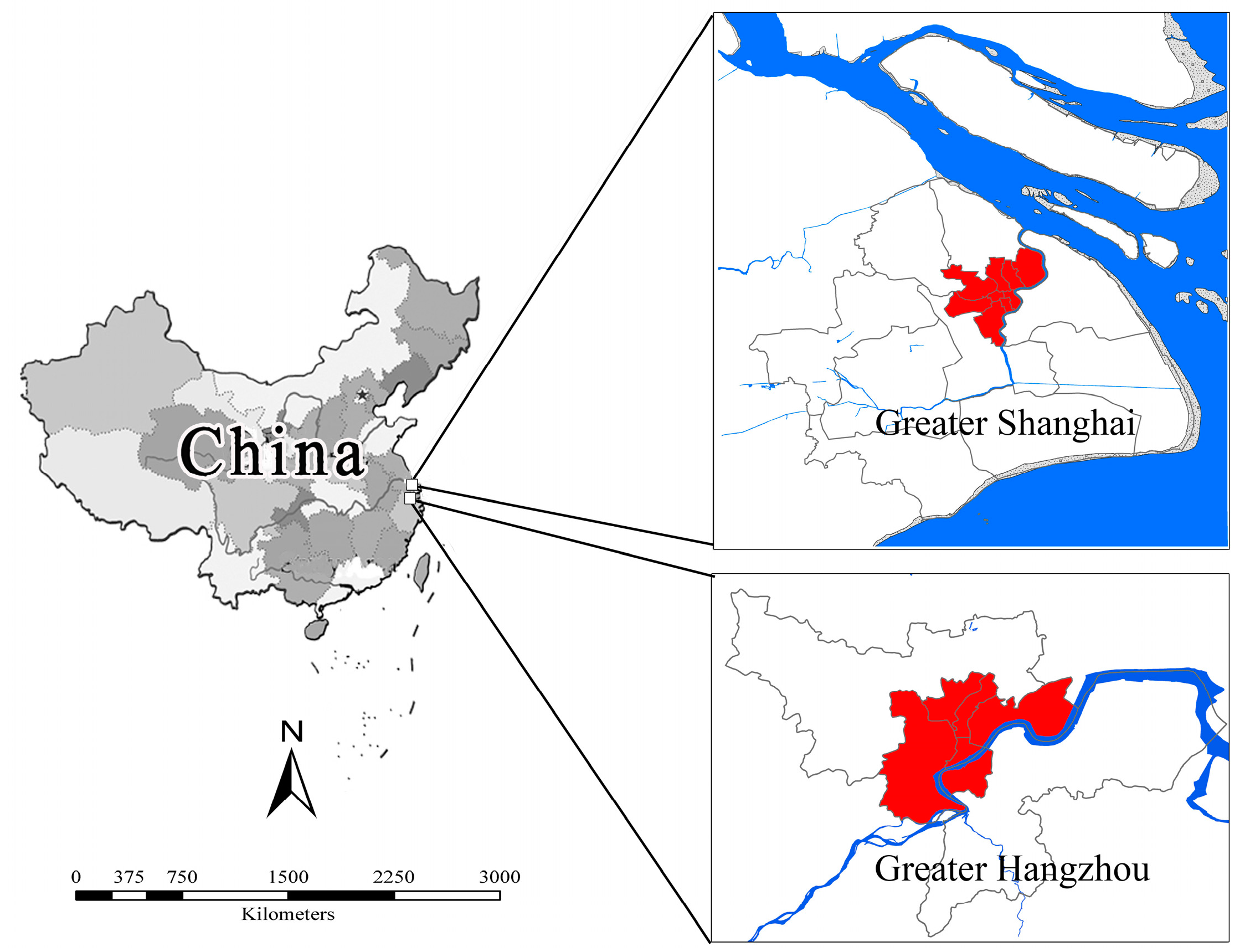
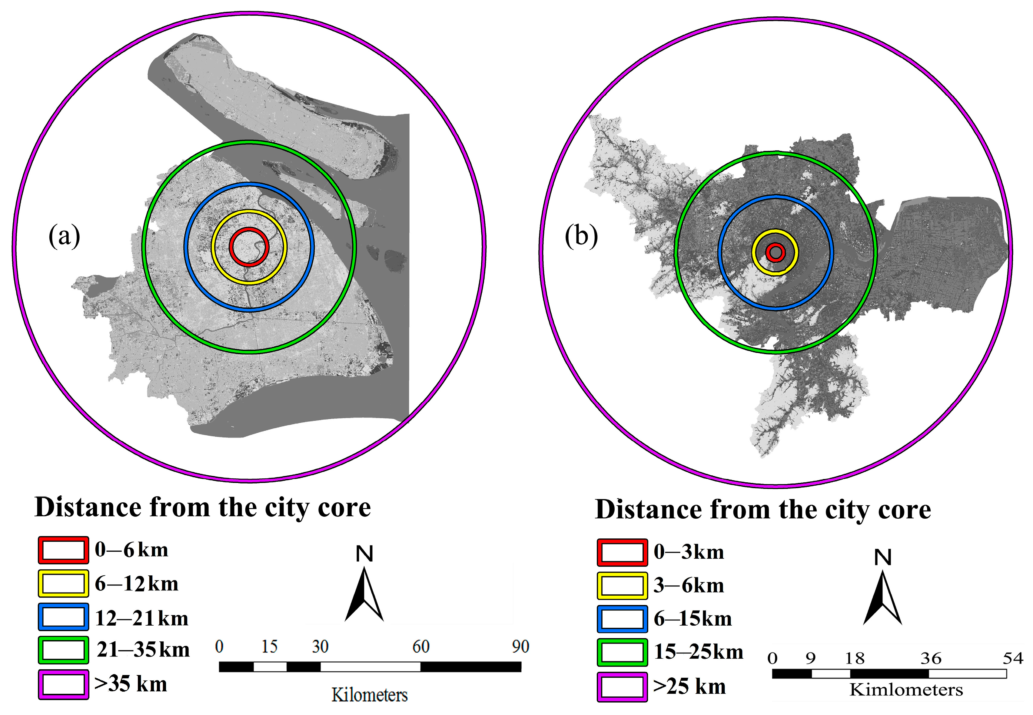
2.1. Study Areas
2.2. Data Sources
2.3. Satellite Imagery Preprocessing, Classification, Accuracy Assessment, and Post-Classification
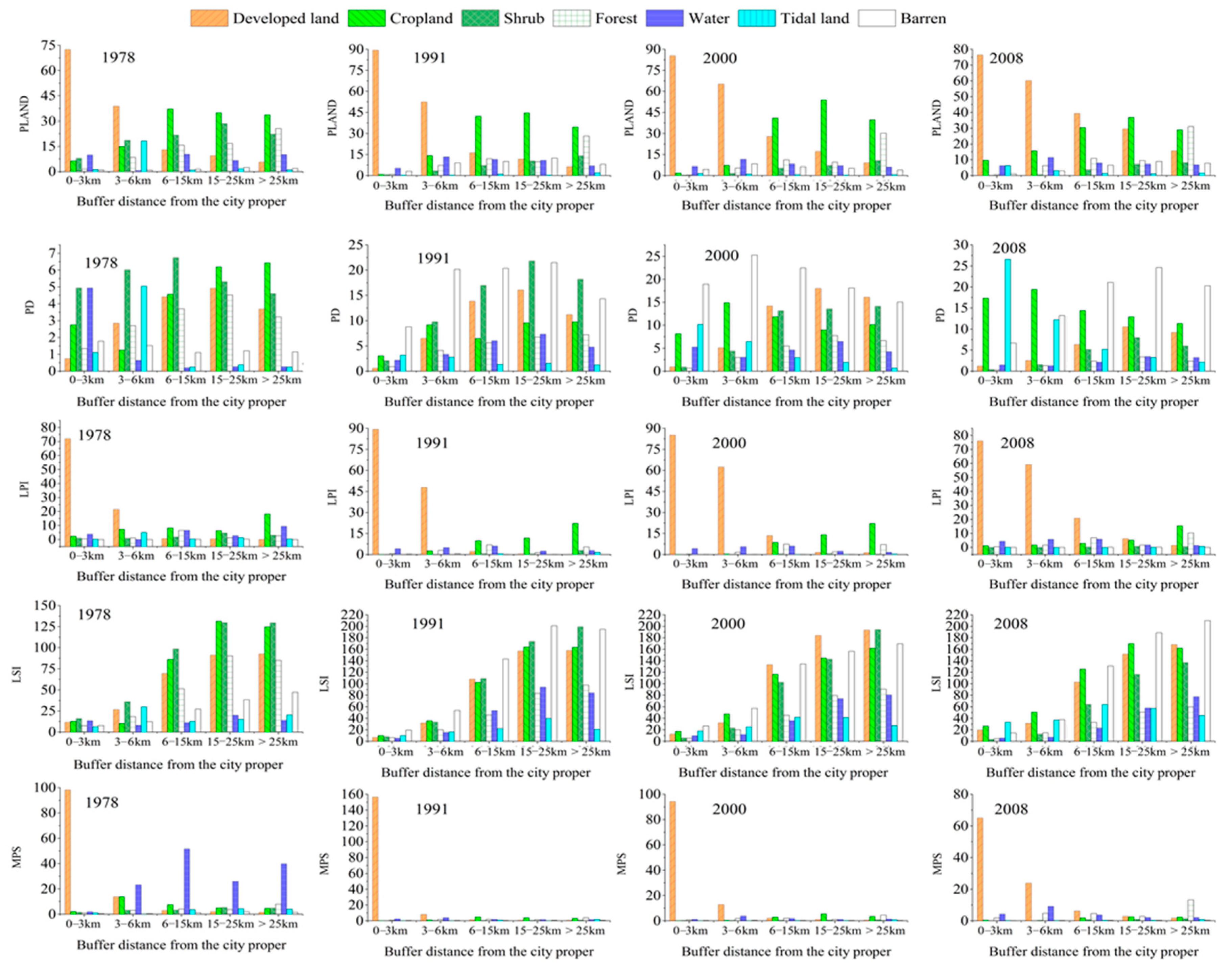
2.4. Computation of Class-Level Metrics for Measuring Landscape Fragmentation
2.5. Computation of Regional ESV
2.6. Statistical Analysis
3. Results
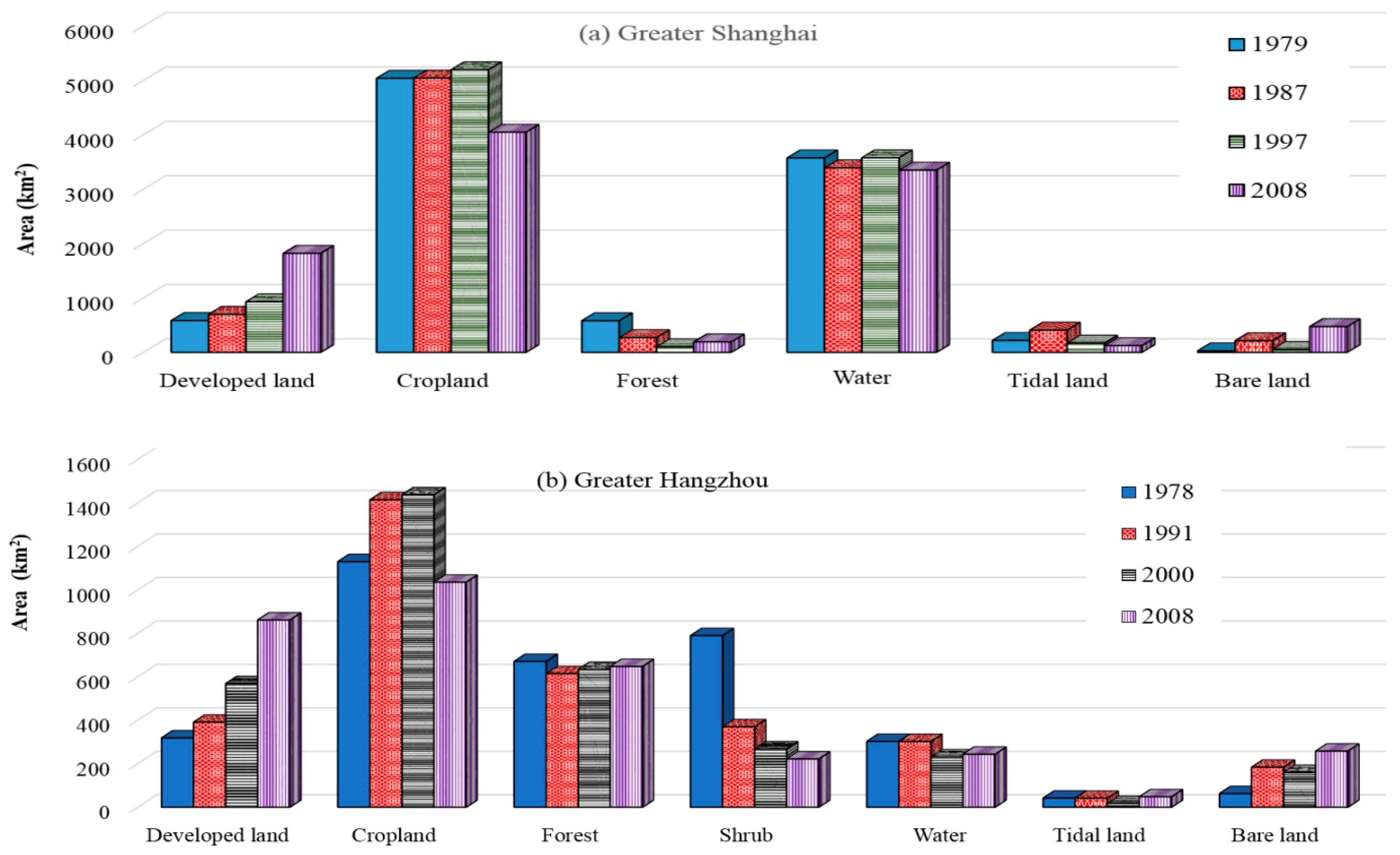
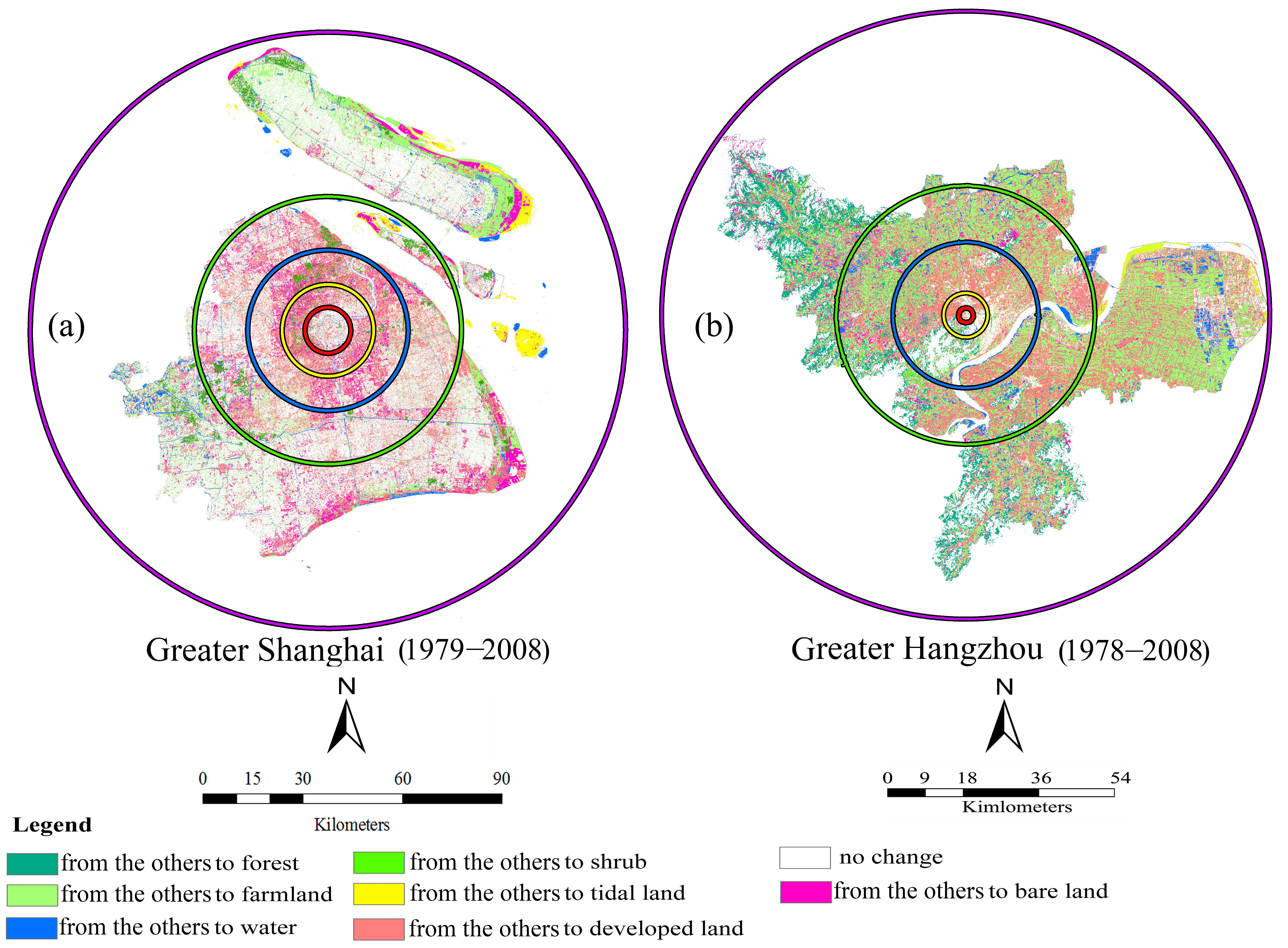
3.1. LULC Change
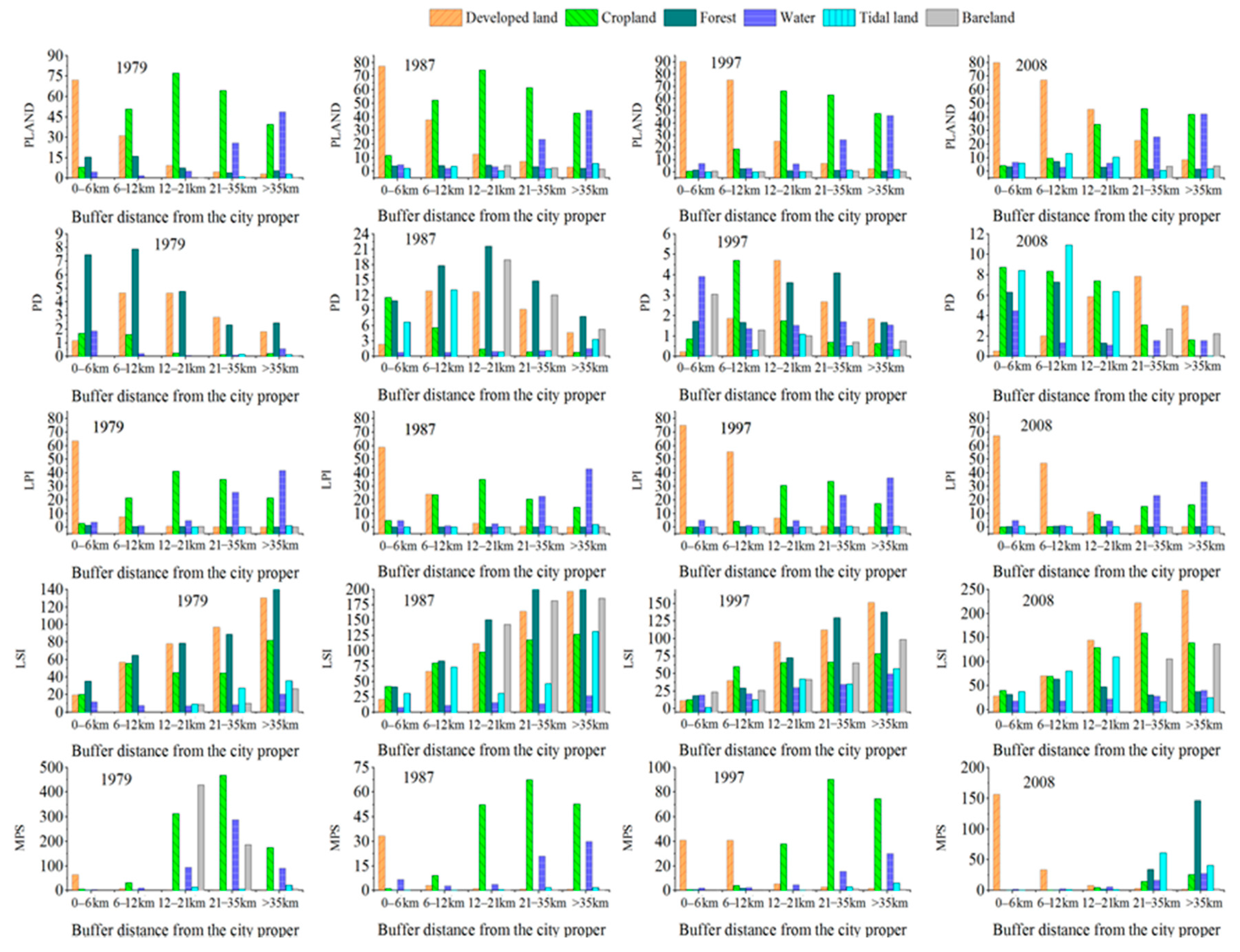
3.2. Variation of Class-Level Landscape Patterns
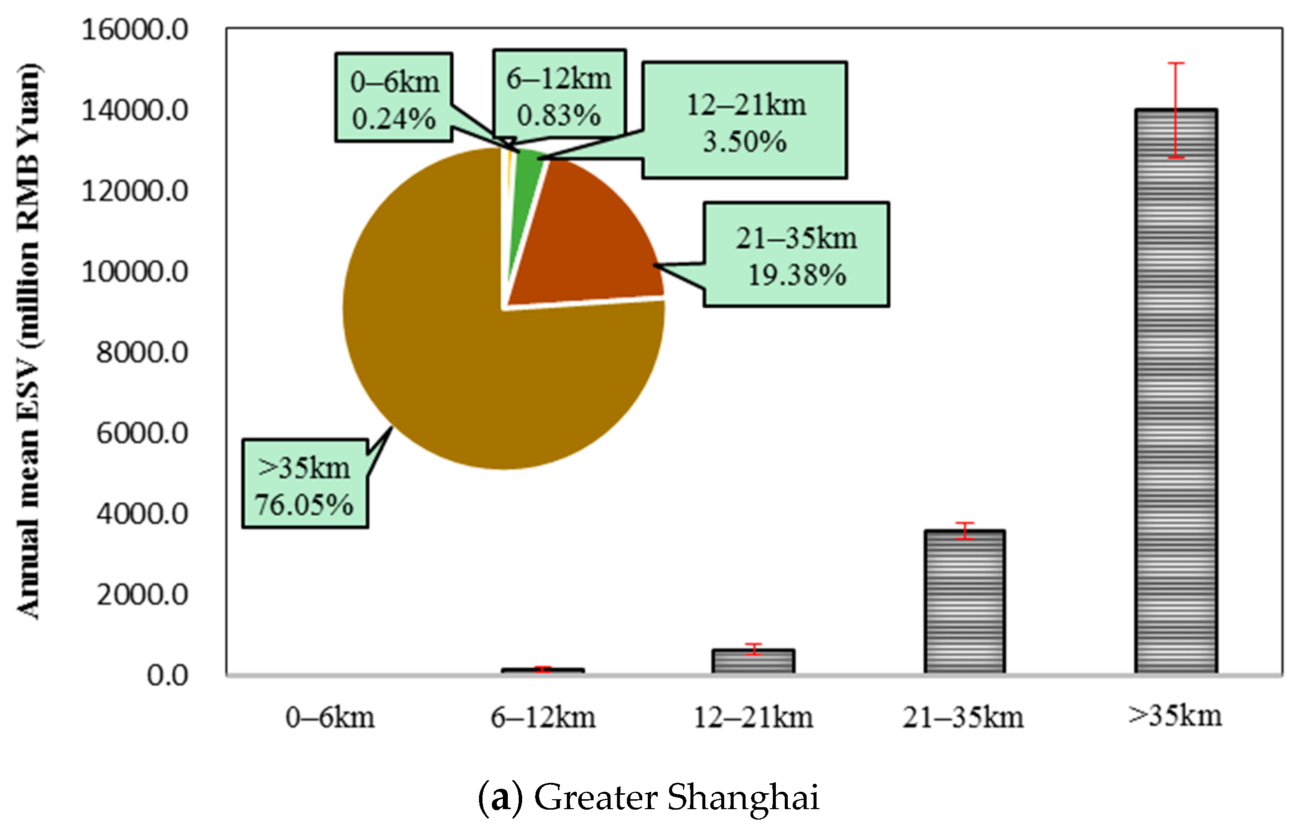
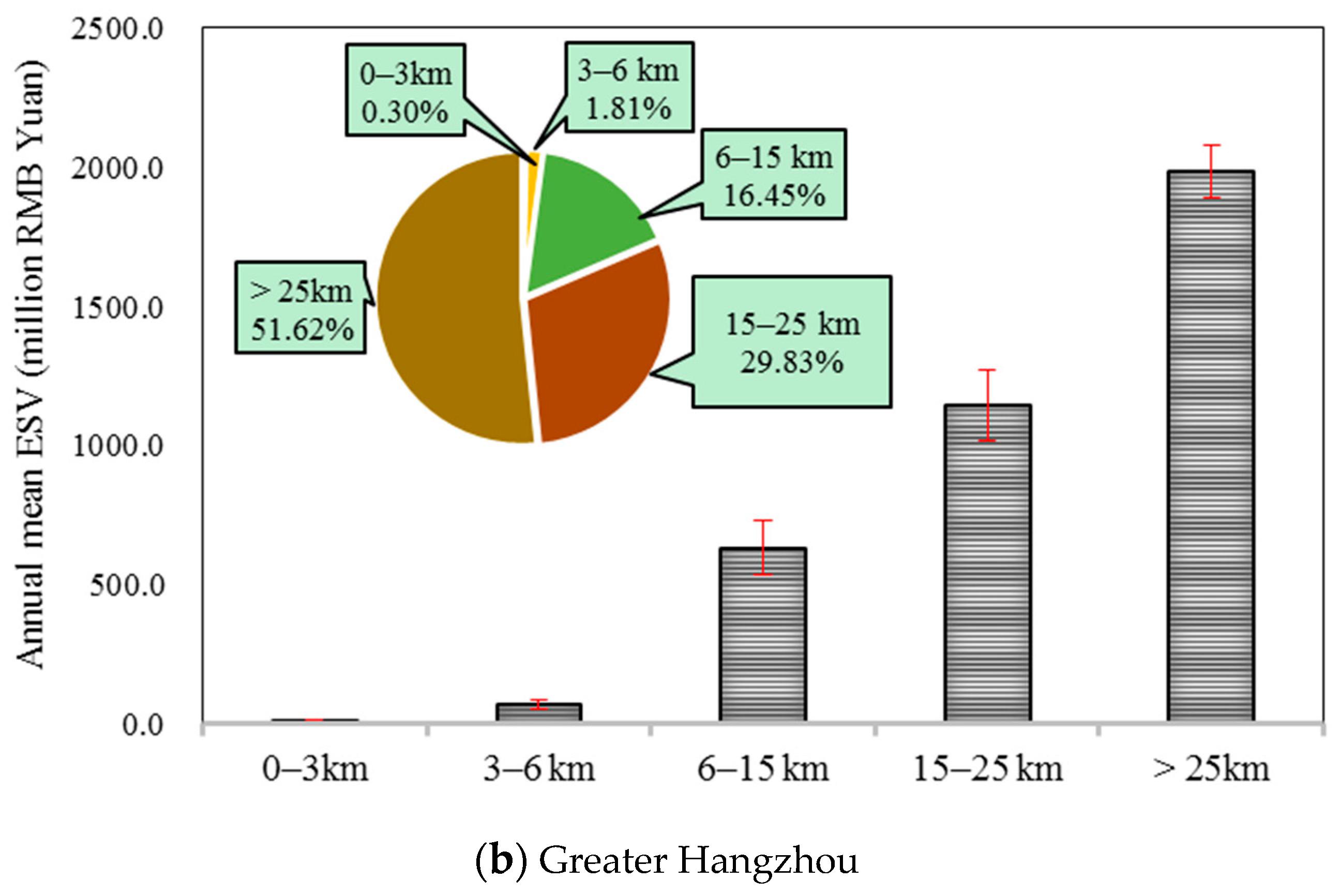
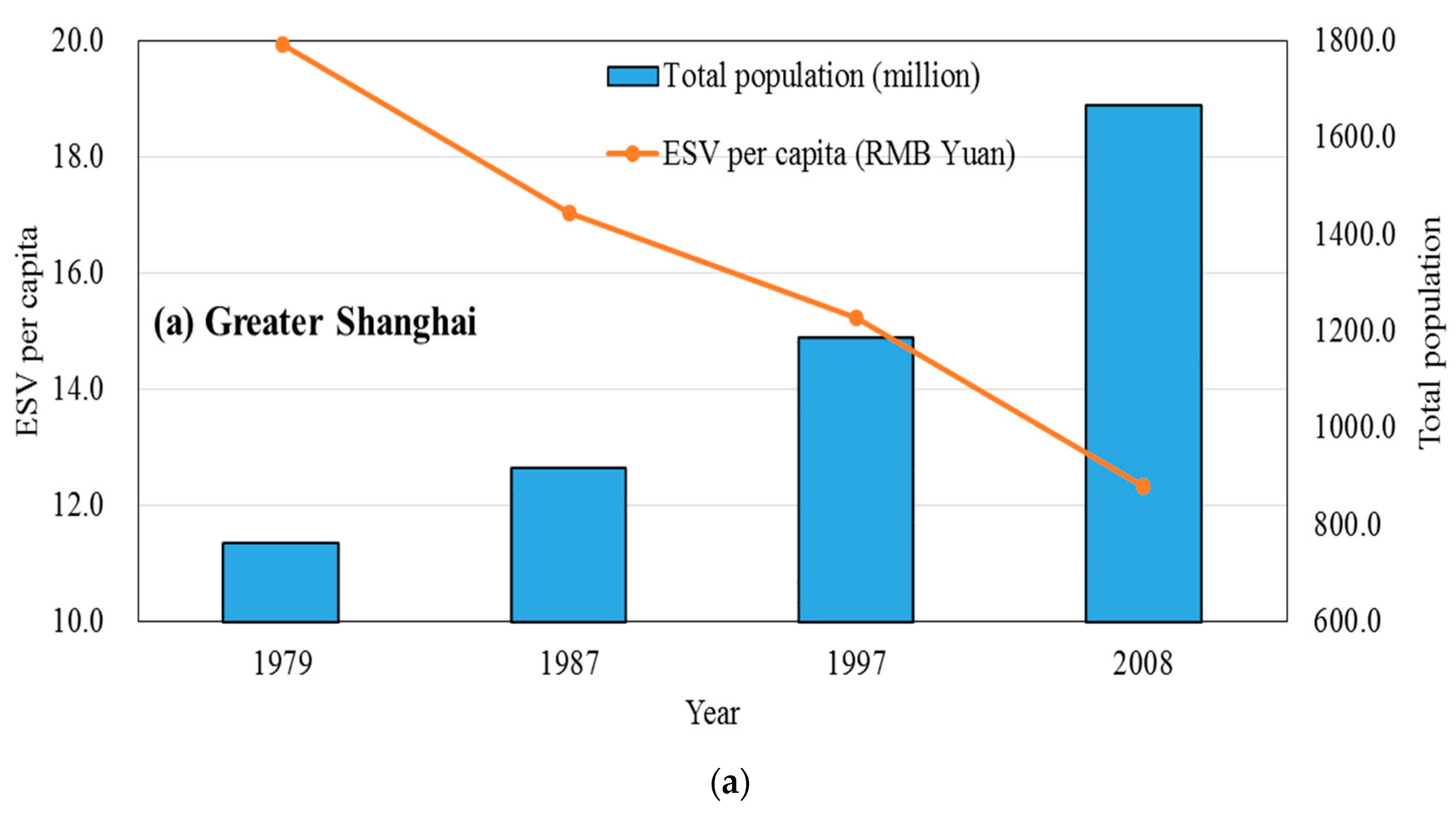
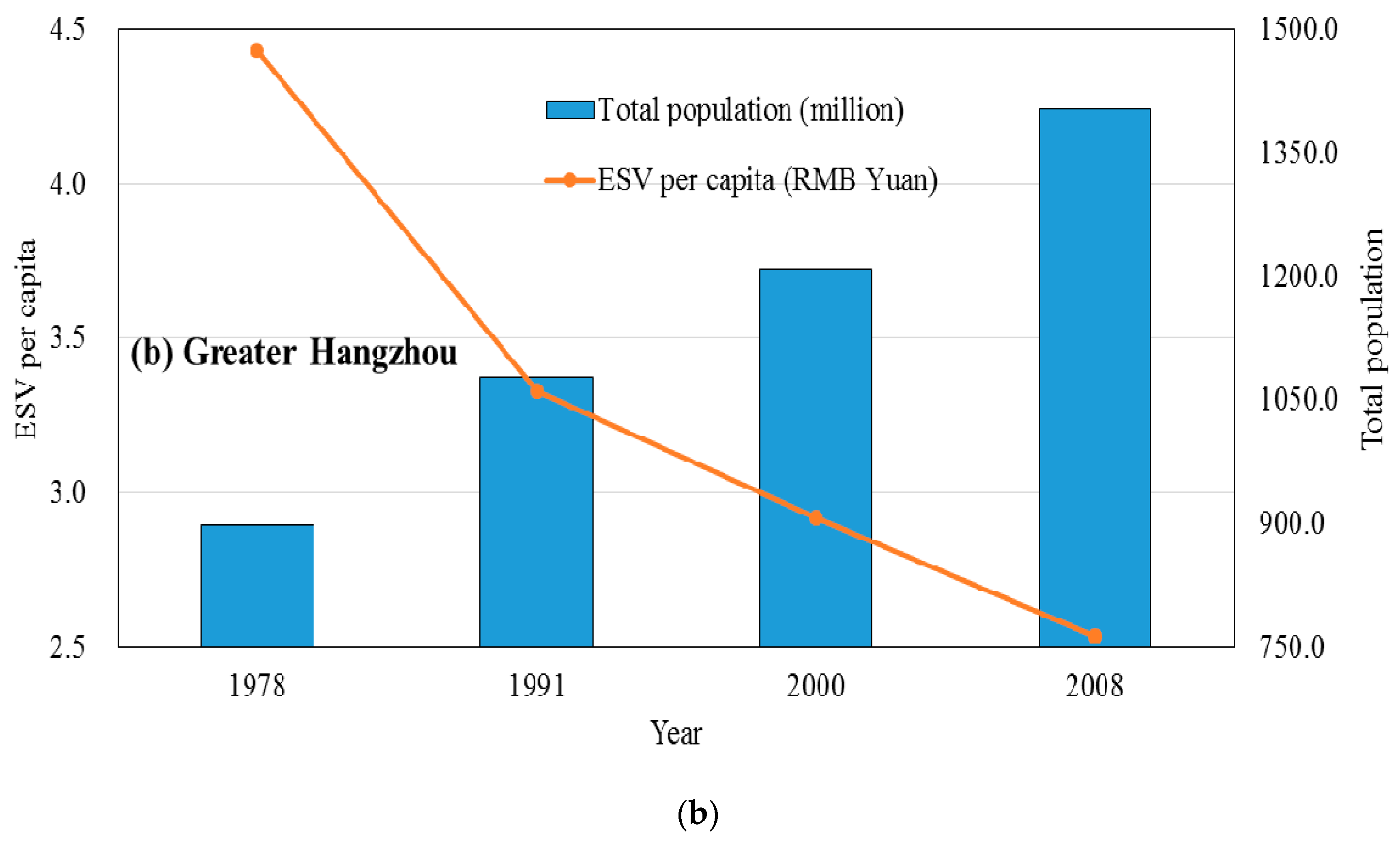
3.3. Variation in Spatiotemporal Pattern of ESV
3.4. Relationship between the Landscape Pattern and Allocation of Esv
4. Discussion
4.1. Revisiting the Cause-Effect Relationship between LULC Change, Landscape Fragmentation, and Ecosystems’ Functioning
4.2. Implications for Policies towards Sustainable Land Use and Ecosystem Management
4.3. Limitation of This Study
5. Conclusions
Acknowledgments
Author Contributions
Conflicts of Interest
Appendix A

| Study Area | On-Board Sensor | Path/Row | Acquisition Date (DD-MM-YY) | Resolution (m) |
|---|---|---|---|---|
| Greater Shanghai | MSS | 127/038, 127/039 | 4-8-1979 | 60 |
| TM | 118/038, 118/039 | 18-5-1987 | 30 | |
| TM | 118/038, 118/039 | 11-4-1997 | 30 | |
| Greater Hangzhou | TM | 118/038, 118/039 | 24-3-2008 | 30 |
| MSS | 128/039 | 5-7-1978 | 60 | |
| TM | 119/039 | 23-7-1991 | 30 | |
| ETM+ | 119/039 | 11-10-2000 | 30 | |
| ETM+ | 119/039 | 24-4-2008 | 30 |
| Land Cover Type | Description |
|---|---|
| Developed land | Visually detectable urban and rural settlements, commercial areas, transportation lines, and industrial parks. |
| Cropland | Paddy fields, fallow lands after harvest, and dry lands. |
| Forest | Natural and artificial woodlands. |
| Shrub | Wild scrubland and forest nurseries. |
| Water | Rivers, creeks, reservoirs, lakes, fishponds, and dikes. |
| Tidal land | Sandy flat periodically inundated by tides. |
| Bare land | Bare rocks, gravel pits, quarries, mines, permanently enclosed tidal land, and vacant land after clearing vegetation for urban development. |
| Formula | Description |
|---|---|
| where ni is counts of land cover patch (class) i, A is total area of all patches (m2). | |
| where Pi is percentage of patch type (class) i within the landscape, aij is area (m2) of patch ij, and A is area of all patches (m2). | |
| where aij is area (m2) of patch ij and A is total area of all patches (m2). | |
| where ei is class i’s total length of edge for given grids; min ei is class i’s minimum total length of edge. | |
| where Ai is class i’s area (m2), and Ni is number of class i. |
| Region | Buffers Distance (km) | Synopotical Description |
|---|---|---|
| Greater Shanghai | 0–6 | The city core of downtown Shanghai. |
| 6–12 | The newly in-filling urban area between the inner and outer rings. | |
| 12–21 | The urban finge with intensive settlements and industrial parks. | |
| 21–35 | The rapidly urbaning areas with intensive settlements, industrial parks, harbors, and airport | |
| >35 | The low-density developed rural areas with sparsely distributed towns and villages. Aside from some settlements and industrial parks, this zonal buffer is characterized with cropland and tidal land. | |
| Greater Hangzhou | 0–3 | The city core of downtown Hangzhou. |
| 3–6 | The newly in-filling urban area between the city core and neiboring towns. | |
| 6–15 | The rapidly urbanizing areas expanding eastward and southward between the city core and well-developed urban area of Xiaoshan district. | |
| 15–25 | The mixing middle-density and low-density developed rural areas with sparsely distributed towns and villages. Aside from the well-developed urban area of Yuhang district, this zonal buffer is characterzied with hilly terrain, cropland, and river network. | |
| >25 | The low-density developed rural areas with sparsely distributed towns and villages. This zonal buffer is characterzied with hilly and mountaineous terrain and tidal land. |
| Ecosystem Services Category | Ecosystem Service Functions | Land Use Category | |||||
|---|---|---|---|---|---|---|---|
| Forest | Cropland | Water | Shrub | Bare Land | Tidal Land | ||
| Regulating | Gas regulation | 3097.00 | 442.40 | 0.00 | 1769.70 | 0.00 | 0.00 |
| Climate regulation | 2389.10 | 787.50 | 407.00 | 1588.30 | 0.00 | 203.50 | |
| Supporting | Soil formation and retention | 3450.90 | 1291.90 | 8.80 | 2371.40 | 17.70 | 13.30 |
| Waste purification | 1159.20 | 1451.20 | 16086.60 | 1287.20 | 8.80 | 8047.70 | |
| Biodiversity protection | 2884.60 | 628.20 | 2203.30 | 1756.40 | 300.80 | 1252.10 | |
| Provisioning | Water supply | 2831.50 | 530.90 | 18,033.20 | 1681.20 | 26.50 | 9029.90 |
| Food production | 88.50 | 884.90 | 88.50 | 177.00 | 8.80 | 48.70 | |
| Raw material | 2300.60 | 88.50 | 8.80 | 1194.60 | 0.00 | 4.40 | |
| Cultural | Recreation and culture | 1132.60 | 8.80 | 3840.20 | 570.70 | 8.80 | 1924.50 |

References
- Dallimer, M.; Davies, Z.G.; Diaz-Porras, D.F.; Irvine, K.N.; Maltby, L.; Warren, P.H.; Armsworth, P.R.; Gaston, K.J. Historical influences on the current provision of multiple ecosystem services. Glob. Environ. Chang. 2015, 31, 307–317. [Google Scholar] [CrossRef]
- Elmhagen, B.; Eriksson, O.; Lindborg, R. Implications of climate and land-use change for landscape processes, biodiversity, ecosystem services, and governance. AMBIO 2015, 44, 1–5. [Google Scholar] [CrossRef] [PubMed]
- Grimm, N.B.; Foster, D.; Groffman, P.; Grove, J.M.; Hopkinson, C.S.; Nadelhoffer, K.J.; Pataki, D.E.; Peters, D.P.C. The changing landscape: Ecosystem responses to urbanization and pollution across climatic and societal gradients. Front. Ecol. Environ. 2008, 6, 264–272. [Google Scholar] [CrossRef]
- Larondelle, N.; Haase, D.; Kabisch, N. Mapping the diversity of regulating ecosystem services in European cities. Glob. Environ. Chang. 2014, 26, 119–129. [Google Scholar] [CrossRef]
- Millennium Ecosystem Assessment (MEA). Ecosystems and Human Wellbeing: Synthesis; Island Press: Washington, DC, USA, 2005. [Google Scholar]
- Munroe, D.K.; Croissant, C.; York, A.M. Land use policy and landscape fragmentation in an urbanizing region: Assessing the impact of zoning. Appl. Geogr. 2005, 25, 121–141. [Google Scholar] [CrossRef]
- Daily, G.C. (Ed.) Nature’s Services: Societal Dependence on Natural Ecosystems; Island Press: Washington, DC, USA, 1997.
- Estoque, R.C.; Murayama, Y. Landscape pattern and ecosystem service value changes: Implications for environmental sustainability planning for the rapidly urbanizing summer capital of the Philippines. Landsc. Urban Plan. 2013, 116, 60–72. [Google Scholar] [CrossRef]
- Shrestha, M.K.; York, A.M.; Boone, C.G.; Zhang, S. Land fragmentation due to rapid urbanization in the Phoenix Metropolitan Area: Analyzing the spatiotemporal patterns and drivers. Appl. Geogr. 2012, 32, 522–531. [Google Scholar] [CrossRef]
- Seto, K.C.; Fragkias, M. Quantifying spatiotemporal patterns of urban land-use change in four cities of China with time series landscape metrics. Landsc. Ecol. 2005, 20, 871–888. [Google Scholar] [CrossRef]
- Su, S.; Xiao, R.; Jiang, Z.; Zhang, Y. Characterizing landscape pattern and ecosystem service value changes for urbanization impacts at an eco-regional scale. Appl. Geogr. 2012, 34, 295–305. [Google Scholar] [CrossRef]
- Barral, M.P.; Maceira, N.O. Land-use planning based on ecosystem service assessment: A case study in the Southeast Pampas of Argentina. Agric. Ecosyst. Environ. 2012, 154, 34–43. [Google Scholar] [CrossRef]
- Goldstein, J.H.; Caldarone, J.; Duarte, T.K.; Ennaanay, D.; Hannahs, N.; Mendoza, G.; Polasky, S.; Wolny, S.; Daily, G. Integrating ecosystem-service tradeoffs into land-use decisions. Proc. Natl. Acad. Sci. USA 2012, 109, 7565–7570. [Google Scholar] [CrossRef] [PubMed]
- Kroll, F.; Müller, F.; Haase, D.; Fohrer, N. Rural-urban gradient analysis of ecosystem services supply and demand dynamics. Land Use Policy 2012, 29, 521–535. [Google Scholar] [CrossRef]
- United States Environmental Protection Agency’s Science Advisory Board (USEPA-SAB). Valuing the Protection of Ecological Systems and Services: A Report of the EPA Science Advisory Board (EPA-SAB-09-012). 2009. Available online: http://nepis.epa.gov/Exe/ZyPDF.cgi/P100DCSG.PDF?Dockey=P100DCSG.PDF (accessed on 5 June 2013). [Google Scholar]
- Frank, S.; Furst, C.; Koschke, L.; Makeschin, F. A contribution towards a transfer of the ecosystem service concept to landscape planning using landscape metrics. Ecol. Indic. 2012, 21, 30–38. [Google Scholar] [CrossRef]
- Grêt-Regamey, A.; Rabe, S.E.; Crespo, R.; Lautenbach, S.; Ryffel, A.; Schlup, B. On the importance of non-linear relationships between landscape patterns and the sustainable provision of ecosystem services. Landsc. Ecol. 2014, 29, 201–212. [Google Scholar] [CrossRef]
- Hogan, D.M.; Labiosa, W.; Pearlstine, L.; Hallac, D.; Strong, D.; Hearn, P.; Bernknopf, R. Estimating the cumulative ecological effect of local scale landscape changes in south Florida. Environ. Manag. 2012, 201, 502–515. [Google Scholar] [CrossRef] [PubMed]
- Sun, Y.-H.; Zong, Y.-G.; Ke, D.; Wang, B.; Wang, Y.-J. Application of spatial ecological value assessment for urban sprawl control: A case study in the central area of Xi’an, China. Mod. Urban Res. 2011, 5, 64–69. [Google Scholar]
- Syrbe, R.U.; Walz, U. Spatial indicators for the assessment of ecosystem services: Providing, benefiting and connecting areas and landscape metrics. Ecol. Indic. 2012, 21, 80–88. [Google Scholar] [CrossRef]
- Qi, Z.-F.; Ye, X.-Y.; Zhang, H.; Yu, Z.-L. Land fragmentation and variation of ecosystem services in the context of rapid urbanization: the case of Taizhou city, China. Stoch. Environ. Res. Risk Assess. 2014, 28, 843–855. [Google Scholar] [CrossRef]
- Zhang, M.; Wang, K.; Liu, H.; Zhang, C. Responses of ecosystem service values to landscape pattern change in typical Karst area of northwest Guangxi, China. Chin. Geogr. Sci. 2011, 21, 446–453. [Google Scholar] [CrossRef]
- Cai, Y.-B.; Zhang, H.; Pan, W.-B.; Chen, Y.-H.; Wang, X.-R. Land use pattern, socio-economic development, and assessment of their impacts on ecosystem service value: Study on natural wetlands distribution area (NWDA) in Fuzhou city, southeastern China. Environ. Monit. Assess. 2013, 185, 5111–5123. [Google Scholar] [CrossRef] [PubMed]
- Cheng, L.; Li, F.; Deng, H.-F. Dynamics of land use and its ecosystem services in China’s megacities. Acta Ecol. Sin. 2011, 31, 6194–6203. [Google Scholar]
- Liu, J.; Li, S.; Ouyang, Z.; Tam, C.; Chen, X. Ecological and socioeconomic effects of China’s policies for ecosystem services. Proc. Natl. Acad. Sci. USA 2008, 105, 9489–9494. [Google Scholar] [CrossRef] [PubMed]
- Long, H.; Liu, X.; Hou, X.; Li, T.; Li, Y. Effects of land use transitions due to rapid urbanization on ecosystem services: Implications for urban planning in the new developing area of China. Habitat Int. 2014, 44, 536–544. [Google Scholar] [CrossRef]
- Qiu, B.; Li, H.; Zhang, L. Vulnerability of ecosystem services provisioning to urbanization: A case of China. Ecol. Indic. 2015, 57, 505–513. [Google Scholar] [CrossRef]
- Song, W.; Deng, X. Effects of urbanization-Induced cultivated land loss on ecosystem services in the north China plain. Energies 2015, 8, 5678–5693. [Google Scholar] [CrossRef]
- Tan, J.; Zheng, Y.; Tang, X.; Guo, C.; Li, L.; Song, G.; Zhen, X.; Yuan, D.; Kalkstein, A.J.; Li, F. The urban heat island and its impact on heat waves and human health in Shanghai. Int. J. Biometeorol. 2010, 54, 75–84. [Google Scholar] [CrossRef] [PubMed]
- Wei, Y.-D.; Ye, X. Urbanization, urban land expansion and environmental change in China. Stoch. Environ. Res. Risk Assess. 2014, 28, 757–765. [Google Scholar] [CrossRef]
- Li, W.-M.; Li, B.-S. Research on the characteristic and the strategy of the development of new town in Hangzhou metropolitan area. J. Zhejiang Univ. 2005, 32, 108–114, 120. [Google Scholar]
- Shanghai Municipal Bureau of Statistics (SMBS). Shanghai Statistical Yearbook. 2013. Available online: http://www.stats-sh.gov.cn/data/toTjnj.xhtml?y=2013 (accessed on 30 July 2013). [Google Scholar]
- Hangzhou Municipal Bureau of Statistics (HMBS). Hangzhou Statistical Yearbook. 2013. Available online: http://www.hzstats.gov.cn/web/default.aspx (accessed on 23 October 2013). [Google Scholar]
- China National Bureau of Statistics (CNBS). National Data. Available online: http://data.stats.gov.cn/easyquery.htm?cn=C01 (accessed on 5 June 2014).
- Lin, Y.-M.; Bao, K. The impact of the scan lines corrector malfunction on Landsat-7 imagery data and the processing methods. Remote Sens. Inf. 2005, 2, 33–35. [Google Scholar]
- China National Committee of Agricultural Divisions. Technical Regulation of Investigation on Land Use Status; Surveying and Mapping Publishing House: Beijing, China, 1984. [Google Scholar]
- The Standard GIS-Based Altas of The Yangtze River Basin; Beijing Digital Space Technology Co., Ltd.: Beijing, China, 2015.
- Basic Geodatabase of Shanghai; Shanghai Institute for Geological Survey: Shanghai, China, 2001.
- The Standard GIS-Based Altas of Hangzhou Region; Hangzhou Land and Resources Administration and Hangzhou Institute for Planning and Designing: Hangzhou, China, 2005.
- Shalaby, A.; Tateishi, R. Remote sensing and GIS for mapping and monitoring land cover and land-use changes in the northwestern coastal zone of Egypt. Appl. Geogr. 2007, 27, 28–41. [Google Scholar] [CrossRef]
- Jassen, L.I.F.; Frans, J.M.; Wel, V.D. Accuracy assessment of satellite derived land-cover data: A review. Photogramm. Eng. Remote Sens. 1994, 60, 410–432. [Google Scholar]
- Singh, A. Digital change detection techniques using remotely sensed data. Int. J. Remote Sens. 1989, 10, 989–1003. [Google Scholar] [CrossRef]
- Zhang, H.; Zhou, L.-G.; Chen, M.-N.; Ma, W.-C. Land use dynamics of the fast-growing Shanghai Metropolis, China (1979–2008) and its implications for land use and urban planning policy. Sensors 2011, 11, 1794–1809. [Google Scholar] [CrossRef] [PubMed]
- Wu, K.-Y.; Zhang, H. Land use dynamics, expansion patterns of built-up land, and driving forces analysis of the fast-growing Hangzhou metropolitan area, eastern China (1978–2008). Appl. Geogr. 2012, 34, 137–145. [Google Scholar] [CrossRef]
- McGarigal, K.; Cushman, S.A.; Ene, E. FRAGSTATS v4: Spatial Pattern Analysis Program for Categorical and Continuous Maps. Computer Software Program Produced by the Authors at the University of Massachusetts, Amherst. Available online: http://www.umass.edu/landeco/research/fragstats/fragstats.html (accessed on 3 July 2014).
- Costanza, R.; d’Arge, R.; de Groot, R.; Farber, S.; Grasso, M.; Hannon, B.; Limburg, K.; Naeem, S.; O’Neill, R.V.; Paruelo, J.; et al. The value of the world’s ecosystem services and natural capital. Nature 1997, 387, 253–260. [Google Scholar] [CrossRef]
- Xie, G.; Lu, C.; Leng, Y.; Zheng, D.; Li, S. Ecological assets valuation of the Tibetan Plateau. J. Nat. Resour. 2003, 18, 189–196. [Google Scholar]
- Gao, H.-X. Applied Statistical Methods and SAS; Peking University Press: Beijing, China, 2001. [Google Scholar]
- Tang, Q.-Y.; Zhang, C.-X. Data Processing System (DPS) software with experimental design, statistical analysis and data mining developed for use in entomological research. Insect Sci. 2013, 20, 254–260. [Google Scholar] [CrossRef] [PubMed]
- Yue, W.-Z.; Liu, Y.; Fan, P.-L. Polycentric urban development: The case of Hangzhou. Environ. Plan. A 2010, 42, 563–577. [Google Scholar] [CrossRef]
- Wu, K.-Y.; Ye, X.-Y.; Qi, Z.-F.; Zhang, H. Impacts of land use/land cover change and socioeconomic development on regional ecosystem services: The case of fast-growing Hangzhou metropolitan area, China. Cities 2013, 31, 276–284. [Google Scholar] [CrossRef]
- Ollerton, J.; Erenler, H.; Edwards, M.; Crockett, R. Extinctions of aculeate pollinators in Britain and the role of large-scale agricultural changes. Science 2014, 346, 1360–1362. [Google Scholar] [CrossRef] [PubMed]
- Potts, S.G.; Vulliamy, B.; Roberts, S.; O’Toole, C.; Dafni, A.; Ne’eman, G.; Willmer, P. Role of nesting resources in organising diverse bee communities in a Mediterranean landscape. Ecol. Entomol. 2005, 30, 78–85. [Google Scholar] [CrossRef]
- Palma, A.D.; Kuhlmann, M.; Roberts, S.P.M.; Potts, S.G.; Börger, L.; Hudson, L.N.; Lysenko, I.; Newbold, T.; Purvis, A. Ecological traits affect the sensitivity of bees to land-use pressures in European agricultural landscapes. J. Appl. Ecol. 2015, 52, 1567–1577. [Google Scholar] [CrossRef] [Green Version]
- Leonard, P.B.; Sutherland, R.W.; Baldwin, R.F.; Fedak, D.A.; Carnes, R.G.; Montgomery, A.P. Landscape connectivity losses due to sea level rise and land use change. Anim. Conserv. 2016. [Google Scholar] [CrossRef]
- Concepción, E.D.; Götzenberger, L.; Nobis, M.P.; De Bello, F.; Obrist, M.K.; Moretti, M. Contrasting trait assembly patterns in plant and bird communities along environmental and human-induced land-use gradients. Ecography 2016. [Google Scholar] [CrossRef]
- Nuissl, H.; Haase, D.; Lanzendorf, M.; Wittmer, H. Environmental impact assessment of urban land use transitions—A context-sensitive approach. Land Use Policy 2009, 26, 414–424. [Google Scholar] [CrossRef]
- Rogan, J.; Wright, T.M.; Cardille, J.; Pearsall, H.; Ogneva-Himmelberger, Y.; Riemann, R.; Riitters, K.; Partington, K. Forest fragmentation in Massachusetts, USA: A town-level assessment using Morphological spatial pattern analysis and affinity propagation. GISci. Remote Sens. 2016, 53, 1–14. [Google Scholar] [CrossRef]
- Stürck, J.; Schulp, C.J.E.; Verburg, P.H. Spatio-temporal dynamics of regulating ecosystem services in Europe—The role of past and future land use change. Appl. Geogr. 2015, 63, 121–135. [Google Scholar] [CrossRef]
- Zank, B.; Bagstad, K.J.; Voigt, B.; Villa, F. Modeling the effects of urban expansion on natural capital stocks and ecosystem service flows: A case study in the Puget Sound, Washington, USA. Landsc. Urban Plan. 2016, 149, 31–42. [Google Scholar] [CrossRef]
- Deng, J.S.; Qi, L.F.; Wang, K.; Yang, H.; Shi, Y.Y. An integrated analysis of urbanization-triggered cropland loss trajectory and implications for sustainable land management. Cities 2011, 28, 127–137. [Google Scholar] [CrossRef]
- Liu, Y.S.; Wang, J.Y.; Long, H.L. Analysis of arable land loss and its impact on rural sustainability in Southern Jiangsu Province of China. J. Environ. Manag. 2010, 91, 646–653. [Google Scholar] [CrossRef] [PubMed]
- Zhong, T.-Y.; Huang, X.-J.; Zhang, X.-Y.; Wang, K. Temporal and spatial variability of agricultural land loss in relation to policy and accessibility in a low hilly region of southeast China. Land Use Policy 2011, 28, 762–769. [Google Scholar] [CrossRef]


| LULC Type | Developed Land | Cropland | Forest | Water | Tidal Land | Bare Land | ||||||
|---|---|---|---|---|---|---|---|---|---|---|---|---|
| R (%) | C (%) | R (%) | C (%) | R (%) | C (%) | R (%) | C (%) | R (%) | C (%) | R (%) | C (%) | |
| Developed land | 75.00–87.10 | 62.50–71.15 | 0 | 0 | 0 | 0 | 0–7.32 | 0–7.67 | 3.57–5.56 | 4.55–6.67 | 14.63–25.00 | 15.79–22.92 |
| Cropland | 0 | 0 | 62.5–80.49 | 76.92–100.00 | 10.20–35.42 | 16.67–32.69 | 0 | 0 | 0–2.44 | 0–2.70 | 0–10.20 | 0–10.42 |
| Forest | 0 | 0 | 0–20.45 | 0–23.08 | 76.09–100.00 | 67.31–83.33 | 0 | 0 | 0–4.35 | 0–4.55 | 0 | 0 |
| Water | 0–2.33 | 0–2.86 | 0 | 0 | 0 | 0 | 77.78–86.05 | 84.85–100.00 | 11.63–23.91 | 11.36–29.73 | 0 | 0 |
| Tidal land | 2.77–8.00 | 2.44–4.65 | 0 | 0 | 0–4.65 | 0–6.67 | 0–11.63 | 0–15.55 | 67.44–80.00 | 54.05–75.00 | 8.11–12.00 | 5.77–13.16 |
| Bare land | 2.44–13.89 | 2.13–12.20 | 0 | 0 | 0 | 0 | 0 | 0 | 3.23–12.5 | 2.27–11.11 | 75.00–90.24 | 62.50–71.15 |
| UA (%) | 76.88–82.81 | |||||||||||
| PA (%) | 76.93–83.48 | |||||||||||
| OA (%) | 76.40–84.20 | |||||||||||
| Kappa statistic | 0.72–0.79 | |||||||||||
| LULC Type | Developed Land | Cropland | Forest | Shrub | Water | Tidal Land | Bare Land | |||||||
|---|---|---|---|---|---|---|---|---|---|---|---|---|---|---|
| R (%) | C (%) | R (%) | C (%) | R (%) | C (%) | R (%) | C (%) | R (%) | C (%) | R (%) | C (%) | R (%) | C (%) | |
| Developed land | 68.90–84.80 | 83.09–92.01 | 0–1.71 | 0.76–4.29 | 0–1.78 | 0–2.33 | 0–0.67 | 0.65–4.24 | 0–4.11 | 0–2.89 | 0–5.15 | 0–8.21 | 0–4.90 | 0–5.32 |
| Cropland | 1.75–11.59 | 0–4.66 | 69.90–95.81 | 83.75–92.31 | 2.79–13.10 | 3.61–11.44 | 0–11.26 | 0–9.71 | 0.56–9.58 | 0.32–2.35 | 2.11–13.16 | 0–3.17 | 0–6.80 | 0–23.61 |
| Forest | 0–4.68 | 0–2.40 | 1.25–5.97 | 1.22–4.29 | 75.86–96.17 | 80.47–92.88 | 0–3.36 | 0–7.79 | 0–1.58 | 0–2.31 | 0–1.58 | 0 | 0–0.91 | 0–0.69 |
| Shrub | 0.58–9.76 | 0–0.65 | 0–5.24 | 0–3.84 | 0–10.34 | 0–4.03 | 81.46–98.34 | 79.87–96.74 | 0–3.42 | 0–1.54 | 0–3.68 | 0–6.72 | 0–5.88 | 0–0.70 |
| Water | 0–5.49 | 0–9.56 | 0.19–1.73 | 0.23–5.95 | 0–1.33 | 0–3.25 | 0–1.32 | 0–3.25 | 81.57–96.05 | 73.08–96.38 | 0–30.00 | 1.14–9.51 | 0–2.94 | 0–4.90 |
| Tidal land | 0–6.43 | 0–4.41 | 0–0.76 | 0.77–5.73 | 0 | 0–1.49 | 0–5.96 | 0–4.00 | 0.49–10.57 | 0–21.79 | 49.12–96.32 | 74.63–95.43 | 0–2.90 | 0–31.47 |
| Bare land | 0–10.55 | 0–3.27 | 0–9.43 | 0–3.44 | 0–1.63 | 0–1.49 | 0–1.34 | 0–1.63 | 0–1.72 | 0–0.64 | 0–13.24 | 0–4.48 | 83.33–100.00 | 59.44–100.00 |
| UA (%) | 83.19–88.31 | |||||||||||||
| PA (%) | 82.54–86.99 | |||||||||||||
| OA (%) | 80.70–88.56 | |||||||||||||
| Kappa statistic | 0.78–0.85 | |||||||||||||
| Ecosystem Service Category | Greater Shanghai | Greater Hangzhou | ||||||
|---|---|---|---|---|---|---|---|---|
| 1979 | 1987 | 1997 | 2008 | 1978 | 1991 | 2000 | 2008 | |
| Regulating | 1101.19 | 916.58 | 844.39 | 747.97 | 780.93 | 658.26 | 616.03 | 563.7 |
| Supporting | 9409.11 | 8514.57 | 8548.44 | 7725.88 | 1894.61 | 1620.96 | 1527.04 | 1442.6 |
| Provisioning | 8264.66 | 7437.53 | 7489.05 | 6844.91 | 1343.87 | 1111.41 | 1055.24 | 1043.8 |
| Cultural | 1595.93 | 1419.73 | 1425.49 | 1323.73 | 246.69 | 189.13 | 180.86 | 190.31 |
| Sum | 21,966.82 | 19,708.14 | 19,732.86 | 17,966.22 | 4512.79 | 3768.89 | 3560.03 | 3430.7 |
| Zonal Buffer | Year | Stage Change Rate | ||||||
|---|---|---|---|---|---|---|---|---|
| 1979 | 1987 | 1997 | 2008 | 1979–1987 | 1987–1997 | 1997–2008 | 1978–2008 | |
| 0–6 km | 59.84 | 39.87 | 35.25 | 41.05 | −33.36% | −11.61% | 16.48% | −31.39% |
| 6–12 km | 236.82 | 164.71 | 98.65 | 109.82 | −30.45% | −40.11% | 11.32% | −53.63% |
| 12–21 km | 780.60 | 650.36 | 660.73 | 484.66 | −16.69% | 1.60% | −26.65% | −37.91% |
| 21–35 km | 3748.93 | 3522.41 | 3682.43 | 3311.89 | −6.04% | 4.54% | −10.06% | −11.66% |
| >35 km | 15,544.69 | 13,911.03 | 13,830.31 | 12,695.06 | −10.51% | −0.58% | −8.21% | −18.33% |
| Zonal Buffer | Year | Stage Change Rate | ||||||
|---|---|---|---|---|---|---|---|---|
| 1978 | 1991 | 2000 | 2008 | 1979–1991 | 1991–2000 | 2000–2008 | 1978–2008 | |
| 0–3 km | 16.49 | 6.79 | 8.93 | 13.90 | −58.82% | 31.52% | 55.66% | −15.71% |
| 3–6 km | 92.68 | 62.35 | 55.42 | 67.41 | −32.73% | −11.11% | 21.63% | −27.27% |
| 6–15 km | 746.42 | 671.23 | 585.21 | 524.87 | −10.07% | −12.82% | −10.31% | −29.68% |
| 15–25 km | 1287.31 | 1191.25 | 1115.90 | 989.62 | −7.46% | −6.33% | −11.32% | −23.12% |
| >25 km | 2123.18 | 1931.19 | 1965.73 | 1912.66 | −9.04% | 1.79% | −2.70% | −9.92% |
| Multi-Linear Regression Model | R2 | |
|---|---|---|
| Ln ESVSH = 6.142 − 0.042 LPID + 0.001MPSC + 0.001 MPSF + 0.007 PLANDW+ 0.002 LSIT | 0.993 ** | (3) |
| Ln ESVHZ = 2.355 − 0.011 LPID + 0.013 LSIC + 0.036 PLANDF − 0.002 MPSB + 0.178 MPST | 0.990 ** | (4) |
© 2016 by the authors; licensee MDPI, Basel, Switzerland. This article is an open access article distributed under the terms and conditions of the Creative Commons Attribution (CC-BY) license (http://creativecommons.org/licenses/by/4.0/).
Share and Cite
Cai, Y.-B.; Li, H.-M.; Ye, X.-Y.; Zhang, H. Analyzing Three-Decadal Patterns of Land Use/Land Cover Change and Regional Ecosystem Services at the Landscape Level: Case Study of Two Coastal Metropolitan Regions, Eastern China. Sustainability 2016, 8, 773. https://0-doi-org.brum.beds.ac.uk/10.3390/su8080773
Cai Y-B, Li H-M, Ye X-Y, Zhang H. Analyzing Three-Decadal Patterns of Land Use/Land Cover Change and Regional Ecosystem Services at the Landscape Level: Case Study of Two Coastal Metropolitan Regions, Eastern China. Sustainability. 2016; 8(8):773. https://0-doi-org.brum.beds.ac.uk/10.3390/su8080773
Chicago/Turabian StyleCai, Yuan-Bin, Hui-Min Li, Xin-Yue Ye, and Hao Zhang. 2016. "Analyzing Three-Decadal Patterns of Land Use/Land Cover Change and Regional Ecosystem Services at the Landscape Level: Case Study of Two Coastal Metropolitan Regions, Eastern China" Sustainability 8, no. 8: 773. https://0-doi-org.brum.beds.ac.uk/10.3390/su8080773