Article

Variability of Temperature and Its Impact on Reference Evapotranspiration: The Test Case of the Apulia Region (Southern Italy)

by
Abderraouf Elferchichi
1,
Giuseppina A. Giorgio
2,*,
Nicola Lamaddalena
3,
Maria Ragosta
2 and
Vito Telesca
2,4
1
Regional Commissionership of Agricultural Development, 4200 Kebili, Tunisia
2
School of Engineering, University of Basilicata, 85100 Potenza, Italy
3
Mediterranean Agronomic Institute of Bari, CIHEAM Bari, Land and Water Division, 70010 Valenzano, Italy
4
CMCC—Euro-Mediterranean Center on Climate Change, 73100 Lecce, Italy
*
Author to whom correspondence should be addressed.
Sustainability 2017, 9(12), 2337; https://0-doi-org.brum.beds.ac.uk/10.3390/su9122337
Submission received: 21 October 2017 / Revised: 1 December 2017 / Accepted: 12 December 2017 / Published: 15 December 2017

Abstract

:
The present study provides an assessment of the climate variability at a subnational scale, focusing on the case of the Apulia region, in Southeastern Italy. The variables considered for the purpose of a trend analysis were the minimum, maximum, and mean temperatures, and reference evapotranspiration. These are very important in an urban–rural planning context. The study was based on 38 monitoring stations and consisted in the application of the nonparametric Mann–Kendall test and a progressive trend analysis, both used to detect the changes. The 1950–2003 period was investigated on seasonal and annual scales. The results generally showed a warming process and an acceleration of the atmospheric evaporative demand which took place especially since the mid-1970s. The latter had a significant positive trend, while the period before the break point of the 70s had a cooling effect. Finally, the warming effect was more pronounced for minimum temperatures.

Graphical Abstract

1. Introduction

The climate system and their associated variables are very complex. In the last three decades, many studies have addressed the issue of climate evolution under anthropic pressure [1]. An increase of the annual mean global temperature and changes of other climate parameters have been observed in the last century [2,3,4,5]. In fact, many papers particularly concern global climate modelling and the recent warming due to human activity. In particular, the fifth Assessment Report of the Intergovernmental Panel on Climate Change ascribed the dominant cause of the recent warming to human influence [6,7]. The overall effect of human activities on climate since the start of the industrial era has had a warming influence [8] especially in urban areas, leading to the Urban Heat Island (UHI) phenomena [9,10,11]. However, warming is variable in different seasons or in different locations. Instrumental observations show that temperatures at the surface have risen globally, with important regional variations [12]. Since 1880, average temperatures have increased by 0.8 °C around the world, much of this in recent decades. The 20th century’s last two decades were the hottest in 400 years. The United Nations’ IPCC reports that 11 of the past 12 years are among the warmest dozen since 1850. In addition, minimum temperatures increased about twice as fast as maximum temperatures over global land areas since 1950, resulting in a broad decline in the diurnal temperature range [13,14,15].
Italy is located in the middle of the Mediterranean region and has been identified as one of the most sensitive areas to greenhouse gas (GHG)-induced global warming [16,17]. The local climate change is very different in various areas of the country because of the high variety of the topographic and geographical features. In Southern Italy, a temperature increase seems to prevail, especially since about 1980 [18].
In recent years, many studies were carried out concerning the estimation of actual and reference evapotranspiration based on remote sensing analysis and in situ measurements. Potential evapotranspiration is an important parameter for different applications in hydrological modelling, irrigation, and environmental studies. Several methods for the estimation of potential evapotranspiration are available in the literature, based on radiation or temperatures. Tegos et al. (2015) presented a parametric method which implements spatially varying parameters calibrated on the basis of potential evapotranspiration data [18,19,20,21,22,23,24]. Recently, landscape planning has been related to climate change; in particular, the knowledge of variables, especially temperatures and evapotranspiration, plays an important role in urban and rural planning policies [25,26,27,28,29]. Development plans should not be rendered meaningless by a significant change in weather and climate behavior. Therefore, indications of possible climatic variability and of increasingly frequent and serious extreme events in the context of global climate change are necessary within the framework of agrometeorological services, in addition to the application of other agrometeorological information. In fact, detailed observations and monitoring, as well as the real-time dissemination of meteorological information, quantification by remote sensing (radar and satellites), and derived indices and operational services are important for tactical agrometeorological decisions in the short-term planning of agricultural operations at different growth stages [30,31,32,33,34,35].
This study analyzed the weather climatic events in two temporal scales (1950–2003 and 1974–2003) in order to define a detailed climatic overview and estimate potential variations at a local scale. In particular, the aim of this study was to investigate the spatial–temporal variability of temperature and to evaluate its impact on reference evapotranspiration in the Apulia region (Southern Italy).
Here, two time directions were considered: a direct progressive trend analysis and an inverse progressive trend analysis.
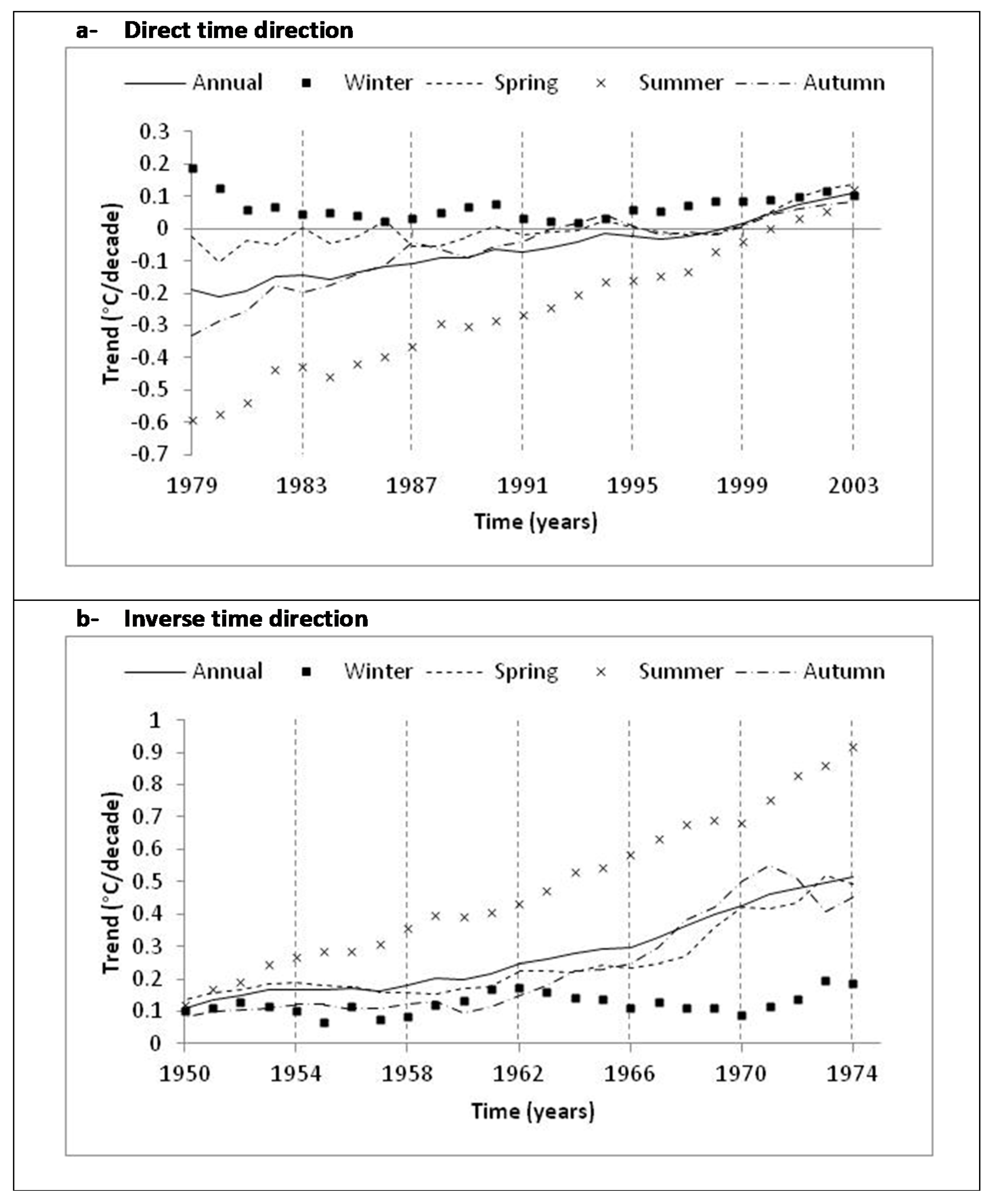
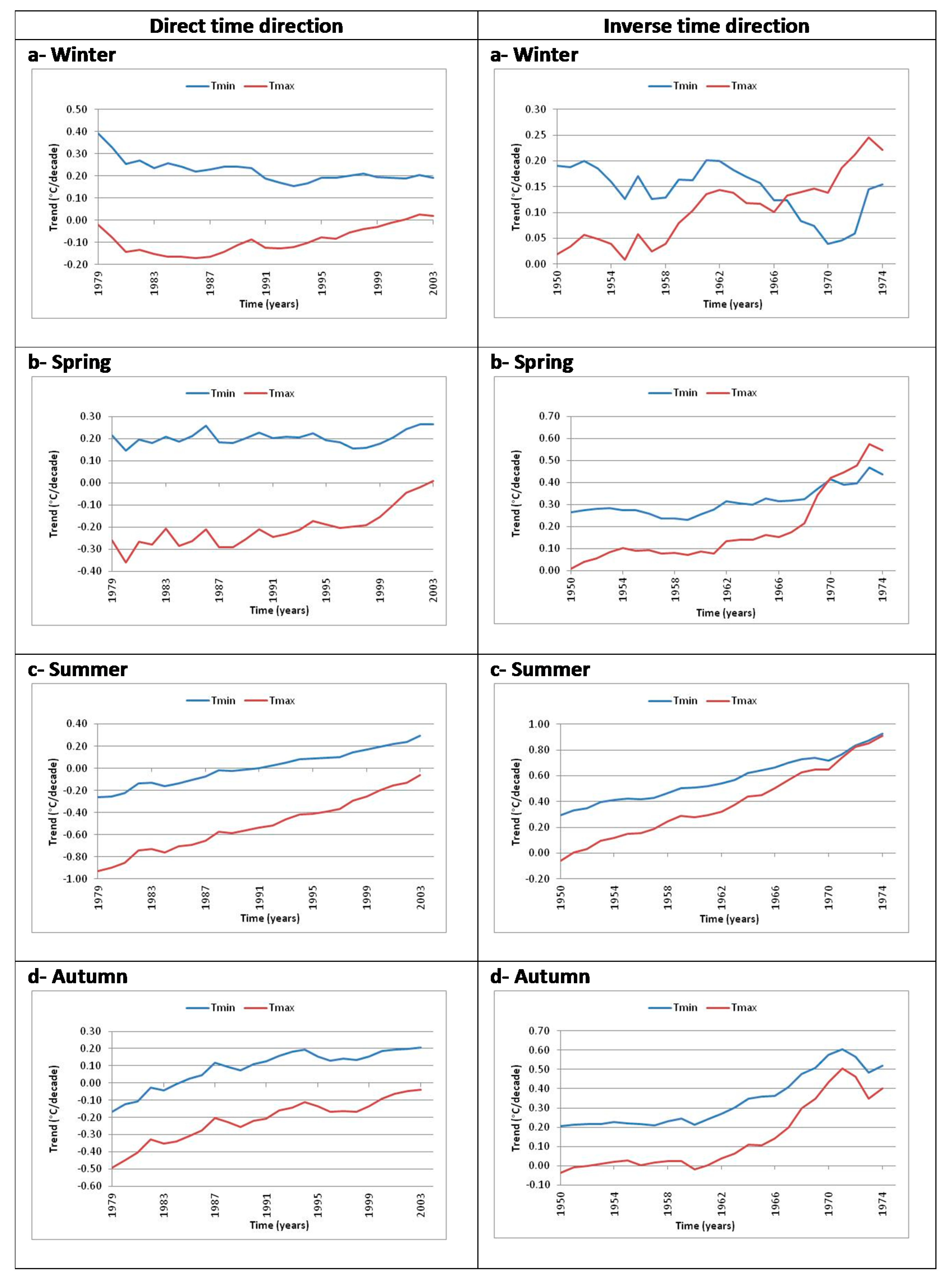
  • In the “direct time direction” case, 1950–1979 represents a common period for a 25 subseries (selected period). The first subseries is 1950–1979, the second one is 1950–1980. By iteration, the last subseries is 1950–2003.
  • In the “inverse time direction” case, 1974–2003 represents a common period for a 25 subseries. The first subseries is 1974–2003, the second one is 1973–2003. By iteration, the last subseries is 1950–2003.

2. Study Area and Data

This study analyzed minimum and maximum monthly temperatures from 1950 to 2003 in 38 of the 71 monitoring stations, managed by the hydrographic office of the Apulia region.
The Apulia region belongs to southeastern Italy and it is located approximately between latitudes 39.75°N and 41.9°N and longitudes 14.9°E and 18.5°E. It is bordered by the Adriatic Sea on the east, the Jonian Sea on the southeast, and the Strait of Òtranto and Gulf of Taranto on the south. The region comprises 19,345 km2, and its population is about four million. Based on the morphological, geological, and climatic aspects, the Apulia region is subdivided into eight landscapes: Appennino Dauno, Rilievi del Gargano, Tavoliere delle Puglie, Fossa Bradanica, Murge, Grandi valli terrazzate, Penisola salentina, and Arco ionico tarantino. The Apulia region is characterized by a typically Mediterranean climate with mild winters and hot summers that are generally long and dry [36].
In Figure 1, the density and the distribution of the monitoring stations are shown. In this case study, only the stations with less than 15% of missing data were considered (38 stations).
In this study, the investigated parameters were: maximum temperature (Tmax), minimum temperature (Tmin), mean temperature (Tm), and reference evapotranspiration (ETref). ETref is the standardized reference for clipped grass (ETo) or alfalfa (ETr) surfaces [37]. Various methods are available for ETref. These methods range from the most complex energy balance equations requiring detailed climatological data (e.g., Penman–Monteith) [38] to simpler equations requiring limited data (e.g., Blaney–Criddle, Hargreaves–Samani) [24,39,40].
In order to estimate the impact of temperature variability on reference evapotranspiration ETref, the Blaney–Criddle procedure was used. The Blaney–Criddle procedure is well known and has been used extensively in other scientific studies [40,41,42,43]. The usual form of the Blaney–Criddle equation converted to metric units is written as:
ETref = p (0.46 Tm + 8.13)
where ETref is the reference crop of clipped grass evapotranspiration (in mm/day), Tm is the average temperature over the period (in °C), and p is the mean daily percentage of annual daytime hours.

3. Methods

For trend detection, the nonparametric Mann–Kendall test [44,45] and the linear regression model (least-squares linear fitting models) for the examination of trends significance were used. The coefficient of determination (R2) from the least-squares linear fitting model (known as the linear regression model) was used to evaluate the trend linearity of the time series, while the coefficient value of the same model represents the trend magnitude, given in term of units per decade. In order to highlight temperature seasonality, the analysis was carried out considering the entire period (1950–2003) and the last three decades (1974–1983; 1984–1993; 1994–2003).
The Mann–Kendall test for trend detection is a simple and robust method, widely used in hydrometeorological time series such as precipitation, temperature, and stream flow [46,47,48,49,50,51,52]. The Mann–Kendall test determines whether the observations in the data tend to increase or decrease with time (this test is also referred to as Kendall’s tau when the x-axis is time). The null hypothesis for this test states that all observations are independent. On the other hand, the alternative hypothesis assumes that a monotonic trend, positive or negative, exists in the time series. In this analysis, the Mann–Kendall test is applied to detect if a trend in the temperature time series is statistically significant at 0.05 (95%), 0.01 (99%), and 0.1 (90%) significant levels (confidence intervals) for a two-sided probability. The Mann–Kendall test, however, does not provide an estimate of the magnitude of the trend. Moreover, the Mann–Kendall test is widely used because it is a distribution-free test. It has the advantage of not making hypotheses on the distribution function of the data. In this way, the results of the test are less influenced by the occurrence of outliers. It is therefore more suitable for detecting trends in hydrological time series, which are usually skewed and may be contaminated with outliers [48,53].
Climate change can be detected by the Kendall coefficient t (Mann test), and when a time series shows a significant trend, the period from which the trend is demonstrated can be obtained effectively by this test. In a time series, for each element yi, the number ni of elements yj preceding it (i > j) is calculated such that yi > yj. The test statistic t is then given by:
t = i n i
and is distributed very nearly as a Gaussian normal distribution with an expected value of E(t) = n(n − 1)/4 and a variance of var t = n(n − 1)(2n + 5)/72. A trend can be seen for high values of | u ( t ) | , where
u ( t ) = [ t E ( t ) ] / v a r   t
This principle can be usefully extended to the backward series, and u i = u ( t i ) can be obtained. The intersection of the u(t) and u′(t) curves denotes approximately the beginning of the trend. This is called the sequential version of the Mann–Kendall test [54,55,56,57,58].
For each confidence level, four significant classes were identified:
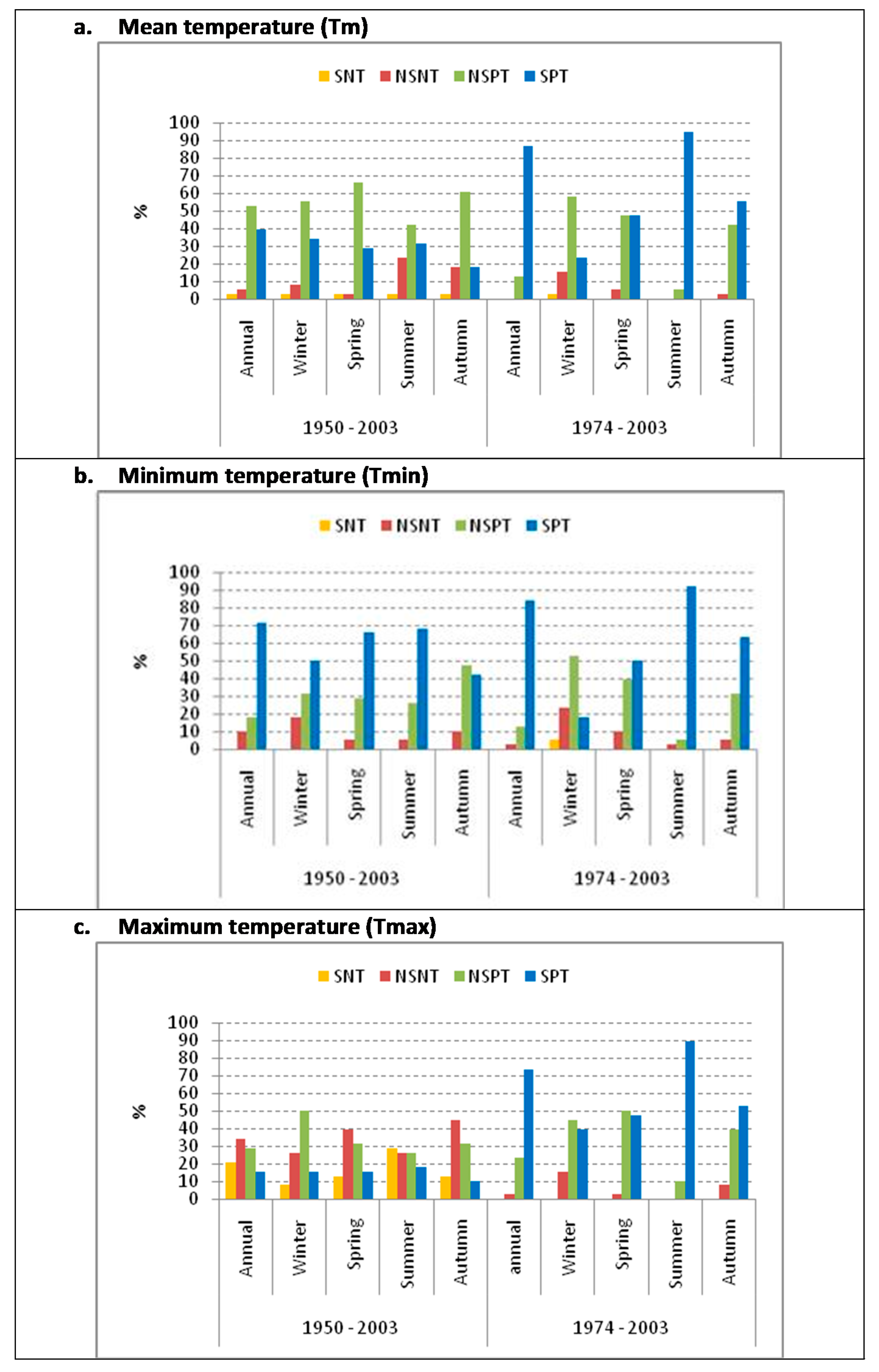
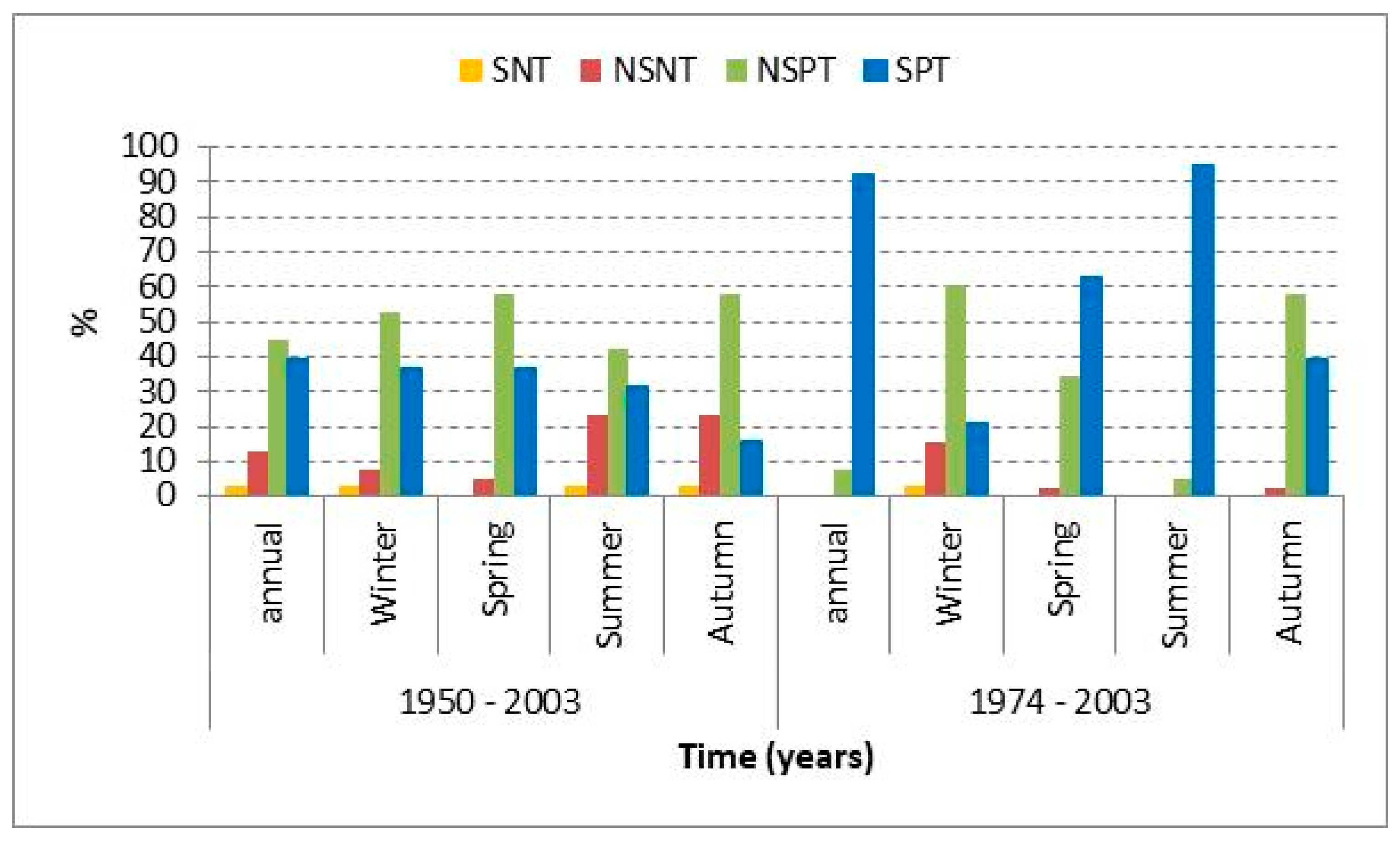
  • NSNT: Non-Significant Negative Trend;
  • SNT: Significant Negative Trend;
  • NSPT: Non-Significant Positive Trend;
  • SPT: Significant Positive Trend.
A progressive trend analysis was performed in order to highlight variations inside the overall period [58,59,60].
Annual and seasonal time scales were used for temperature analysis. In addition, two periods were analyzed: the entire period 1950–2003 and the last three decades (1974–1983; 1984–1993; 1994–2003). A progressive trend analysis was performed also in order to put in evidence the dependence of the trend on the selected period (30 years minimum) which is called a subseries. Furthermore, two directions were considered: direct progressive trend analysis and inverse progressive trend analysis. For the first direction, the subseries of 1979 which refers to 1950–1979 was considered the first one. The next subseries was 1980 (period 1950–1980). Therefore, the last subseries was 2003 and it referred to the entire period 1950–2003. For the second direction, 1974–2003 was considered a common period represented by 1974 and it was the first subseries to be analyzed. By going back in time, 1973 was the second subseries analyzed which referred to 1973–2003, and the last subseries was 1950–2003, represented by 1950. Consequently, the first set of subseries put in evidence the impact of the last 25 years of the covered period on the trend, whereas the second set analyzed the influence of the first 25 years of the covered period. The impact was studied, in fact, year by year.

4. Results and Discussion

The seasonal scale in the second half of the 20th century (1950–2003) was analyzed. A positive trend in the annual scale for mean temperatures in the overall period was shown in 92% of the examined stations. The maximum percentage of stations that showed a negative trend was observed in summer (26.3%). Considering a confidence level of 95%, the results showed the predominance of the NSPT class and a quite high percentage of the SPT class, as shown in Figure 2a. Only 2.6% of the stations showed an SNT class.
Similar results at 1% significance level showed a zero percentage of the SNT class on a seasonal scale and again 2.6% on the annual scale.
Regarding the last three decades of the entire period, all stations (100%) showed an evident warming process in terms of Tm. Furthermore, they were dominated by the SPT class. The percentages remained high for most of the stations even at 1% significance level, especially in summer (about 87% of the stations).
Regarding the entire period, the warming process was more related to minimum temperatures in the study area (Figure 2b,c), while maximum temperature trends were not evident (almost equal percentages of the positive and negative trends). However, during the last three decades, both Tmax and Tmin significantly participated in the warming.
The average trends obtained by a linear regression analysis in the study area are summarized in Table 1 (°C/decade). In addition, it was possible to show the dominance of the SPT class during the last three decades in the seasonal trend magnitudes, but less in the winter season. In particular, in terms of Tm, the summer season showed an average trend of 0.91°C/decade. These trends were much higher than the trend magnitudes of the overall period.
Therefore, it is possible to note again the effect of climate on Tmin: on the overall period, all average trends were significant at a 99% confidence level; on the contrary, trend magnitudes of Tmax were not significant and were close to zero °C/decade.
In order to detect any eventual spatial pattern of the changes in the study area, the Geographic Information System (GIS) was used. A GIS is a computer tool permitting to represent and to analyze all geographical objects as well as all events that produce them. A GIS permits the storage of the information concerning the world under the shape of thematic layers bound to one another by geography [61].
In particular, the interpolation scheme using the leave-one-out cross-validation method with the measured temperature data in 38 meteorological stations was used. The interpolation scheme used the inverse distance weighting (IDW). The IDW method is one of the most frequently used deterministic models in spatial interpolation because it has been implemented in many GIS packages. The general premise of this method is that the attribute values of any given pair of points are related to each other, but their similarity is inversely related to the distance between the two locations [62].
In Figure 3, the spatial interpolation of the Tm trend magnitude on a seasonal scale is shown. In addition to the evident warming, a clear spatial pattern was observed during the last three decades.
The temperatures illustrated a nonlinear trend for the overall period and in all stations, as shown in Table 2 by the average determination coefficient (R2) of the linear regression model, whereas, in the last three decades, R2 was quite high especially for the summer season in the 1974–2003 period.
In accordance to the nonlinear trend, the significance and magnitude trends, which depend on the selected period of analysis, were shown.
In order to effectively highlight the trend dependency on the selected period, a progressive trend analysis was performed on the average of the time series. The results are shown in Figure 4 and Figure 5 which demonstrate that the observed positive trend of Tm in the study area (Figure 4a) was determined by the last five years (1998 to 2003). Furthermore, warming was generally due to Tmin (Figure 5). In fact, the Tmin trend was generally positive, with some exception in the summer and autumn seasons (Figure 5c,d).
For direct time direction (Figure 4a), the subseries of 1979, which refers to 1950–1979, was considered as the first one. The next subseries was 1980, referring to the 1950–1980 period. Therefore, the last subseries was 2003 and it referred to the 1950–2003 period.
For inverse time direction (Figure 4b), the subseries of 1974, which referred to 1974–2003, was considered as the first one. The next subseries was 1973, referring to the 1973–2003 period. Therefore, the last subseries was 1950 and it referred to the 1950–2003 period.
Moreover, in terms of trend significance, the reference evapotranspiration followed the same behavior and direction in a similar way as the mean temperature; this was due to the high correlation between them. Indeed, as shown in Figure 6, a significant acceleration of the atmospheric evaporative demand was observed especially during the last three decades, in particular in the summer and spring seasons. A particular relevance of the significant positive trend of ETref was observed for most of the stations (about 87%) in the summer season, even at a 99% confidence level (Figure 6).
The average magnitude and significance trends are presented in Table 3. These trends, expressed in mm/decade, must be multiplied by 10 to get the equivalent trend in m3/ha. In terms of trend significance, the reference evapotranspiration followed the same behavior and direction as the mean temperature, with a much higher trend than the trend magnitudes of the entire period at the annual time scale in the summer season during the last three decades.
The reference evapotranspiration trend was not linear and, therefore, depended on the selected period of analysis. In fact, as shown in Figure 7, the solid black lines represent the five-year moving average curves of the series. The results were presented in terms of ETref anomalies with respect to the 1961–1990 base period.
The impact of the warming process in terms of magnitude of ETref was not important in the overall period. However, the impact was more evident during the last three decades, especially in the summer season and on the annual scale. Considering the similarity between the Tm and ETref behaviors, the period between 1950 and 1980 had a cooling effect especially on the annual scale (Figure 7e) in the summer season (Figure 7c).

5. Conclusions

In accordance to the results obtained by several studies [14,18,60], the present study confirms that the changes in climate were more pronounced in the patterns of the minimum temperature. Furthermore, since the 1970s, a break period has occurred at an increasing rate. Nevertheless, trend magnitudes in the study area during the last three decades were approximately double the global trend magnitude found by Trenberth et al. [14] in the 1979–2004 period.
The results showed a seasonal warming that was observed starting from the mid-1970s, which was significant at least at a 90% confidence level. In particular, the trend in summer was highly significant (<1%) with a trend magnitude of 0.91 ± 0.08 °C/decade. The average annual trend was 0.52 ± 0.07 °C/decade; on the contrary, the period before the end of 1980 showed a cooling effect.
Trend magnitude and significance strongly depended on the selected period as demonstrated by the progressive trend analysis. Considering the entire period, the last five years (1998 to 2003) showed a major significance in the trend, and the negative trend was presented for all seasons on the annual scale. Thus, trends were highly influenced by the last five years of the covered period.
It is possible to admit that the evident warming process, in terms of average temperatures, shown in all stations for the last three decades was different compared with the entire period, where there were no evident climate changes. This could be due to the limited data available in the three analyzed decades in the 1950–2003 period.
The impact on reference evapotranspiration was evident if the last three decades were considered. In particular, it was highly significant (<1%) in the summer (10.8 ± 1.0 mm/decade) and on the annual scale (18.6 ± 2.2 mm/decade).
The next studies will focus on an extension of the analyzed time period in order to determine whether the tendencies identified in this paper were confirmed in the successive decade.

Supplementary Files

Supplementary File 1

Acknowledgments

This research was carried out in the framework of the project ‘Smart Basilicata’ which was approved by the Italian Ministry of Education, University, and Research (MIUR D.M. No. 2078/2015) and was funded by the Cohesion Fund 2007–2013 of the Basilicata Regional authority (Grant No. 6386-3/2016).

Author Contributions

All authors contributed equally to this work in all its phases: conception and design of the project, its execution, analysis and interpretation of data. All authors read and approved the final manuscript for submission.

Conflicts of Interest

The authors declare no conflict of interest.

References

  1. Déqué, M.; Calmanti, S.; Christensen, O.B.; Aquila, A.D.; Maule, C.F.; Haensler, A.; Nikulin, G.; Teichmann, C. A multi-model climate response over tropical Africa at +2° C. Clim. Serv. 2016, 7, 87–95. [Google Scholar] [CrossRef]
  2. Cioffi, F.; Conticello, F.; Lall, U.; Marotta, L.; Telesca, V. Large scale climate and rainfall seasonality in a Mediterranean Area: Insights from a non-homogeneous Markov model applied to the Agro-Pontino plain. Hydrol. Process. 2017, 31, 668–686. [Google Scholar] [CrossRef]
  3. Giorgi, F.; Lionello, P. Climate change projections for the Mediterranean region. Glob. Planet. Chang. 2008, 63, 90–104. [Google Scholar] [CrossRef]
  4. Neiva, H.D.S.; da Silva, M.S.; Cardoso, C. Analysis of Climate Behavior and Land Use in the City of Rio de Janeiro, RJ, Brazil. Climate 2017, 5, 52. [Google Scholar] [CrossRef]
  5. Pan, S.; Liu, D.; Wang, Z.; Zhao, Q.; Zou, H.; Hou, Y.; Liu, P.; Xiong, L. Runoff Responses to Climate and Land Use/Cover Changes under Future Scenarios. Water 2017, 9, 475. [Google Scholar] [CrossRef]
  6. Hegerl, G.; Zwiers, F. Use of models in detection and attribution of climate change. Wiley Interdiscip. Rev. Clim. Chang. 2011, 2, 570–591. [Google Scholar] [CrossRef]
  7. De Larminat, P. Earth climate identification vs. anthropic global warming attribution. Annu. Rev. Control 2016, 42, 114–125. [Google Scholar] [CrossRef]
  8. Forster, P.; Ramaswamy, V.; Artaxo, P.; Berntsen, T.; Betts, R.; Fahey, D.W.; Haywood, J.; Lean, J.; Lowe, D.C.; Myhre, G.; et al. Changes in Atmospheric Constituents and in Radiative Forcing. In Climate Change 2007: The Physical Science Basis; Contribution of Working Group I to the Fourth Assessment Report of the Intergovernmental Panel on Climate Change, Solomon, S., Qin, D., Manning, M., Chen, Z., Marquis, M., Averyt, K.B., Tignor, M., Miller, H.L., Eds.; Cambridge University Press: Cambridge, UK; New York, NY, USA, 2007. [Google Scholar]
  9. Giorgio, G.A.; Ragosta, M.; Telesca, V. Climate Variability and Industrial-Suburban Heat Environment in a Mediterranean Area. Sustainability 2017, 9, 775. [Google Scholar] [CrossRef]
  10. Parker, D.E. Urban heat island effects on estimates of observed climate change. Wiley Interdiscip. Rev. Clim. Chang. 2010, 1, 123–133. [Google Scholar] [CrossRef]
  11. Tam, B.Y.; Gough, W.A.; Mohsin, T. The impact of urbanization and the urban heat island effect on day to day temperature variation. Urban Clim. 2012, 12, 1–10. [Google Scholar] [CrossRef]
  12. Change Intergovernmental Panel on Climate. Climate Change 2007: The Physical Science Basis; Contribution of Working Group I to the Fourth Assessment Report of the Intergovernmental Panel on Climate Change; Cambridge University Press: Cambridge, UK; New York, NY, USA, 2007. [Google Scholar]
  13. Folland, C.K.; Karl, T.R.; Christy, J.R.; Clarke, R.A.; Gruza, G.V.; Jouzel, J.; Mann, M.E.; Oerlemans, J.; Salinger, M.J.; Wang, S.W. Observed Climate Variability and Change. In Climate Change 2001: The Scientific Basis; Contribution of Working Group I to the Third Assessment Report of the Intergovernmental Panel on Climate Change, Houghton, J.T., Ding, Y., Griggs, D.J., Noguer, M., van der Linden, P.J., Dai, X., Maskell, K., Johnson, C.A., Eds.; Cambridge University Press: Cambridge, UK; New York, NY, USA, 2001; pp. 99–181. [Google Scholar]
  14. Trenberth, K.E.; Jones, P.D.; Ambenje, P.; Bojariu, R.; Easterling, D.; Klein Tank, A.; Parker, D.; Rahimzadeh, F.; Renwick, J.A.; Rusticucci, M.; et al. Observations: Surface and Atmospheric Climate Change. In Climate Change 2007: The Physical Science Basis; Contribution of Working Group I to the Fourth Assessment Report of the Intergovernmental Panel on Climate Change, Solomon, S., Qin, D., Manning, M., Chen, Z., Marquis, M., Averyt, K.B., Tignor, M., Miller, H.L., Eds.; Cambridge University Press: Cambridge, UK; New York, NY, USA, 2007. [Google Scholar]
  15. Koutsoyiannis, D. Hydrology and change. Hydrol. Sci. J. 2013, 58, 1177–1197. [Google Scholar] [CrossRef]
  16. Giorgi, F. Climate change Hot-spots. Geophys. Res. Lett. 2006, 33. [Google Scholar] [CrossRef]
  17. Coppola, E.; Giorgi, F. An assessment of temperature and precipitation change projections over Italy from recent global and regional climate model simulations. J. Climatol. 2010, 30, 11–32. [Google Scholar] [CrossRef]
  18. Polemio, M.; Casarano, D. Climate change, drought and groundwater availability in southern Italy. Geol. Soc. Lond. Spec. Publ. 2008, 288, 39–51. [Google Scholar] [CrossRef]
  19. Copertino, V.A.; Di Pietro, M.; Scavone, G.; Telesca, V. Comparison of algorithms to retrieve land surface temperature from Landsat-7 ETM+ IR data in the Basilicata Ionian band. Tethys J. Weather Clim. West. Mediterr. 2012, 9, 25–34. [Google Scholar] [CrossRef]
  20. Fisher, J.B.; Melton, F.; Middleton, E.; Hain, C.; Anderson, M.; Allen, R.; McCabe, M.F.; Hook, S.; Baldocchi, D.; Townsend, P.A.; et al. The future of evapotranspiration: Global requirements for ecosystem functioning, carbon and climate feedbacks, agricultural management, and water resources. Water Resour. Res. 2017, 53, 2618–2626. [Google Scholar] [CrossRef]
  21. Jia, L.; Mancini, M.; Bob, S.; Lu, J.; Menenti, M. Monitoring Water Resources and Water Use from Earth Observation in the Belt and Road Countries. Bull. Chin. Acad. Sci. 2017, 32, 62–73. [Google Scholar]
  22. Scavone, G.; Sánchez, J.M.; Telesca, V.; Caselles, V.; Copertino, V.A.; Pastore, V.; Valor, E. Pixel-oriented land use classification in energy balance modelling. Hydrol. Process. 2014, 28, 25–36. [Google Scholar] [CrossRef]
  23. Blasi, M.G.; Liuzzi, G.; Masiello, G.; Serio, C.; Telesca, V.; Venafra, S. Surface parameters from SEVIRI observations through a Kalman filter approach: Application and evaluation of the scheme to the southern Italy. Tethys J. Weather Clim. West. Mediterr. 2016, 13, 1–19. [Google Scholar] [CrossRef]
  24. Tegos, A.; Malamos, N.; Koutsoyiannis, D. A parsimonious regional parametric evapotranspiration model based on a simplification of the Penman-Monteith formula. J. Hydrol. 2015, 524, 708–717. [Google Scholar] [CrossRef]
  25. Chapman, S.; Watson, J.E.; Salazar, A.; Thatcher, M.; McAlpine, C.A. The impact of urbanization and climate change on urban temperatures: A systematic review. Landsc. Ecol. 2017, 32, 1921–1935. [Google Scholar] [CrossRef]
  26. KardinalJusuf, S.; Wong, N.H.; Chong, Z.M.A. The impact of increasing urban air temperatures on urban planning and building energy consumption in tropical climates. In Low Carbon Cities: Transforming Urban Systems; Routledge: Abingdon, UK, 2014; p. 308. [Google Scholar]
  27. Li, X.; Zhou, W.; Ouyang, Z. Relationship between land surface temperature and spatial pattern of greenspace: What are the effects of spatial resolution? Landsc. Urban Plan. 2013, 114, 1–8. [Google Scholar] [CrossRef]
  28. Maimaitiyiming, M.; Ghulam, A.; Tiyip, T.; Pla, F.; Latorre-Carmona, P.; Halik, Ü.; Sawut, M.; Caetano, M. Effects of green space spatial pattern on land surface temperature: Implications for sustainable urban planning and climate change adaptation. ISPRS J. Photogramm. Remote Sens. 2014, 89, 59–66. [Google Scholar] [CrossRef]
  29. Zardo, L.; Geneletti, D.; Pérez-Soba, M.; Van Eupen, M. Estimating the cooling capacity of green infrastructures to support urban planning. Ecosyst. Serv. 2017, 26, 225–235. [Google Scholar] [CrossRef]
  30. World Meteorological Organization (WMO). Guide to Agricultural Meteorological Practices; WMO-No. 134; WMO: Geneva, Switzerland, 2010; ISBN 978-92-63-10134-1. [Google Scholar]
  31. Todorovic, M.; Cantore, V.; Riezzo, E.E.; Zippitelli, M.; Gagliano, A.; Buono, V. An integrated decision support system for sustainable irrigation management (i): Main algorithms and field testing in Hydro-Tech. In Proceedings of the CIGR International Regional Conference on Land and Water Challenges, Bari, Italy, 10–14 September 2013; p. 87. [Google Scholar]
  32. Malamos, N.; Tsirogiannis, I.L.; Christofides, A. Modelling irrigation management services: The IRMA_SYS case. Int. J. Sustain. Agric. Manag. Inform. 2016, 2, 1–18. [Google Scholar] [CrossRef]
  33. Assistenza All’irrigazione. Available online: http://www.agrometeopuglia.it/servizi/consiglio-irriguo (accessed on 9 November 2017).
  34. Giorgio, G.A.; Ragosta, M.; Telesca, V. Application of a multivariate statistical index on series of weather measurements at local scale. Measurement 2017, 112, 61–66. [Google Scholar] [CrossRef]
  35. Lay-Ekuakille, A.; Telesca, V.; Ragosta, M.; Giorgio, G.A.; Mvemba, P.K.; Kidiamboko, S. Supervised and Characterized Smart Monitoring Network for Sensing Environmental Quantities. IEEE Sens. J. 2017, 17, 7812–7819. [Google Scholar] [CrossRef]
  36. Caliandro, A.; Lamaddalena, N.; Stelluti, M.; Steduto, P. Agro-Ecologic characterization of the Puglia region. In ACLA 2 Project; Ideaprint: Bari, Italy, 2005; Volume 2, p. 179. [Google Scholar]
  37. Pereira, L.S.; Allen, R.G.; Smith, M.; Raes, D. Crop evapotranspiration estimation with FAO56: Past and future. Agric. Water Manag. 2015, 147, 4–20. [Google Scholar] [CrossRef]
  38. Allen, R.G. A Penman for all seasons. J. Irrig. Drain. Eng. 1989, 112, 349–368. [Google Scholar] [CrossRef]
  39. Blaney, H.F.; Criddle, W.D. Determining Water Requirements in Irrigated Areas from Climatological and Irrigation Data; US Department of Agriculture, Soil Conservation Service: Washington, DC, USA, 1950.
  40. Hargreaves, G.H.; Samani, Z.A. Estimating Potential Evapotranspiration. J. Irrig. Drain. Eng. 1982, 108, 225–230. [Google Scholar]
  41. Tegos, A.; Malamos, N.; Efstratiadis, A.; Tsoukalas, I.; Karanasios, A.; Koutsoyiannis, D. Parametric Modelling of Potential Evapotranspiration: A Global Survey. Water 2017, 9, 795. [Google Scholar] [CrossRef]
  42. Fowler, H.J.; Kilsby, C.G.; Stunell, J. Modelling the impacts of projected future climate change on water resources in north-west England. Hydrol. Earth Syst. Sci. Discuss. 2007, 11, 1115–1126. [Google Scholar] [CrossRef]
  43. Gao, F.; Feng, G.; Ouyang, Y.; Wang, H.; Fisher, D.; Adeli, A.; Jenkins, J. Evaluation of Reference Evapotranspiration Methods in Arid, Semiarid, and Humid Regions. J. Am. Water Resour. Assoc. 2017, 53, 791–808. [Google Scholar] [CrossRef]
  44. Mann, H.B. Nonparametric tests against trend. Econom. J. Econom. Soc. 1945, 13, 245–259. [Google Scholar] [CrossRef]
  45. Kendall, M.G. Rank Correlation Methods, 4th ed.; Charles Griffin: London, UK, 1975. [Google Scholar]
  46. Chen, Z.; Grasby, S.E. Impact of decadal and century-scale oscillations on hydroclimate trend analyses. J. Hydrol. 2009, 365, 122–133. [Google Scholar] [CrossRef]
  47. Hamed, K.H. Exact distribution of the Mann-Kendall trend test statistic for persistent data. J. Hydrol. 2009, 365, 86–94. [Google Scholar] [CrossRef]
  48. Mohsin, T.; Gough, W.A. Characterization and estimation of urban heat island at Toronto: Impact of the choice of rural sites. Theor. Appl. Climatol. 2012, 108, 105–117. [Google Scholar] [CrossRef]
  49. Smadi Mahmoud, M. Observed Abrupt Changes in Minimum and Maximum Temperatures in Jordan in the 20th Century. Am. J. Environ. Sci. 2006, 2, 114–120. [Google Scholar]
  50. Toros, H. Spatio-temporal variation of daily extreme temperatures over Turkey. Int. J. Climatol. 2012, 32, 1047–1055. [Google Scholar] [CrossRef]
  51. Bartolini, G.; Morabito, M.; Crisci, A.; Grifoni, D.; Torrigiani, T.; Petralli, T.; Maracchi, G.; Orlandini, S. Recent trends in Tuscany (Italy) summer temperature and indices of extremes. Int. J. Climatol. 2008, 28, 1751–1760. [Google Scholar] [CrossRef]
  52. Zarenistanak, M.; Dhorde, A.G.; Kripalani, R.H. Trend analysis and change point detection of annual and seasonal precipitation and temperature series over southwest Iran. J. Earth Syst. Sci. 2014, 123, 281–295. [Google Scholar] [CrossRef]
  53. Liu, Q.; Yang, Z.; Cui, B. Spatial and temporal variability of annual precipitation during 1961–2006 in Yellow River Basin, China. J. Hydrol. 2008, 361, 330–338. [Google Scholar] [CrossRef]
  54. Goossens, C.; Berger, A. Annual and Seasonal Climatic Variations over the Northern Hemisphere and Europe during the Last Century. Ann. Geophys. 1986, 4, 385–399. [Google Scholar]
  55. Kindap, T.; Unal, A.; Ozdemir, H.; Bozkurt, D.; Turuncoglu, U.U.; Demir, G.; Tayanc, M.; Karaca, M. Quantification of the Urban Heat Island under a Changing Climate over Anatolian Peninsula. In Human and Social Dimensions of Climate Change; InTech: London, UK, 2012. [Google Scholar]
  56. Zeleňáková, M.; Purcz, P.; Hlavatá, H.; Blišťan, P. Climate change in urban versus rural areas. Procedia Eng. 2015, 119, 1171–1180. [Google Scholar] [CrossRef]
  57. Máyer, P.; Marzol, M.V.; Parreño, J.M. Precipitation trends and a daily precipitation concentration index for the mid-Eastern Atlantic (Canary Islands, Spain). Cuad. Investig. Geogr. 2017, 43. [Google Scholar] [CrossRef]
  58. Sneyers, R. On the Statistical Analysis of Series of Observations; WMO Technology Note No. 143; WMO: Geneva, Switzerland, 1990; p. 192. [Google Scholar]
  59. Brunetti, M.; Maugeri, M.; Monti, F.; Nanni, T. Temperature and precipitation variability in Italy in the last two centuries from homogenized instrumental time series. J. Climatol. 2006, 26, 345–381. [Google Scholar] [CrossRef]
  60. Mazza, G.; Gallucci, V.; Manetti, M.C.; Urbinati, C. Climate-growth relationships of silver fir (Abies alba Mill.) in marginal populations of Central Italy. Dendrochronologia 2014, 32, 181–190. [Google Scholar] [CrossRef]
  61. Laurini, R.; Thompson, D. Fundamentals of Spatial Information Systems; Academic Press: Cambridge, MA, USA, 1992; Volume 37, ISBN 978-0-12-438380-7. [Google Scholar]
  62. Lu, G.Y.; Wong, D.W. An adaptive inverse-distance weighting spatial interpolation technique. Comput. Geosci. 2008, 34, 1044–1055. [Google Scholar] [CrossRef]
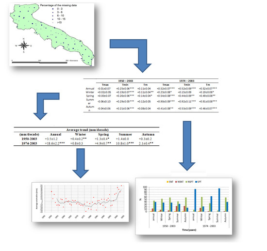
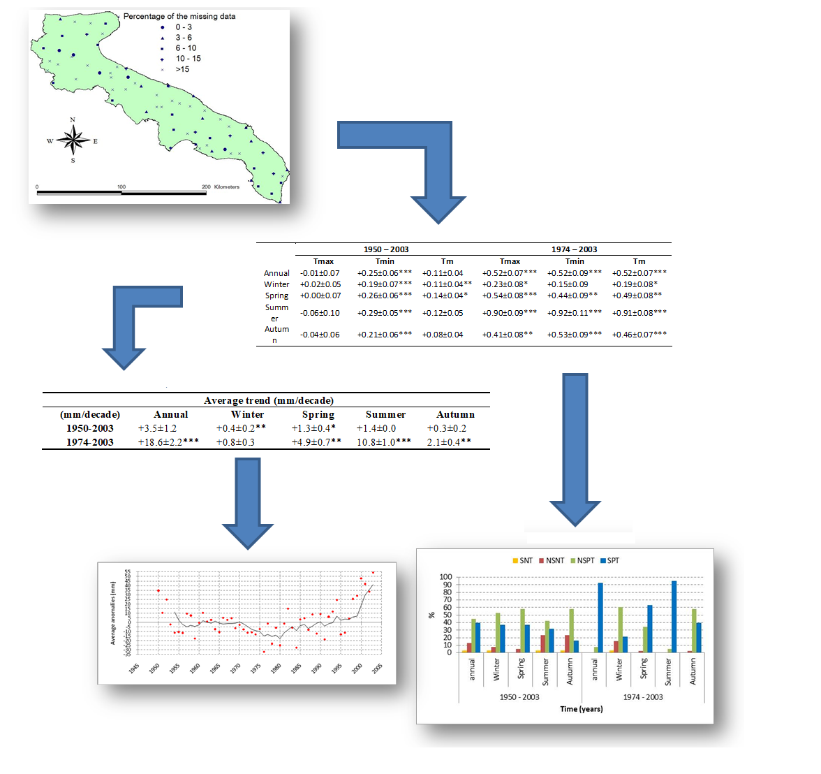
Figure 1. Distribution of the monitoring stations over the Apulia Region.
Sustainability 09 02337 g001
Figure 2. Temperature trend significance at 95% confidence level. Legend: SNT: Significant Negative Trend, NSNT: Non-Significant Negative Trend, NSPT: Non-Significant Positive Trend, SPT: Significant Positive Trend.
Sustainability 09 02337 g002
Figure 3. Spatial interpolation of the trend in °C/decade on a seasonal scale: the mean temperature.
Sustainability 09 02337 g003
Figure 4. Progressive trend analysis of the average mean temperature.
Sustainability 09 02337 g004
Figure 5. Progressive trend analysis of the average maximum and minimum temperatures (Tmax; Tmin).
Sustainability 09 02337 g005
Figure 6. Trend significance at a 99% confidence level of the reference evapotranspiration.
Sustainability 09 02337 g006
Figure 7. Anomalies of ETref (red box) with respect to the 1961–1990 base period and 5 days moving average (black line).
Sustainability 09 02337 g007
Table 1. Average trends in the study area (°C/decade).
1950–20031974–2003
TmaxTminTmTmaxTminTm
Annual−0.01 ± 0.07+0.25 ± 0.06 ***+0.11 ± 0.04+0.52 ± 0.07 ***+0.52 ± 0.09 ***+0.52 ± 0.07 ***
Winter+0.02 ± 0.05+0.19 ± 0.07 ***+0.11 ± 0.04 **+0.23 ± 0.08 *+0.15 ± 0.09+0.19 ± 0.08 *
Spring+0.00 ± 0.07+0.26 ± 0.06 ***+0.14 ± 0.04 *+0.54 ± 0.08 ***+0.44 ± 0.09 **+0.49 ± 0.08 **
Summer−0.06 ± 0.10+0.29 ± 0.05 ***+0.12 ± 0.05+0.90 ± 0.09 ***+0.92 ± 0.11 ***+0.91 ± 0.08 ***
Autumn−0.04 ± 0.06+0.21 ± 0.06 ***+0.08 ± 0.04+0.41 ± 0.08 **+0.53 ± 0.09 ***+0.46 ± 0.07 ***
Significance levels: *** <1%; ** 1–5%; * 5–10%.
Table 2. Temperatures average determination coefficient.
1950–20031974–2003
TmaxTminTmTmaxTminTm
Annual+0.10 ± 0.03+0.23 ± 0.06+0.10 ± 0.03+0.29 ± 0.05+0.37 ± 0.07+0.34 ± 0.06
Winter+0.05 ± 0.02+0.13 ± 0.04+0.06 ± 0.02+0.11 ± 0.03+0.09 ± 0.03+0.09 ± 0.03
Spring+0.06 ± 0.02+0.18 ± 0.05+0.07 ± 0.02+0.14 ± 0.03+0.16 ± 0.04+0.16 ± 0.03
Summer+0.09 ± 0.03+0.17 ± 0.04+0.07 ± 0.02+0.34 ± 0.04+0.45 ± 0.05+0.41 ± 0.04
Autumn+0.06 ± 0.02+0.11 ± 0.04+0.04 ± 0.01+0.13 ± 0.03+0.19 ± 0.04+0.15 ± 0.03
Table 3. Trend magnitude and significance of reference evapotranspiration.
Average Trend
(mm/Decade)AnnualWinterSpringSummerAutumn
1950–2003+3.5 ± 1.2+0.4 ± 0.2 **+1.3 ± 0.4 *+1.4 ± 0.0+0.3 ± 0.2
1974–2003+18.6 ± 2.2 ***+0.8 ± 0.3+4.9 ± 0.7 **10.8 ± 1.0 ***2.1 ± 0.4 **
Significance levels: *** <1%; ** 1–5%; * 5–10%.

