Optimal Reliable Point-in-Polygon Test and Differential Coding Boolean Operations on Polygons

Abstract

This paper provides a full theoretical and experimental analysis of a serial algorithm for the point-in-polygon test, which requires less running time than previous algorithms and can handle all degenerate cases. The serial algorithm can quickly determine whether a point is inside or outside a polygon and accurately determine the contours of input polygon. It describes all degenerate cases and simultaneously provides a corresponding solution to each degenerate case to ensure the stability and reliability. This also creates the prerequisites and basis for our novel boolean operations algorithm that inherits all the benefits of the serial algorithm. Using geometric probability and straight-line equation $F\left(P\right)=(y_i-y_{i+1})(x_p-x_i)-(y_i-y_p)(x_{i+1}-x_i)$, it optimizes our two algorithms that avoid the division operation and do not need to compute any intersection points. Our algorithms are applicable to any polygon that may be self-intersecting or with holes nested to any level of depth. They do not have to sort the vertices clockwise or counterclockwise beforehand. Consequently, they process all edges one by one in any order for input polygons. This allows a parallel implementation of each algorithm to be made very easily. We also prove several theorems guaranteeing the correctness of algorithms. To speed up the operations, we assign each vector a number code and derive two iterative formulas using differential calculus. However, the experimental results as well as the theoretical proof show that our serial algorithm for the point-in-polygon test is optimal and the time complexities of all algorithms are linear. Our methods can be extended to three-dimensional space, in particular, they can be applied to 3D printing to improve its performance.

1. Introduction

1.1. The Point-in-Polygon Test

Let P be a point and S a polygon on a plane. In computer graphics, finding whether P is inside, outside, or on the boundary of S is a fundamental problem, which is called the point-in-polygon test [1], point in polygon test [2], or inside-outside test [3] in different studies. In this paper, we call it the point-in-polygon test. Throughout this paper, let S denote a complex polygon that may be self-intersecting, concave, or have holes nested to any level of depth.

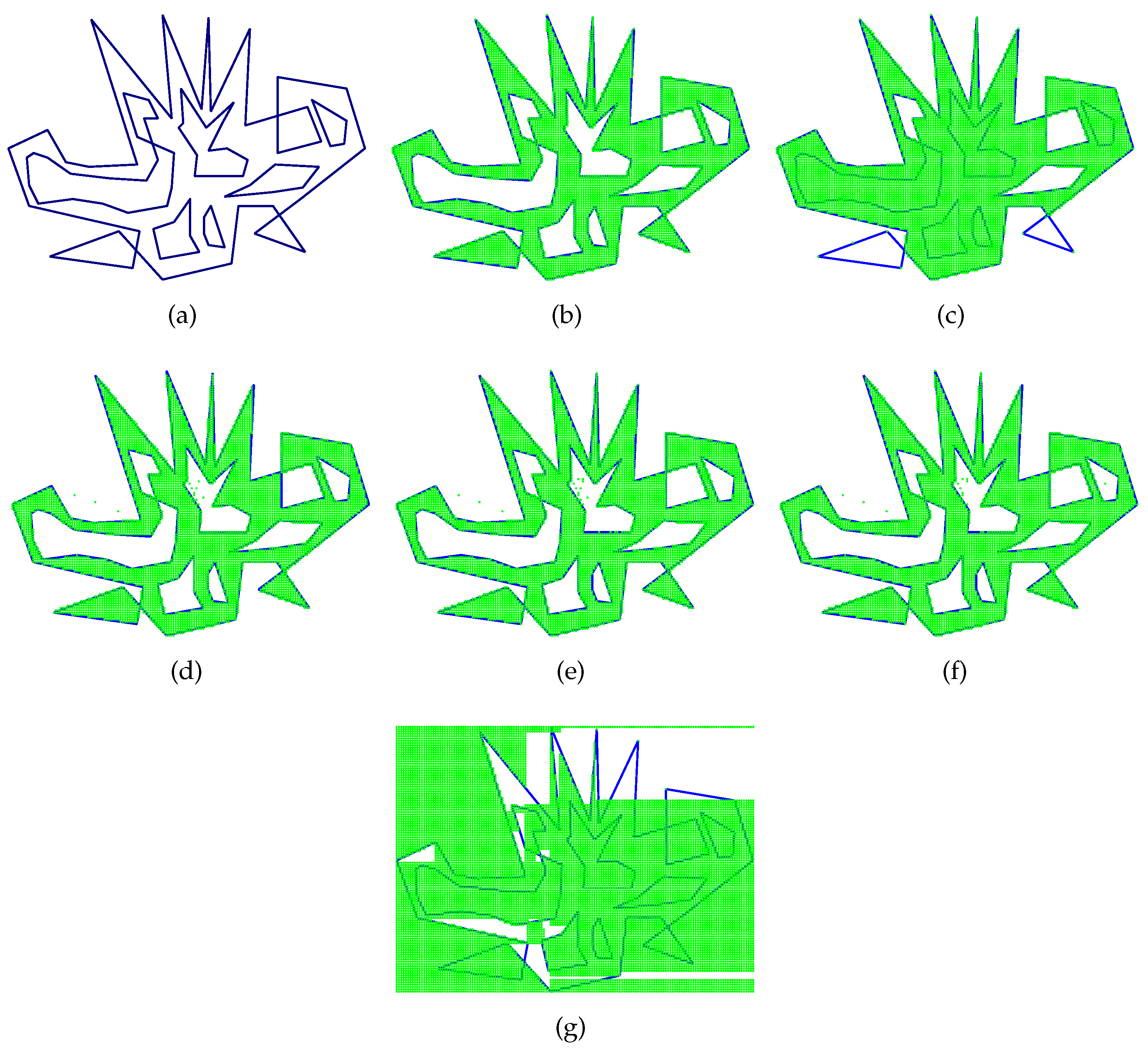
Currently, many algorithms are available for the point-in-polygon test. Jiménez et al. [1] improved the triangle-based algorithm and did not require any preprocessing, decomposition, or feature classification. However, they are sensitive to whether a polygon is clockwise or counterclockwise oriented and cannot be applied to a self-intersecting polygons or efficiently cope with degenerate cases (see Figure 1).

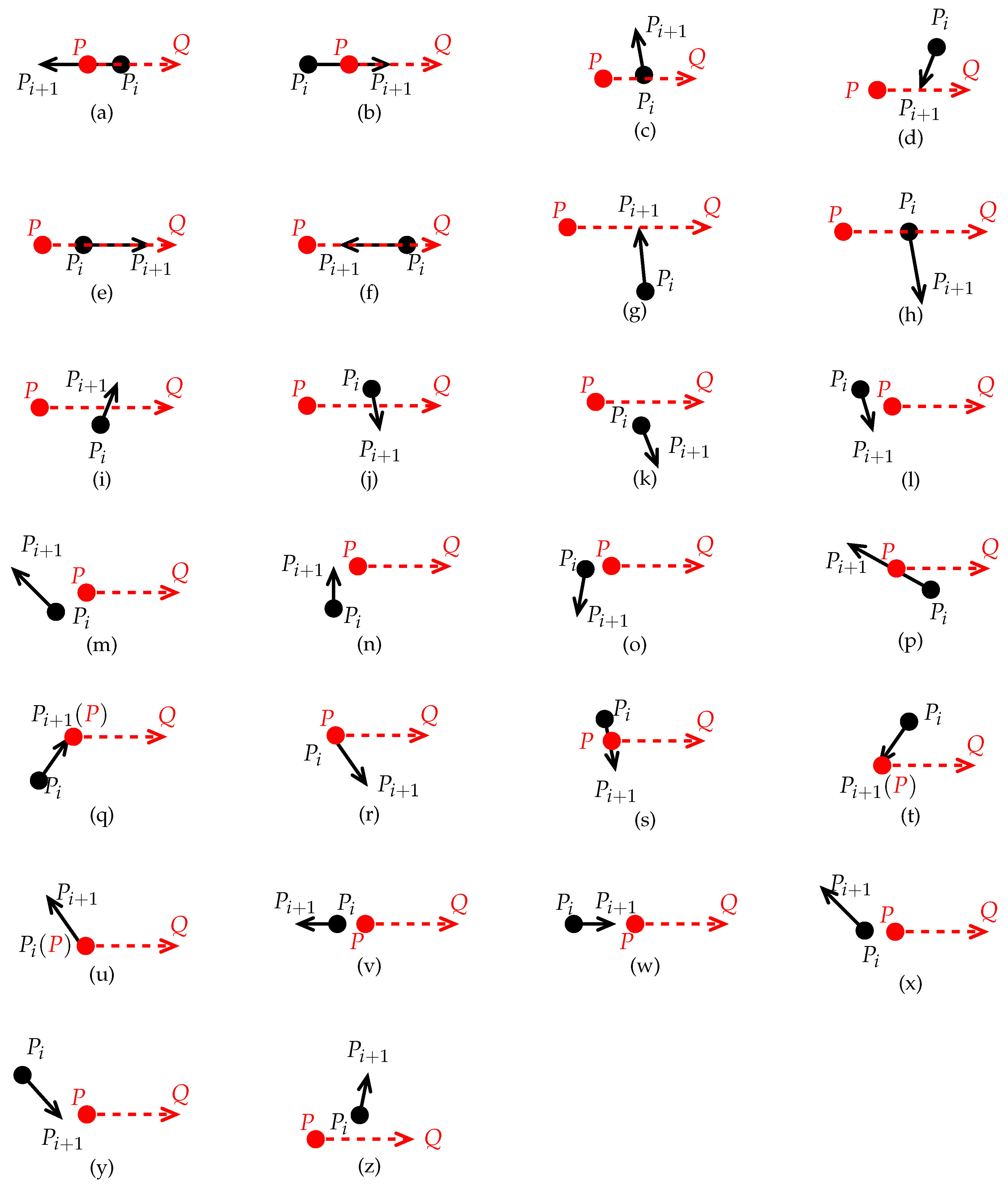
Presently, there is no ray-intersection algorithm that can handle all degenerate cases in which the tested point P is on $\partial S$ (the boundary of S). This includes the eight kinds of degenerate cases of the 26 kinds of positional relationships existing between $\overrightarrow{P_i{P}_{i+1}}$ and $\overrightarrow{PQ}$ , as shown in Figure 2a,b,p–u.

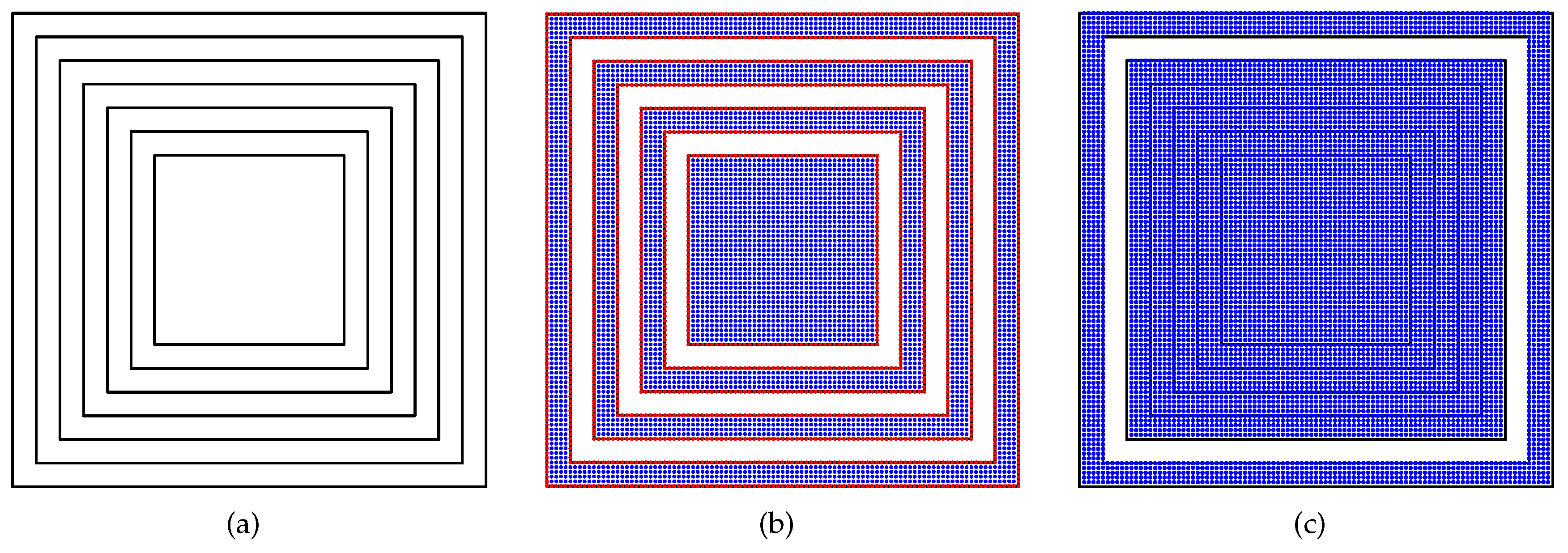
Despite many efforts [2,4], these approaches have the same problems as previous algorithms with degenerate cases (see Figure 1g). A detailed theoretical analysis and the proof of the correctness of the method for the point-in-polygon test are missing. In addition, apart from [4,5,6], few algorithms do not need to perform calculations for intersection points and costly division operations. However, these algorithms overlook some problems, such as how to identify a point lying on $\partial S$ and apply the point-in-polygon test for a polygon containing nested holes, as shown in Figure 3a. No attempt to optimize the algorithms for computing speed has been done.

Based on current knowledge, Haines [4,5] achieved the best performance. This algorithm is based on the ray intersection algorithm. This paper examines each aspect of the problem, including the various advantages and disadvantages of the previous algorithms, and provides a complete theoretical and experimental analysis. Finally, it presents a new algorithm for the point-in-polygon test that can handle all degenerate cases.

1.2. Boolean Operations

In computer graphics, boolean operations [3] on general polygons occur frequently in applications. The aim of boolean operations on polygons is to extract all contours of the resultant polygons or obtain all inner regions enclosed by the resultant polygons. If the goal is the latter, after the algorithm has extracted all contours of the resultant polygons, it would need to perform additional processing steps, such as scan-conversion or area-filling.

A traditional algorithm should follow the five main steps below: computing, ordering, traversing, tracking intersection points, and establishing contours. When degenerate cases occur, Weiler [7] would require special steps to be taken to deal with them. A more detailed discussion about the issue is beyond the scope of this article. The main problem encountered by boolean operation algorithms is that, because any two edges from different input polygons may overlap each other, the calculation of intersection points becomes more complicated and may cause program instability.

This paper considers the point-in-polygon test and the rasterization algorithm, and presents a novel method that can simultaneously perform both tasks, extracting the polygon boundaries and obtaining the interior regions. Our method can be applied to 3D printing [8] to improve its performance. We compare this method with that in [9], and find that there are some commonalities, but they are actually considerably different.

1.3. The Major Contributors of This Paper

The major contributions of this paper are as follows.

• For the point-in-polygon test, it provides a full theoretical and experimental analysis and presents the serial Algorithm 1, which requires less running time than previous algorithms, can handle all degenerate cases, and can both quickly determine whether a point is inside or outside a polygon and accurately determine the contours of input polygon (see the example in Figure 3b).
• It describes all degenerate cases and provides corresponding solutions to ensure the stability and reliability (see Figure 2). This also creates the prerequisites and basis for our boolean operations algorithm.
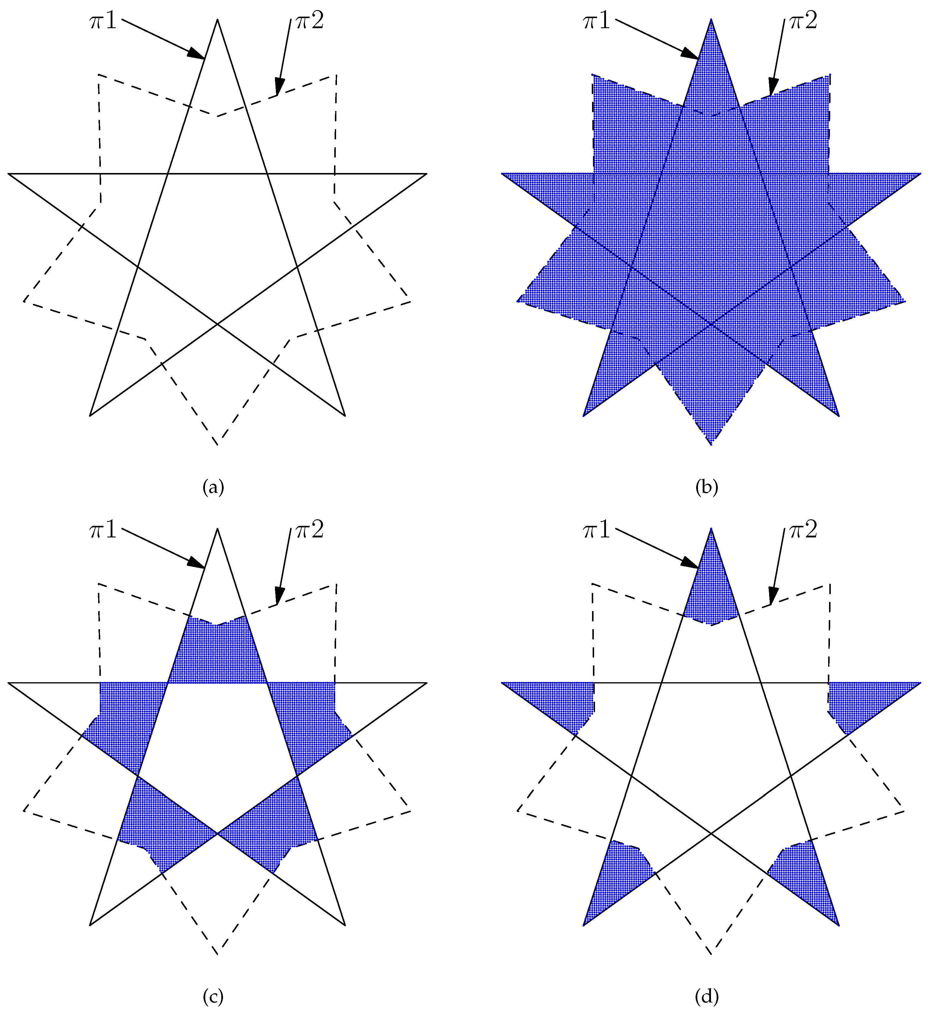
• It also presents a novel Algorithm 2 for boolean operations, as shown in Figure 4.
• Our algorithms avoid the division operation and expensive intersection calculations, do not have to sort the vertices clockwise or counterclockwise beforehand, process all edges one by one in any order for an input polygon, are parallelizable because their many operations can be done in parallel, and are applicable to any polygons, including self-intersecting polygons or those with holes nested to any level of depth (see Figure 3).
• To speed up boolean operations, it provides each vector a number code (see Figure 2) and derives two iterative formulas (Equations (4) and (5)) using differential calculus.
• A detailed theoretical and experimental analysis of Algorithms 1 and 2, including the proofs of their correctness (see Theorems 1–4), are shown.
• Using geometric probability and Equation (3), it optimizes all algorithms.

2. Related Work

2.1. The Point-in-Polygon Test

By examining theoretical principles and technical features, we can classify the existing algorithms into the following five categories:

• Ray-intersection algorithm

In many studies, this type of algorithm is called the ray–crossing [2], crossings–count [4], odd–even [3], odd parity [3], or even–odd [2,10] algorithm because the structures and principles of the different algorithms are all slightly different. However, virtually all of these algorithms evolved from the ray-intersection algorithm, which works by shooting a ray $\overrightarrow{PQ}$ in any direction (see Figure 5; in general, this is done parallel to the x-axis) from the test point P to infinity and counts the number of intersections between the ray $\overrightarrow{PQ}$ and all edges of input polygon. Wang et al. [11] classified edges into layers and calculated the number of intersections, but did not apply to self-intersecting polygons. Moreover, the time complexities of the preprocessing steps ranges from $O\left(n\right)$ to $O\left(n^2\right)$, depending on the polygon shape and the test direction.

If the boundary curve is represented as a spline curve, then the ray-intersection algorithm can be easily modified as one only needs to compute the intersection points with a spline curve and that can be easily achieved by efficient root-finding algorithms [12,13,14,15].

The paper considers the multiplicity of the ray-vs.-edge intersection as shown in Figure 2c–z, in particular in Figure 2c–j. Further, the proof of Lemma 1 also provides relevant evidence and reasons in detail.

• Sum of angles algorithm

The sum of angles algorithm [1] is equivalent to the angle summation algorithm [2], which needs to calculate the angle sum of a polygon. Thus, the algorithms carry out trigonometric operations that lead to floating-point operations and have substantial time and space costs.

• Winding number algorithms

The winding number algorithm [2], also called the nonzero winding number algorithm [3], includes two approaches: the first is an improved algorithm from the sum of angles that introduces the cross and dot product operations of two vectors and thereby avoids angle calculations [3]. However, if the two vectors are parallel or vertical, the calculations would fail. In addition, if the input polygon is self-intersecting or has holes, the results would be incorrect. By improving the even-odd algorithm step by step, the second approach shows the even-odd and the nonzero winding number algorithms are identical except in their interpretation of the intersection count [2].

• Grid algorithm

Gombos˘i and Žalik [16] considered a polygon as a group of grid cells and used $O\left(n\sqrt{n}\right)$ time to first preprocess a given polygon. Following the rule in [16], the quasi-closest point algorithm must also be preprocessed to subdivide the bounding rectangle of a polygon into uniform-sized cells [17]. However, this method can only be used on raster-based problems and cannot be used on self-intersecting polygons.

• Decomposition algorithm

The decomposition algorithms with $O(nlogn)$ time complexity must perform preprocessing to partition an input polygon into a series of simpler components, including trapezoids (swaths) [18], convex sub-polygons, quad meshes, or triangles (tri-cones) [1]. The multi-$L-REP$ [19] and the $EL-REP$ [20] algorithms extended the $L-REP$ decomposition algorithm. At worst, the latter has time complexity $O\left({log}^{2}n\right)$.

2.2. Boolean Operations

Many available algorithms exist for boolean operations, but some of them have limitations on the shape of input polygons. For example, Andreev [21] required a rectangular clip polygon, while Rappoport [22] required a convex clip polygon. Greiner and Hormann [23] handled degenerate cases by perturbing the position of the vertex, but, by doing so, it required some additional computational overhead, which makes its running time undeterminable. Weiler [7], Weiler and Atherton [24], and Andreev [21] permitted any clip or subject polygons to be concave or with holes, but could not handle self-intersecting polygons. Vatti [25] and Greiner and Hormann [23] could perform boolean operations for any clip and subject polygons including those that are self-intersecting, concave, or with holes.

Vatti [25] used the plane sweep technique [9]. Martínez et al. [26] subdivided the edges of polygons at the points of intersection. Therefore, the algorithm must be modified when it encounters self-intersecting or unexpected input polygons, such as two edges overlapping.

Based on simple chains [27], Rivero and Feito [28] could avoid the treatment of degenerate cases. However, the approach is invalid for self-intersecting polygons. The execution time of [29] is less than one-third of that of [28]. Weiler [7] provided an improvement over [24]. However, Weiler [7] could not handle self-intersecting polygons.

Graysmith and Shaw [30] performed boolean operations by dividing the geometric shape into a set of meshes. Although the plane sweep algorithm [9] attempts to do this, it does not satisfy the necessary conditions.

3. The Point-in-Polygon Test Principle

Definition 1.

A polygon S is composed of rings. A $ring$ is a sequence of edges, which link together and form a closed circuit. A ring containing all other rings is the $outer$ $ring$ of S, while each of the remaining rings is the $inner$ $ring$ of S, also known as $inner$ $hole$ of S, and referred to as $hole$ of S.

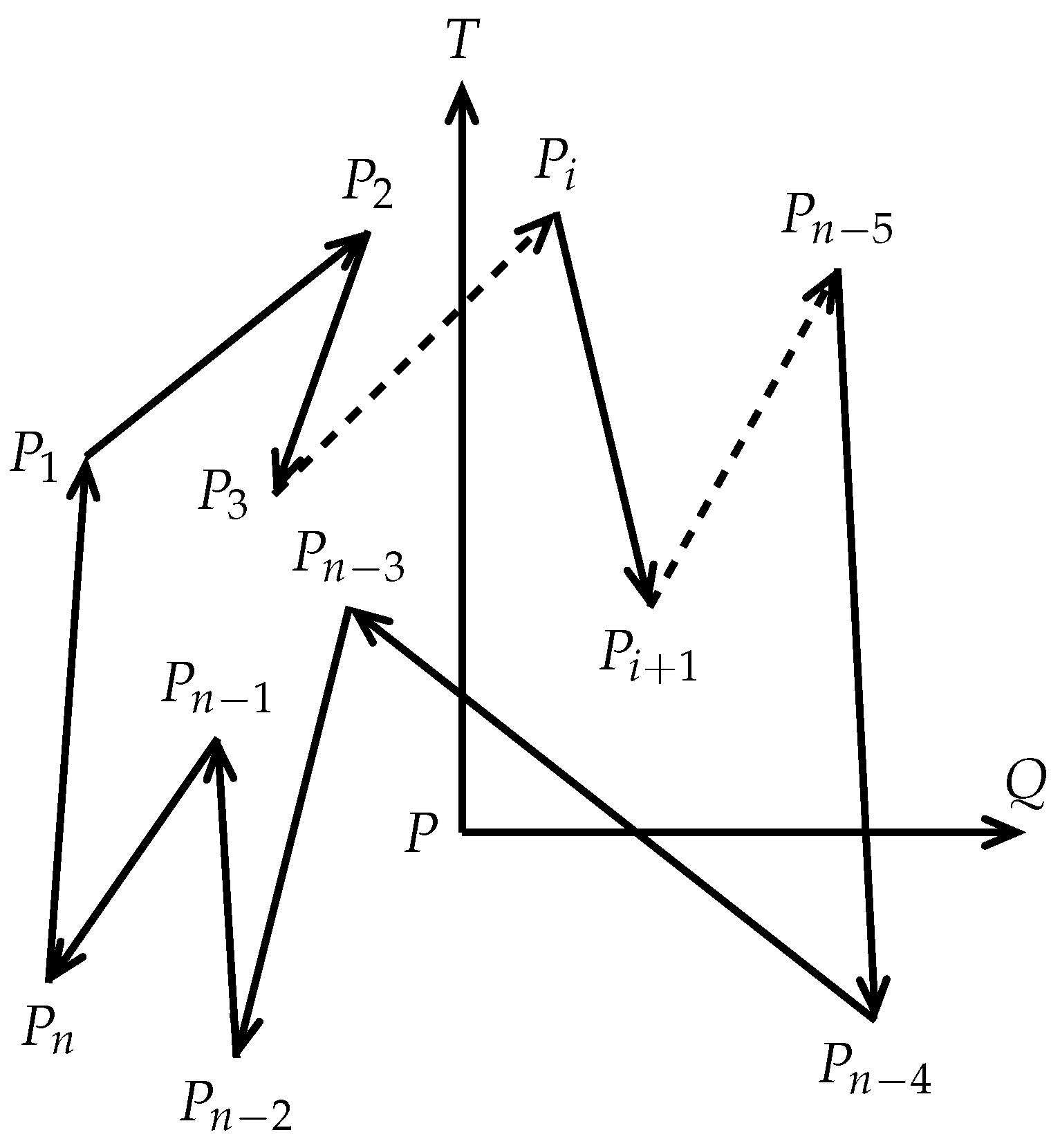
Let S be a closed polygon on a plane with n vertices $P_1(x_1,y_1)$, $P_2(x_2,y_2),$ $\cdots ,P_i(x_i,y_i)$, $\cdots ,P_n(x_n,y_n)$ such that there exists an edge between $P_i$ and $P_{i+1}$ for all $i\in \{1,2,\cdots ,n-1\}$ and between $P_n$ and $P_1$ (see Figure 5). Let $\overrightarrow{P_i{P}_{i+1}}$ be an edge vector of S. Let $P(x,y)$ be a point on the plane. We define a function $F(x,y)$ as follows:

$$\begin{array}{cc}\hfill F(x,y)& =(x_{i+1}-x_i)y-(y_{i+1}-y_i)x+x_i{y}_{i+1}-x_{i+1}{y}_i\hfill \end{array}$$

(1)

$$\begin{array}{c}=(y_i-y_{i+1})(x-x_i)-(y_i-y)(x_{i+1}-x_i).\hfill \end{array}$$

(2)

Equation (1) requires one addition, four subtractions, four multiplications, and a total of nine operations while Equation (2) requires only five subtractions, two multiplications, and a total of seven operations. In addition, we know that multiplication takes more time than addition or subtraction. Therefore, to reduce the running times of our algorithms below, we always use Equation (2).

Definition 2.

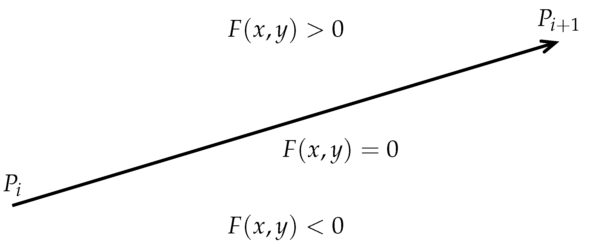
Given an edge vector $\overrightarrow{P_i{P}_{i+1}}$ whose function $F(x,y)=(y_i-y_{i+1})(x-x_i)-(y_i-y)(x_{i+1}-x_i)$ with $P_i=(x_i,y_i)$ and $P_{i+1}=(x_{i+1},y_{i+1})$.

$F(x,y)$ satisfying the Jordan property means that the edge vector $\overrightarrow{P_i{P}_{i+1}}$ divides the plane into two half plane that are disconnected from each other (see Figure 6). Therefore, $F(x,y)$ satisfying the Jordan property can also be called the vector $\overrightarrow{P_i{P}_{i+1}}$ satisfies Jordan property.

Assume that $\overrightarrow{PQ}$ is a horizontal ray that starts at $P(x_p,y_p)$, passes through $Q(x_q,y_q)$, and extends infinitely in the $+x$ direction (see Figure 5). We define a variable $k=0$ to accumulate the total number of intersections made by $\overrightarrow{PQ}$ and all edges of S. By (2) for $\overrightarrow{PQ}$ , it follows that

$$\begin{array}{ccc}\hfill F(x,y)& =& (y_p-y_p)(x-x_p)-(y_p-y)(x_q-x_p)\hfill \\ & =& (x_q-x_p)(y-y_p).\hfill \end{array}$$

because $(x_q-x_p)>0$, $F(x,y)$ and $(y-y_p)$ are either all positive or all negative. For $P_i(x_i,y_i)$ with $i\in \{1,2,\cdots ,n\}$, if $y_i>y_p$, then $P_i$ is on the left side of $\overrightarrow{PQ}$ (above). Otherwise, if $y_i<y_p$, then $P_i$ is on the right side of $\overrightarrow{PQ}$ (below). If neither is true, then $P_i$ is on the ray $\overrightarrow{PQ}$. By substituting $P(x_p,y_p)$ into Equation (2), we establish the following equation.

$$F\left(P\right)=(y_i-y_{i+1})(x_p-x_i)-(y_i-y_p)(x_{i+1}-x_i).$$

(3)

Starting from the point $P_1$, we traverse each edge vector $\overrightarrow{P_i{P}_{i+1}}$ of S exactly once and manage to determine the positional relationship between $\overrightarrow{P_i{P}_{i+1}}$ and $\overrightarrow{PQ}$ . Thus, without calculating the intersection point, one can accurately determine whether $\overrightarrow{P_i{P}_{i+1}}$ and $\overrightarrow{PQ}$ intersect each other. Furthermore, if $\overrightarrow{P_i{P}_{i+1}}$ and $\overrightarrow{PQ}$ intersect each other, we set $k=k+1$. By carefully analyzing whether $\overrightarrow{PQ}$ and $\overrightarrow{P_i{P}_{i+1}}$ intersect each other, and whether the point P is on $\overrightarrow{P_i{P}_{i+1}}$ , it can be seen that $\overrightarrow{PQ}$ with $\overrightarrow{P_i{P}_{i+1}}$ can have the following 26 different positional relationships (see Figure 2).

• $x_{i+1}\le x_p\le x_i\wedge y_{i+1}=y_p=y_i$, P is on $\overrightarrow{P_i{P}_{i+1}}$ (see Figure 2a). Thus, P is on $\partial S$.
• $x_i\le x_p\le x_{i+1}\wedge y_i=y_p=y_{i+1}$, P is on $\overrightarrow{P_i{P}_{i+1}}$ (see Figure 2b. Thus, P is on $\partial S$.
• $F\left(P\right)>0\wedge y_i=y_p\wedge y_p<y_{i+1}$, P is on the back-left side of $\overrightarrow{P_i{P}_{i+1}}$ ( the viewing direction is along the direction of $\overrightarrow{P_i{P}_{i+1}}$ , which is maintained below. see Figure 2c). Thus, $\overrightarrow{P_i{P}_{i+1}}$ intersects $\overrightarrow{PQ}$ and we set $k=k+1$.
• $F\left(P\right)<0\wedge y_i>y_p\wedge y_p=y_{i+1}$, P is on the front-right side of $\overrightarrow{P_i{P}_{i+1}}$ (see Figure 2d). Thus, $\overrightarrow{P_i{P}_{i+1}}$ intersects $\overrightarrow{PQ}$ and we set $k=k+1$.
• $y_p=y_i=y_{i+1}\wedge x_{i+1}>x_i>x_p$, $\overrightarrow{P_i{P}_{i+1}}$ and $\overrightarrow{PQ}$ have the same direction, and the edge $\overline{P_i{P}_{i+1}}$ is shorter than the edge $\overline{PQ}$ (see Figure 2e). Although both overlap each other on $\overline{P_i{P}_{i+1}}$, we regard them as having no intersection, and k remains unchanged.
• $y_p=y_i=y_{i+1}\wedge x_i>x_{i+1}>x_p$, $\overrightarrow{P_i{P}_{i+1}}$ overlaps $\overrightarrow{PQ}$ , and both have opposite directions (see Figure 2f). Although both overlap on $\overrightarrow{P_i{P}_{i+1}}$ , we regard them as having no intersection, and remain k unchanged.
• $F\left(P\right)>0\wedge y_p=y_{i+1}\wedge y_{i+1}>y_i$, P is on the front-left side of $\overrightarrow{P_i{P}_{i+1}}$ (see Figure 2g). Although $\overrightarrow{P_i{P}_{i+1}}$ intersects $\overrightarrow{PQ}$ at $P_{i+1}$, we regard them as having no intersection, and k remains unchanged.
• $F\left(P\right)<0\wedge y_p=y_i\wedge y_i>y_{i+1}$, P is on the back-right side of $\overrightarrow{P_i{P}_{i+1}}$ (see Figure 2h). Although $\overrightarrow{P_i{P}_{i+1}}$ intersects $\overrightarrow{PQ}$ at $P_i$, we regard them as having no intersection, and k remains unchanged (similar to Case 7).
• $F\left(P\right)>0\wedge y_{i+1}>y_p>y_i$, P is on the left-middle side of $\overrightarrow{P_i{P}_{i+1}}$ (see Figure 2i). Thus, $\overrightarrow{P_i{P}_{i+1}}$ intersects $\overrightarrow{PQ}$ , and we set $k=k+1$.
• $F\left(P\right)<0\wedge y_i>y_p>y_{i+1}$, P is on the right-middle side of $\overrightarrow{P_i{P}_{i+1}}$ (see Figure 2j). Thus, $\overrightarrow{P_i{P}_{i+1}}$ intersects $\overrightarrow{PQ}$ , and we set $k=k+1$.
• $y_p>y_i\wedge y_p>y_{i+1}$, $\overrightarrow{P_i{P}_{i+1}}$ is on the right side of $\overrightarrow{PQ}$ (below) (see Figure 2k). Thus, both are disjoint, and k remains unchanged.
• $F\left(P\right)>0\wedge y_p<y_i\wedge y_{i+1}<y_p$, $\overrightarrow{PQ}$ is also on the left side of $\overrightarrow{P_i{P}_{i+1}}$ (see Figure 2l). Thus, both are disjoint, and k remains unchanged.
• $F\left(P\right)<0\wedge y_p<y_{i+1}\wedge y_p>y_i$, $\overrightarrow{PQ}$ is on the right side of $\overrightarrow{P_i{P}_{i+1}}$ (see Figure 2m). Thus, both are disjoint, and k remains unchanged.
• $F\left(P\right)<0\wedge y_p=y_{i+1}\wedge y_p>y_i$, $\overrightarrow{PQ}$ is on the right side of $\overrightarrow{P_i{P}_{i+1}}$ (see Figure 2n). Thus, both are disjoint, and k remains unchanged.
• $F\left(P\right)>0\wedge y_p=y_i\wedge y_p>y_{i+1}$, $\overrightarrow{PQ}$ is on the left side of $\overrightarrow{P_i{P}_{i+1}}$ (see Figure 2o). Thus, both are disjoint, and k remains unchanged.
• $F\left(P\right)=0\wedge y_i<y_p\wedge y_p<y_{i+1}$, P is on $\partial S$ $\overrightarrow{P_i{P}_{i+1}}$ (see Figure 2p).
• $P=P_{i+1}\wedge y_p>y_i$, P is on $\partial S$ $\overrightarrow{P_i{P}_{i+1}}$ (see Figure 2q).
• $P=P_i\wedge y_p>y_{i+1}$, P is on $\partial S$ $\overrightarrow{P_i{P}_{i+1}}$ (see Figure 2r).
• $F\left(P\right)=0\wedge y_i>y_p\wedge y_p>y_{i+1}$, P is on $\partial S$ $\overrightarrow{P_i{P}_{i+1}}$ (see Figure 2s).
• $P=P_{i+1}\wedge y_p<y_i$, P is on $\partial S$ $\overrightarrow{P_i{P}_{i+1}}$ (see Figure 2t).
• $P=P_i\wedge y_p<y_{i+1}$, P is on $\partial S$ $\overrightarrow{P_i{P}_{i+1}}$ (see Figure 2u).
• $y_p=y_i=y_{i+1}\wedge x_{i+1}<x_i<x_p$, $\overrightarrow{P_i{P}_{i+1}}$ and $\overrightarrow{PQ}$ are mutually separate, and both have opposite directions $\overrightarrow{P_i{P}_{i+1}}$ (see Figure 2v). Thus, they are disjoint, and k remains unchanged.
• $y_p=y_i=y_{i+1}\wedge x_p>x_{i+1}>x_i$, $\overrightarrow{P_i{P}_{i+1}}$ and $\overrightarrow{PQ}$ are disjoint $\overrightarrow{P_i{P}_{i+1}}$ (see Figure 2w), and k remains unchanged.
• $F\left(P\right)<0\wedge y_i=y_p\wedge y_p<y_{i+1}$, P is on the back-right side of $\overrightarrow{P_i{P}_{i+1}}$ , and $\overrightarrow{P_i{P}_{i+1}}$ and $\overrightarrow{PQ}$ are disjoint $\overrightarrow{P_i{P}_{i+1}}$ (see Figure 2x). Thus, k remains unchanged.
• $F\left(P\right)>0\wedge y_{i+1}=y_p\wedge y_p<y_i$, P is on the front-left side of $\overrightarrow{P_i{P}_{i+1}}$ , and $\overrightarrow{P_i{P}_{i+1}}$ and $\overrightarrow{PQ}$ are disjoint $\overrightarrow{P_i{P}_{i+1}}$ (see Figure 2y). Thus, k remains unchanged.
• $y_p<y_i\wedge y_p<y_{i+1}$, $\overrightarrow{P_i{P}_{i+1}}$ is on the left side of $\overrightarrow{PQ}$ (above), and $\overrightarrow{P_i{P}_{i+1}}$ and $\overrightarrow{PQ}$ are disjoint $\overrightarrow{P_i{P}_{i+1}}$ (see Figure 2z). Thus, k remains unchanged.

Further, we can classify and simplify the 26 positional relationships into three classes:

• Class 1 includes Cases 3, 4, 9, and 10, for each of which $\overrightarrow{P_i{P}_{i+1}}$ intersects $\overrightarrow{PQ}$ . Therefore, we set $k=k+1$.
• Class 2 includes Cases 1, 2, and 16–21, for each of which P is on $\partial S$.
• Class 3 includes the remaining cases, for each of which $\overrightarrow{P_i{P}_{i+1}}$ and $\overrightarrow{PQ}$ are disjoint. Therefore, k remains unchanged.

To facilitate the analysis and processing of the problem, we give each vector involved in these operations a number code of 1–26 such that each vector $\overrightarrow{P_i{P}_{i+1}}$ in Figure 2a–z has a number code of 1–26, which is one-to-one correspondence with Cases 1–26.

Definition 3.

Let S consist of a set of closed polygons. The minimum bounding box of S, denoted by $MBB$, is the smallest box that encloses the entire S and is axis-aligned rather than oriented-aligned.

For the point-in-polygon test and boolean operations, our methodology can be divided into two steps. The first step performs preprocessing to determine whether a point lies inside or outside the minimum bounding box $MBB$ of input polygons. If the point lies within the $MBB$, we then perform the second step to determine whether the point is inside or outside the polygon.

Occasionally, a user may need to handle polygons with small sizes. Clearly, the occurrence probability of input polygons with limited sizes, involved in operations, is low. For example, let us consider the possibility of occurrence that the input polygon has vertices (0,0), (1,1), (1,$1-t$) with small t. It is true that this probability is tiny. Furthermore, it follows that the probability of a point lying on the boundary of a polygon is approximately zero, since the actual width the edge of a polygon in use is not 0.

To optimize our algorithms, we can let the program automatically calculates the probabilities of a point lying within and outside a polygon. If the probability of the point lying within the polygon is greater than the probability of the point lying outside the polygon when the minimum bounding box $MBB$ has been calculated, we let the program first decide whether the point is within the polygon, and then decide whether the point is outside the polygon. Conversely, if the probability of the point lying outside the polygon is greater than the probability of the point lying within the polygon, we let the program first decide whether the point is outside the polygon, and then decide whether the point is within the polygon. Since the probability of the point lying on the boundary of the polygon is approximately zero, we let the program at last decide whether the point is on the polygon. In this paper, we assume that the probability of a point lying within a polygon is greater than the probability of the point lying outside the polygon.

Definition 4.

Let S be a closed polygon and P a point on the plane. If P is on an edge of S, then we set $k=-1$. Otherwise, we set k equal to the number of intersections made by the ray $\overrightarrow{PQ}$ and all edges of S. We define the variable k as the point P is odd-even number around S, referred to as the point P is odd-even number, denoted by $S\left(P\right)$.

In addition, when P is inside the $outer$ $ring$ of S (see Definition 1), if the k is even, then we call P outside S. On the contrary, if the k is odd, then we call P inside S.

Lemma 1.

Let S be a closed polygon and P a point on the plane. By Definition 1, assume that Γ is a ring of S, which intersects with $\overrightarrow{PQ}$ . Assume that $U_1,U_2,\cdots ,U_t$ are all intersections produced by $\overrightarrow{PQ}$ and all edges of Γ with $t\ne 0$. Then, the P is outside Γ if and only if the t is an even.

Proof. 

By the conditions of Lemma 1, we have that $U_1(x_1,y_1),U_2(x_2,y_2),\cdots ,U_t(x_t,y_t)$ are the intersections produced by $\overrightarrow{PQ}$ and all edges of $\Gamma$. In Figure 2a–z, it can be observed that $\overrightarrow{PQ}$ and just the $\overrightarrow{P_i{P}_{i+1}}$ in Figure 2c,d,i or Figure 2j can have intersections.

Let us first prove the necessity. Suppose the P is outside S.

At first, we let $U=U_1$ and $k=1$. For the intersections U, our proof is divided into the following two main steps.

• If the intersection of $\overrightarrow{PQ}$ and the $\overrightarrow{P_i{P}_{i+1}}$ (denoted by $I_9{J}_{10}$) in Figure 2i or Figure 2j is U, then $I_9{J}_{10}$ crosses $\overrightarrow{PQ}$ from one side to another. Since $I_9{J}_{10}$ belongs to the closed $\Gamma$, there must be another edge $\overrightarrow{P_i{P}_{i+1}}$ in Figure 2c,d,i, or Figure 2j that also intersects with $\overrightarrow{PQ}$ at another different intersection (denoted by $V_1$). Let us assume that $V_1=U_2$. Therefore, $k=k+1=2$.
• Otherwise, if the intersection of $\overrightarrow{PQ}$ and the $\overrightarrow{P_i{P}_{i+1}}$ (denoted by $C_3{D}_4$) in Figure 2c or Figure 2d is U, then the other side connecting to U(denoted by $U38$) can only be the $\overrightarrow{P_i{P}_{i+1}}$ in Figure 2c–g, or Figure 2h.
  Besides, our proof for Lemma 1 is divided into the following three main sub-steps.

  (a)

  If $U38$ is the $\overrightarrow{P_i{P}_{i+1}}$ (denoted by $C_3^1{D}_4^1$) in Figure 2c or Figure 2d, then $\overrightarrow{PQ}$ and $C_3^1{D}_4^1$ must produce a new intersection (denoted by $V_2$), which is equal to U and let us assume that $V_2=U_2$. $U_2$ increases the number of intersections of $\Gamma$ and $\overrightarrow{PQ}$ by 1. Therefore, $k=k+1=2$.

  (b)

  Otherwise, if $U38$ is the $\overrightarrow{P_i{P}_{i+1}}$ (denoted by $E_5{F}_6$) in Figure 2e or Figure 2f, then $E_5{F}_6$ belongs to the closed $\Gamma$ of S. Then, next, the other side connecting to $E_5{F}_6$ (denoted by $U{38}^1$) can only be the $\overrightarrow{P_i{P}_{i+1}}$ in Figure 2c–g, or Figure 2h.

  • If $U{38}^1$ is the $\overrightarrow{P_i{P}_{i+1}}$ (denoted by $C_3^2{D}_4^2$) in Figure 2c or Figure 2d, then $\overrightarrow{PQ}$ and $C_3^2{D}_4^2$ must produce a new intersection, which is different from U (denoted by $V_3$). Let us assume that $V_3=U_2$. Therefore, $k=k+1=2$.
  • Otherwise, if $U{38}^1$ is the $\overrightarrow{P_i{P}_{i+1}}$ (denoted by $E_3^1{F}_4^1$) in Figure 2e or Figure 2f, the procedure returns to Step 2b above. Since the number of edges of $\Gamma$ is limited, this iteration will end after finite number of steps.
  • Otherwise, if $U{38}^1$ is the $\overrightarrow{P_i{P}_{i+1}}$ (denoted by $G_7{H}_8$) in Figure 2g or Figure 2h, then the path $C_3{D}_4\to E_5{F}_6\to G_7{H}_8$ crosses $\overrightarrow{PQ}$ from one side to another. Since $G_7{H}_8$ belongs to the closed $\Gamma$ of, there must be another edge $\overrightarrow{P_i{P}_{i+1}}$ in Figure 2c,d,i, or Figure 2j that also intersects with $\overrightarrow{PQ}$ at another different intersection (denoted by $V_4$). Let us assume that $V_4=U_2$. Therefore, $k=k+1=2$.

  (c)

  Otherwise, if $U38$ is the $\overrightarrow{P_i{P}_{i+1}}$ (denoted by $G_7{H}_8$) in Figure 2g or Figure 2h, the path $C_3{D}_4\to G_7{H}_8$ crosses $\overrightarrow{PQ}$ from one side to another. Since $G_7{H}_8$ belongs to the closed $\Gamma$, there must be another edge $\overrightarrow{P_i{P}_{i+1}}$ in Figure 2c,d,i, or Figure 2j that also intersects with $\overrightarrow{PQ}$ at another different intersection (denoted by $V_5$). Let us assume that $V_5=U_2$. Therefore, $k=k+1=2$.

From the intersection sequence $U_1,U_2,\cdots ,U_t$, we remove $U_1$ and $U_2$, and let $U=U_3$ and k = k + 1. Then, we repeat the above Steps 1 and 2 until there is no intersection in the intersection sequence $U_1,U_2,\cdots ,U_t$. Finally, it can be seen that the conclusion of Lemma 1 holds.

Let us prove the sufficiency in Lemma 1. Suppose the t is even.

We use the induction for $m=t/2$.

If $m=1$, by Figure 2a–z, suppose the pair of intersections are $U_1$ and $U_2$. Further, let us assume that $U=U_1$, then $U_2$ must belong to an element of $S_1=\{V_1,V_2,V_3,V_4,V_5\}$ (see the proof of the necessity of Lemma 1). Regardless of which element $U_2$ belongs to $S_1$, eventually it can be seen that P is outside $\Gamma$. Therefore, it is established that P is outside $\Gamma$ for $m=1$.

Suppose that P is outside $\Gamma$ for $m=k$.

Let us prove that P is outside $\Gamma$ for $m=k+1$.

Suppose that there exists a point that is outside $\Gamma$ for $m=k$; it can be asserted that there is always a point $P_0(x_0,y_0)$ outside $\Gamma$ such that the number of pairs of intersection points of $\overrightarrow{P_{0}Q}$ and $\Gamma$ is k.

Assume that only the x coordinate of the two intersections $U_1(x_1,y_1)$ and $U_2(x_2,y_2)$ is less than the x coordinate of any other intersection, and $U_1(x_1,y_1)$ and $U_2(x_2,y_2)$ meet condition $x_1\le x_2$.

Further, let us assume that $U=U_1$, then $U_2$ must belong to an element of $S_1=\{V_1$, $V_2$, $V_3$, $V_4$, $V_5\}$ (see the proof of the necessity of Lemma 1). Regardless of which element $U_2$ belongs to $S_1$, on the ray $\overrightarrow{PQ}$ , there is only one pair of intersections $U_1(x_1,y_1)$ and $U_2(x_2,y_2)$ produced by $\overrightarrow{P{P}_0}$ and all edges of $\Gamma$. Therefore, it can be inferred that P is outside $\Gamma$.

Eventually, it can be seen that P is outside $\Gamma$ for $m=k+1$. Therefore, it is established that P is outside $\Gamma$ for $m=k+1$. □

Lemma 2.

Let S be a closed polygon and P a point on the plane. By Definition 1, assume that Γ is a ring of S, which intersects with $\overrightarrow{PQ}$ . Assume that $U_1,U_2,\cdots ,U_t$ are all intersections produced by $\overrightarrow{PQ}$ and all edges of Γ with $t\ne 0$. Then, P is inside Γ if and only if the t is an odd.

Proof. 

Let us first prove the necessity. Suppose the P is inside $\Gamma$. We now prove the necessity of Lemma 2 by contradiction. Assume by contradiction that the t is an even.

Then, by the sufficiency of Lemma 1, it follows that the P is outside $\Gamma$, leading to a contradiction with the constraint that the P is inside $\Gamma$. Therefore, the assumption that the t is an even does not hold. The necessity of Lemma 2 immediately follows.

Next, let us prove the sufficiency in Lemma 2. Suppose the t is an odd. We now prove the sufficiency of Lemma 2 by contradiction. Assume by contradiction that the P is outside $\Gamma$.

Then, by the necessity of Lemma 1, it is clear that the t is an even, leading to a contradiction with the constraint that the t is an odd. Therefore, the assumption that the P is outside $\Gamma$ does not holds. The sufficiency of Lemma 2 immediately follows. □

Theorem 1.

Let S be a closed polygon and P a point on the plane. If P is on the boundary of S, then the point P is odd-even number $S\left(P\right)=-1$. Otherwise, if P is outside S, then $S\left(P\right)$ is 0 or even. Otherwise, if P is inside S, $S\left(P\right)$ is odd.

Proof. 

Our proof of Theorem 1 is divided into the following four main steps.

• If P is on the boundary of S, then P is on an edge vector of S. Therefore, by Definition 4, it follows that the point P is odd-even number $S\left(P\right)=-1$.
• Otherwise, if P is outside S and $\overrightarrow{PQ}$ does not intersect any edge of S, then $S\left(P\right)=0$ by Definition 4.
• Otherwise, if P is outside the $outer$ $ring$ of S (see Definition 1) and condition the number of intersections $>0$ holds between $\overrightarrow{PQ}$ and all edges of S, below let us prove that the number of intersections is even.
  Let us assume that $\overrightarrow{PQ}$ intersects with the $rings$ ${\Gamma }_1$, ${\Gamma }_2$, ⋯, ${\Gamma }_l$ of S. By Lemma 1, it follows that the number of intersections produced by $\overrightarrow{PQ}$ and all edges of $ring$ ${\Gamma }_i$ is an even for $i=1,2,\cdots ,l$. Therefore, the total number of intersections produced by $\overrightarrow{PQ}$ and the $rings$ ${\Gamma }_1$, ${\Gamma }_2$, ⋯, ${\Gamma }_l$ of S is an even and this conclusion that $S\left(P\right)$ is even holds.
• Otherwise, if P is inside the $outer$ $ring$ of S (see Definition 1). Let us assume that ${\Gamma }_1,{\Gamma }_2,\cdots ,{\Gamma }_l$ are all rings of S each of which the P is outside. Similarly, let us assume that ${\gamma }_1,{\gamma }_2,\cdots ,{\gamma }_m$ are all rings of S each of which the P is within.
  By the necessity of Lemma 1, it follows that the number of intersections between $\overrightarrow{PQ}$ and ${\Gamma }_i$ is an even for $i=1,2,\cdots ,l$. As a result, the total number of intersections produced by $\overrightarrow{PQ}$ and ${\Gamma }_i$ is an even with $i=1,2,\cdots ,l$.
  Similarly, by the necessity of Lemma 2, it follows that the number of intersections between $\overrightarrow{PQ}$ and ${\gamma }_i$ is an odd(denoted by $t_i$) for $i=1,2,\cdots ,m$. As a result, the total number of intersections produced by $\overrightarrow{PQ}$ and ${\gamma }_i$ with $i=1,2,\cdots ,m$ is $\sum _{i=1}^m{t}_i$ whose parity is consistent with the parity of m.
  Accordingly, if m is an even, then the k that denotes the number of intersections made by $\overrightarrow{PQ}$ and all edges of S is also an even, and vice versa.
  Eventually, when P is inside the $outer$ $ring$ of S, by Definition 4, it follows that

  (a)

  If the k is even, then the P is outside S and $S\left(P\right)$ is even.

  (b)

  Conversely, if the k is odd, then the P is inside S and $S\left(P\right)$ is odd.

□

Algorithm 1: Determine whether P is inside, outside, or on $\partial S$. It cannot solve the problem of instability that can result from the comparison operations of floating-point numbers.

4. A Serial Algorithm for the Point-in-Polygon Test

In this section, we show the serial Algorithm 1 for the point-in-polygon test that uses many comparison operations of floating-point numbers. One may worry that the comparison operations of floating-point numbers can lead to the floating point errors, which would cause the program to run incorrectly. The results of the experiment show that this worry is superfluous (see the conclusion of Section 7).

Now, let us present the serial Algorithm 1 in detail. By using calculated values from previous Steps 4 and 7 in Algorithm 1, Steps 9, 15, 21, and 24 calculate the variable f that corresponds to the function F in Equation (3). The for-loop in Steps 3–30 handles each edge $\overline{P_i{P}_{i+1}}$ in turn and determines which case the positional relationship between $\overrightarrow{P_i{P}_{i+1}}$ and P belongs to, as shown in Figure 2.

Steps 5–6 deal with Cases 11 and 26, as shown in Figure 2k,z.

Steps 8–13 handle Cases 3, 9, 16, 21, 13, and 24 (see Figure 2c,i,p,u,m,x). Furthermore, Step 11 corresponds to Case 3 or 9, while Step 13 corresponds to Case 16 or 21. The rest correspond to Case 13 or 24.

Steps 14–19 handle Cases 4, 10, 19, 20, 12, and 25 (see Figure 2d,j,s,t,l,y). Furthermore, Step 17 corresponds to Case 4 or 10, while Step 19 corresponds to Case 19 or 20. The rest correspond to Case 12 or 25.

Steps 20–22 handle Cases 7, 14, and 17 (see Figure 2g,n,q). Furthermore, Step 22 corresponds to Case 17. The rest correspond to Case 7 or 14.

Steps 23–25 handle Cases 8, 15, and 18 (see Figure 2h,o,r). Furthermore, Step 25 corresponds to Case 18. The rest correspond to Case 8 or 15.

Steps 26–30 handle Cases 1, 2, 5, 6, 22, and 23 (see Figure 2a,b,e,f,v,w). Furthermore, Step 28 corresponds to Case 1. Step 30 corresponds to Case 2. The rest correspond to Case 5, 6, 22, or 23.

Algorithm 1 does not clearly indicate how to deal with the remaining cases, including Cases 5–8, 12–15, and 22–25 (see Figure 2e–h,l–o,v–y). However, no matter which of them appears, k does not change and P is not on $\overrightarrow{P_i{P}_{i+1}}$ , therefore Algorithm 1 does not require any additional process step.

From the above discussion, it follows that Algorithm 1 can operate correctly under any condition and has been optimized for speed and robustness. Finally, using k, by Steps 31–32 Algorithm 1 can determine whether P is within, outside, or on S. Algorithm 1 is parallelizable because many of its operations can be done in parallel.

5. Boolean Operations Principle and Algorithm

In this section, we show the basic principle for boolean operations by deriving Theorems 2 and 3. Furthermore, we present a new Algorithm 2 for boolean operations. Let ${\pi }_1$ be a polygon with m vertices $P_1,P_2,\cdots ,P_m$ and m corresponding edges $\overline{P_1{P}_2},\overline{P_2{P}_3},\cdots$, $\overline{P_{m-1}{P}_m},\overline{P_m{P}_1}$. Let ${\pi }_2$ be a polygon with n vertices $Q_1,Q_2,\cdots ,Q_n$ and n corresponding edges $\overline{Q_1{Q}_2}$, $\overline{Q_2{Q}_3},\cdots$, $\overline{Q_{n-1}{Q}_n}$, $\overline{Q_n{Q}_1}$. Let $S={\pi }_1$ or ${\pi }_2$.

First, Algorithm 2 calculates the minimum bounding box of ${\pi }_1$ and ${\pi }_2$ denoted by $MBB$. Then, starting from the top-left corner of the $MBB$, Algorithm 2 scans the $MBB$ point by point, from left to right and from top to bottom until reaching the bottom-right corner. For each point involved, Algorithm 2 determines the positional relationship between P($\in MBB$) and ${\pi }_1$ and between P($\in MBB$) and ${\pi }_2$.

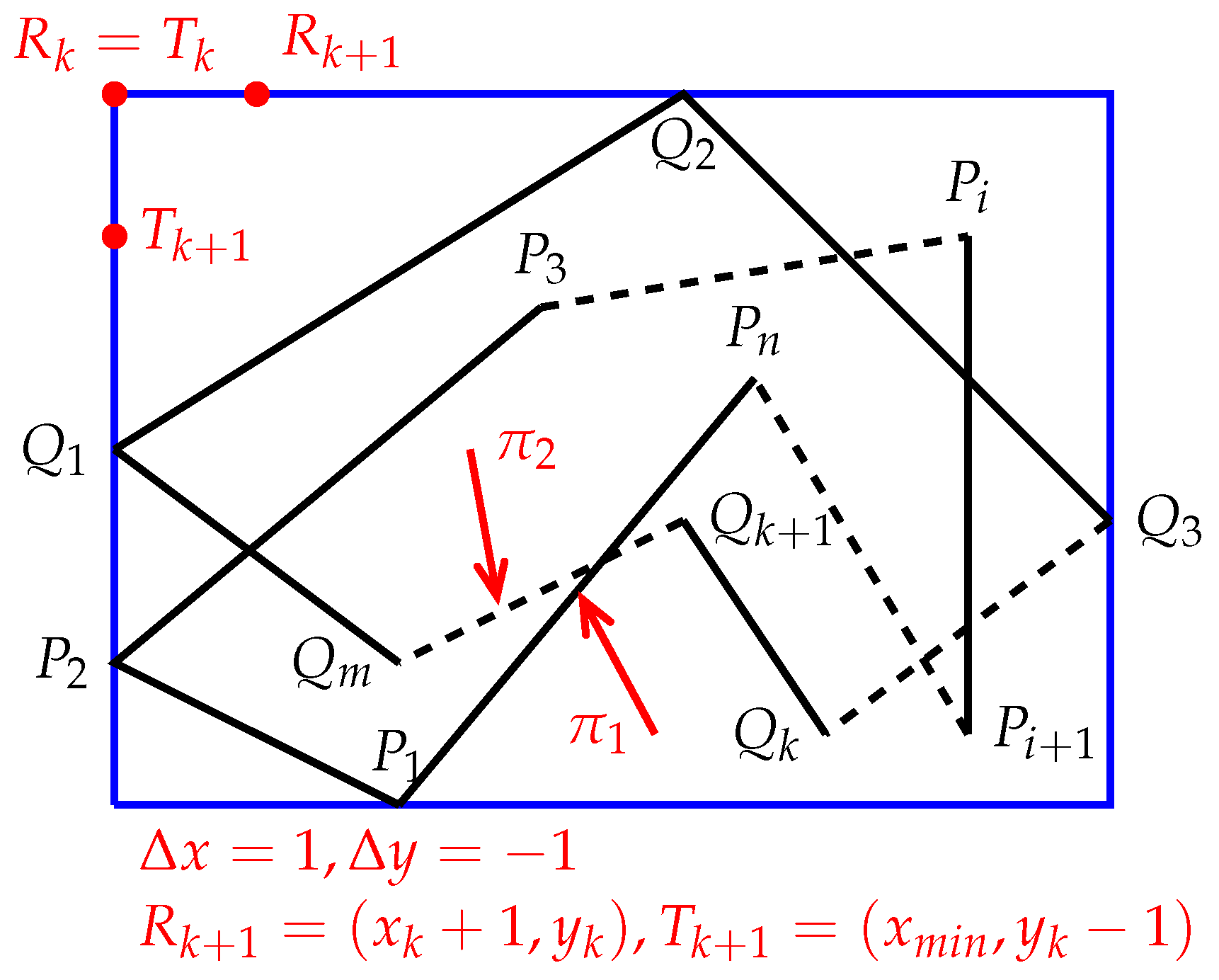
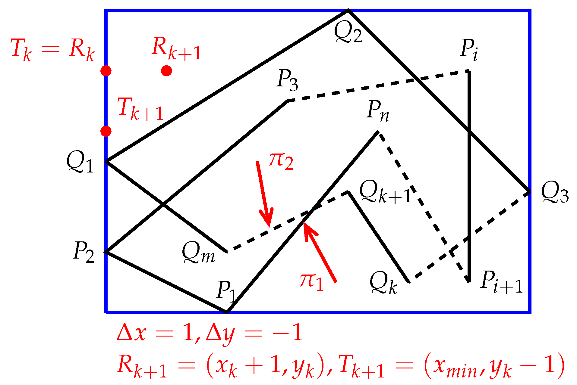
Using differential calculus, we will derive two iterative formulas by which Algorithm 2 can quickly determine the positional relationships between a set of points and a set of polygons. For this purpose, assume that Algorithm 2 sweeps across an intermediate point $R_k=(x_k,y_k)$ ($R_k\in MBB$ and see Figure 7), and the meaning of Q (below) is the same as the previous definition of Q. Suppose that Algorithm 2 already knows if $R_k=(x_k,y_k)$ is inside, outside, or on the boundary of S. Let $T_k=(x_{min},y_k)$($T_k\in MBB$ and see Figure 7), $R_{k+1}=(x_{k+1},y_{k+1})=(x_k+\Delta x,y_k)$, and $T_{k+1}=(x_{min},y_{k+1})=(x_{min},y_k+\Delta y)$ where $x_{min}$ is the smallest x-coordinate of the $MBB$. For the point $R_k$, the following situations may occur:

• $R_k$ is in the top-left corner of $MBB$ (see Figure 8).
• $R_k$ is on the left border of $MBB$ (see Figure 9).
• $R_k$ is inside the $MBB$ (see Figure 7).

Algorithm 2: Performing boolean operations on two polygons.

In Case 1, the equalities $R_k=T_k=(x_k,y_k)=(x_{min},y_{max})$ hold, where $x_{min}$ is the smallest x-coordinate of $MBB$ and $y_{max}$ is the largest y-coordinate of $MBB$. Thus, we have $R_{k+1}=(x_{k+1},y_{k+1})=(x_k+\Delta x,y_k)=(x_k+\Delta x,y_{max})$, $T_{k+1}=(x_{min}$, and $y_k+\Delta y)$.

In Case 2, the equalities $R_k=T_k=(x_k,y_k)=(x_{min},y_k)$ hold, where $x_{min}$ is the smallest x-coordinate of $MBB$. Therefore, we have $R_{k+1}=(x_{k+1},y_{k+1})=(x_k+\Delta x,y_k)=(x_{min}+\Delta x,y_k)$, $T_{k+1}=(x_{min}$, and $y_k+\Delta y)$.

In Case 3, with $R_k=(x_k,y_k)$, $T_k=(x_{min},y_k)$, the condition $R_k\ne T_k$ holds, where $x_{min}$ is the smallest x-coordinate of $MBB$. Therefore, we have $R_{k+1}=(x_{k+1},y_{k+1})=(x_k+\Delta x,y_k)$, $T_{k+1}=(x_{min}$, and $y_k+\Delta y)$.

In Figure 7, assume that $\Delta x=1$ and $\Delta y=-1$. Then, $R_{k+1}=(x_k+\Delta x,y_k)=(x_k+1,y_k)$ and $T_{k+1}=(x_{min},y_k+\Delta y)=(x_{min},y_k-1)$. If $R_k$ (P in Figure 2) is outside S and the variable k is 0, then $\overrightarrow{R_{k}Q}$ does not intersect $\overrightarrow{P_i{P}_{i+1}}$ for any $i=1,2,\cdots$, m. Thus, the positional relationships between $\overrightarrow{R_{k}Q}$ and $\overrightarrow{P_i{P}_{i+1}}$ belong to Cases 5–8, 11–15, or 22–26 (see Figure 2). Therefore, to determine the positional relationships between $\overrightarrow{R_{k+1}Q}$ and $\overrightarrow{P_i{P}_{i+1}}$ , Algorithm 2 only must recheck those edges whose positional relationships with $\overrightarrow{R_{k}Q}$ belong to Cases 5–8. Likewise, if $T_k$ (P in Figure 2) is outside S and the variable k is 0, to determine the positional relationships between $\overrightarrow{T_{k+1}Q}$ and $\overrightarrow{P_i{P}_{i+1}}$ , Algorithm 2 only must recheck those edges whose positional relationships with $\overrightarrow{T_{k}Q}$ belong to Cases 7–15.

If the variable k is even or odd, then the positional relationships between $\overrightarrow{R_{k}Q}$ ($R_k$ corresponds to P in Figure 2) and $\overrightarrow{P_i{P}_{i+1}}$ do not belong to Cases 1, 2, and 16–21. Therefore, to determine the positional relationships between $\overrightarrow{R_{k+1}Q}$ and $\overrightarrow{P_i{P}_{i+1}}$ , Algorithm 2 only must recheck those edges whose positional relationships with $\overrightarrow{R_{k}Q}$ belong to Cases 3–10. Likewise, if the variable k is even or odd, the positional relationships between $\overrightarrow{T_{k}Q}$ ($T_k$ corresponds to P in Figure 2) and $\overrightarrow{P_i{P}_{i+1}}$ do not belong to Cases 1, 2, and 16–21, to determine the positional relationships between $\overrightarrow{T_{k+1}Q}$ ($T_{k+1}$ corresponds to P in Figure 2) and $\overrightarrow{P_i{P}_{i+1}}$ , Algorithm 2 only must recheck those edges whose positional relationships with $\overrightarrow{T_{k}Q}$ belong to Cases 7–15.

If $R_k$ (P in Figure 2) is on the boundary of S, then the positional relationships between $\overrightarrow{R_{k}Q}$ and $\overrightarrow{P_i{P}_{i+1}}$ belong to Cases 1, 2, or 16–21. Therefore, to determine the positional relationships between $\overrightarrow{R_{k+1}Q}$ and $\overrightarrow{P_i{P}_{i+1}}$ , Algorithm 2 only must recheck those edges whose positional relationships with $\overrightarrow{R_{k}Q}$ belong to Case 1–10. Likewise, if $T_k$ (P in Figure 2) is on the boundary of S, to determine the positional relationships between $\overrightarrow{T_{k+1}Q}$ and $\overrightarrow{P_i{P}_{i+1}}$ , Algorithm 2 only must recheck those edges whose positional relationships with $\overrightarrow{T_{k}Q}$ belong to Cases 7–19.

From the above comparative analysis, it can be seen that to determine the positional relationship between $R_{k+1}$ and S, Algorithm 2 does not need to recheck all edges of S and usually needs only to recheck a small number of the edges whose number depends on the positional relationship between $R_{k+1}$ and S. Summarizing these findings, we get the following Theorem 2 by Definition 4.

Theorem 2.

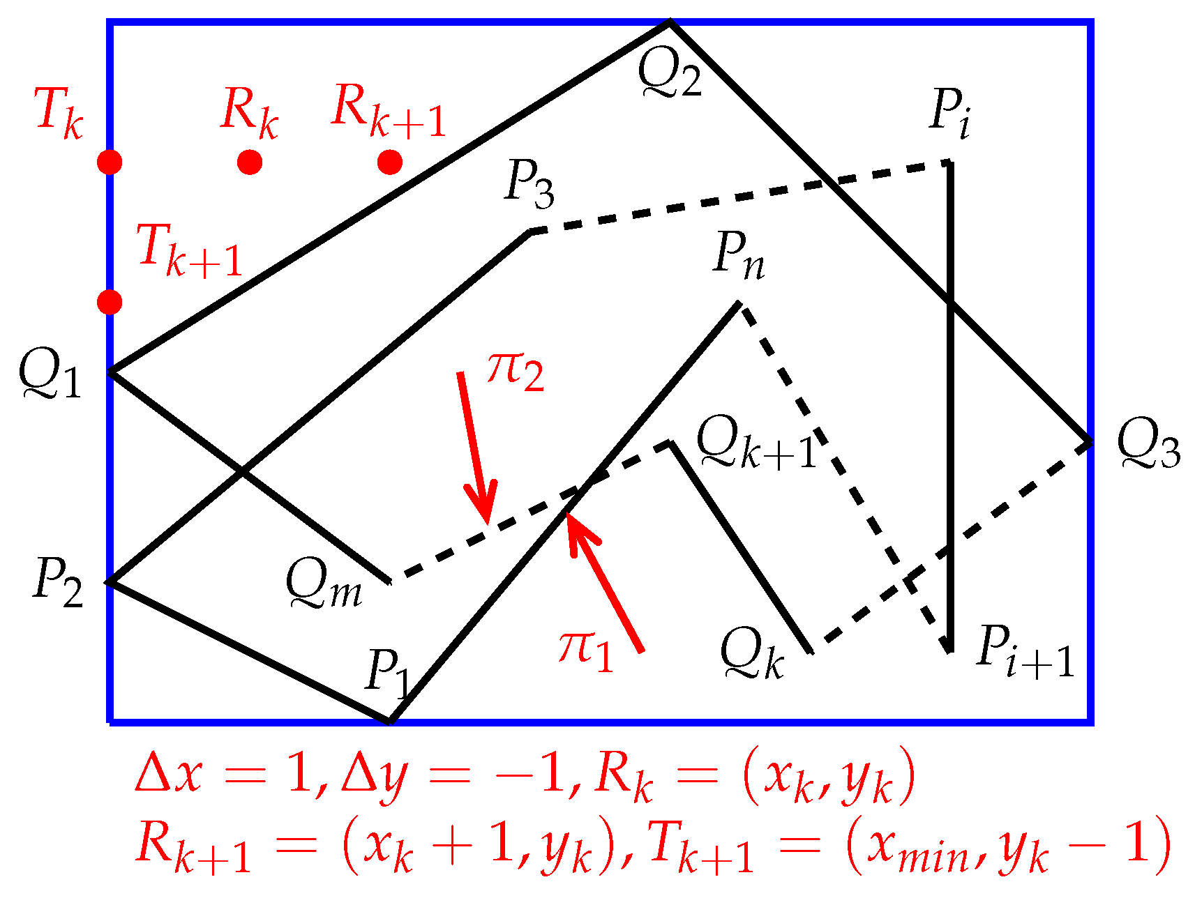
Suppose that $\pi 1$ and $\pi 2$ are two polygons. Assume that $MBB$ is the minimum bounding box of $\pi 1$ and $\pi 2$. Let $R_k=(x_k,y_k)$ be a point inside $MBB$ or on the boundary of $MBB$, and assume $T_k=(x_{min},y_k)$ is a point on the left border of $MBB$, where $x_{min}$ is the smallest x-coordinate of $MBB$ (see Figure 8). Let $R_{k+1}=(x_{k+1},y_{k+1})=(x_k+\Delta x,y_k)$ and $T_{k+1}=(x_{min}$, $y_{k+1})$ $=(x_{min},y_k+\Delta y)$. Let $S=\pi 1$ or $S=\pi 2$. Assume that $\Delta x=1$, and $\Delta y=-1$.

1.

If the odd-even number $S\left(R_k\right)=0$, to calculate $S\left(R_{k+1}\right)$ one needs only to recheck the edges of S belonging to Cases 5–8 (see Figure 2). Likewise, if the odd-even number $S\left(T_k\right)$ $=0$, to calculate $S\left(T_{k+1}\right)$, one needs only to recheck the edges of S belonging to Cases 7–15 (see Figure 2).

2.

If the odd-even number $S\left(R_k\right)$ is even or odd, to calculate $S\left(R_{k+1}\right)$ one needs only to recheck the edges of S belonging to Cases 3–10 (see Figure 2). Likewise, if the odd-even number $S\left(T_k\right)$ is even or odd, to calculate $S\left(T_{k+1}\right)$, one needs only to recheck the edges of S belonging to Cases 7–15 (see Figure 2).

3.

If the odd-even number $S\left(R_k\right)=-1$, to calculate $S\left(R_{k+1}\right)$, one needs only to recheck the edges of S belonging to Cases 1–10 (see Figure 2). Likewise, if the odd-even number $S\left(T_k\right)=-1$, to calculate $T\left(R_{k+1}\right)$, one needs only to recheck the edges of S belonging to Cases 7–19 (see Figure 2).

Proof. 

1. If the odd-even number $S\left(R_k\right)=0$, then $R_k$ (P in Figure 2) is outside S and $\overrightarrow{R_{k}Q}$ does not intersect $\overrightarrow{P_i{P}_{i+1}}$ for any $i=1,2,\cdots$, m. Thus, the positional relationships between $\overrightarrow{R_{k}Q}$ and $\overrightarrow{P_i{P}_{i+1}}$ only belong to Cases 5–8, 11–15, or 22–26 (see Figure 2). Therefore, to determine the positional relationships between $\overrightarrow{R_{k+1}Q}$ and $\overrightarrow{P_i{P}_{i+1}}$ for calculating $S\left(R_{k+1}\right)$, one needs only to recheck the edges of S belonging to Cases 5–8 (see Figure 2). Likewise, if the odd-even number $S\left(T_k\right)$ $=0$, then $T_k$ (P in Figure 2) is outside S. Thus, the positional relationships between $\overrightarrow{T_{k}Q}$ and $\overrightarrow{P_i{P}_{i+1}}$ only belong to Cases 5–8, 11–15, or 22–26. Therefore, to determine the positional relationships between $\overrightarrow{T_{k+1}Q}$ and $\overrightarrow{P_i{P}_{i+1}}$ for calculatint $S\left(T_{k+1}\right)$, one needs only to recheck the edges of S belonging to Cases 7–15 (see Figure 2).

2. If the odd-even number $S\left(R_k\right)$ is even or odd, then the positional relationships between $\overrightarrow{R_{k}Q}$ ($R_k$ corresponds to P in Figure 2) and $\overrightarrow{P_i{P}_{i+1}}$ do not belong to Cases 1, 2, and 16–21. Therefore, to determine the positional relationships between $\overrightarrow{R_{k+1}Q}$ and $\overrightarrow{P_i{P}_{i+1}}$ for calculating $S\left(R_{k+1}\right)$, one needs only to recheck the edges of S belonging to Cases 3–10 (see Figure 2). Likewise, if the odd-even number $S\left(T_k\right)$ is even or odd, then the positional relationships between $\overrightarrow{T_{k}Q}$ ($T_k$ corresponds to P in Figure 2) and $\overrightarrow{P_i{P}_{i+1}}$ also do not belong to Cases 1, 2, and 16–21. Therefore, to determine the positional relationships between $\overrightarrow{T_{k+1}Q}$ ($T_{k+1}$ corresponds to P in Figure 2) and $\overrightarrow{P_i{P}_{i+1}}$ for calculating $S\left(T_{k+1}\right)$, one needs only to recheck the edges of S belonging to Cases 7–15 (see Figure 2).

3. If the odd-even number $S\left(R_k\right)=-1$, then $R_k$ (P in Figure 2) is on the boundary of S, then the positional relationships between $\overrightarrow{R_{k}Q}$ and $\overrightarrow{P_i{P}_{i+1}}$ only belong to Cases 1, 2, or 16–21. Therefore, to determine the positional relationships between $\overrightarrow{R_{k+1}Q}$ and $\overrightarrow{P_i{P}_{i+1}}$ for calculating $S\left(R_{k+1}\right)$, one needs only to recheck the edges of S belonging to Cases 1–10 (see Figure 2). Likewise, if the odd-even number $S\left(T_k\right)=-1$, then $T_k$ (P in Figure 2) is on the boundary of S. Thus, the positional relationships between $\overrightarrow{T_{k}Q}$ and $\overrightarrow{P_i{P}_{i+1}}$ only belong to Cases 1, 2, or 16–21. Therefore, to determine the positional relationships between $\overrightarrow{T_{k+1}Q}$ and $\overrightarrow{P_i{P}_{i+1}}$ for calculating $T\left(R_{k+1}\right)$, one needs only to recheck the edges of S belonging to Cases 7–19 (see Figure 2). □

Theorem 3.

Suppose that $\pi 1$ and $\pi 2$ are two polygons. Assume that $MBB$ is the minimum bounding box of $\pi 1$ and $\pi 2$. Let $R_k=(x_k,y_k)$ be a point inside or on the edges of $MBB$, and $T_k=(x_{min},y_k)$ is a point on the left border of $MBB$, where $x_{min}$ is the smallest x-coordinate of $MBB$. Let $R_{k+1}=(x_{k+1},y_{k+1})=(x_k+\Delta x,y_k)$ and $T_{k+1}=(x_{min},y_{k+1})=(x_{min},y_k+\Delta y)$ (see Figure 7, Figure 8 and Figure 9). Let $S=\pi 1$ or $S=\pi 2$. Suppose that $\overline{P_i{P}_{i+1}}$ is an edge of $S=\pi 1$ or $S=\pi 2$ with $P_i=(x_i,y_i)$ and $P_{i+1}=(x_{i+1},y_{i+1})$. Assume that $\Delta x=1$ and $\Delta y=-1$. If $F\left(R_k\right)$ and $F\left(T_k\right)$ satisfy Equation (1), then the following two iterative formulas hold.

$$\begin{array}{ccc}\hfill F\left(R_{k+1}\right)& =& F\left(R_k\right)+(y_i-y_{i+1}).\hfill \end{array}$$

(4)

$$\begin{array}{ccc}\hfill F\left(T_{k+1}\right)& =& F\left(T_k\right)+(x_i-x_{i+1}).\hfill \end{array}$$

(5)

By Equations (4) and (5), if Algorithm 2 already knows $F\left(R_K\right)$ and $F\left(T_K\right)$, Algorithm 2 can quickly calculate $F\left(R_{k+1}\right)$ and $F\left(T_{k+1}\right)$. Therefore, using Equations (4) and (5), one can simplify the calculation and improve processing speed significantly.

By Theorems 2 and 3, and Algorithm 1, vertex by vertex, Algorithm 2 determines the positional relationship between $R_k$ and ${\pi }_1$, yet between $R_k$ and ${\pi }_2$. Furthermore, according to the types of boolean operations, if $R_k$ is simultaneously inside ${\pi }_1$ and ${\pi }_2$ (also including on their border), then $R_k\in ({\pi }_1\cap {\pi }_2)$. Otherwise, if $R_k$ is inside ${\pi }_1$ or ${\pi }_2$ (also including on their border), then $R_k\in ({\pi }_1\cup {\pi }_2)$. Otherwise, if $R_k$ is both inside ${\pi }_1$(also including on its border) and outside ${\pi }_2$, then $R_k\in ({\pi }_1-{\pi }_2)$. Otherwise, if $R_k$ is both outside ${\pi }_1$ and inside ${\pi }_2$ (also including on their border), then $R_k\in ({\pi }_2-{\pi }_1)$. Step-by-step, Algorithm 2 is well able to complete the corresponding boolean operations. Algorithm 2 is a comprehensive presentation and summary for all preceding discussion.

Proof. 

By Equation (1), for $R_{k+1}$ and $T_{k+1}$ we have

$$\begin{array}{c}F\left(R_{k+1}\right)=F(x_{k+1},y_{k+1})=F(x_k+1,y_k)\hfill \\ =(y_i-y_{i+1})(x_k+1)+(x_{i+1}-x_i)y_k+x_i{y}_{i+1}-x_{i+1}{y}_i\hfill \\ =(y_i-y_{i+1})x_k+(x_{i+1}-x_i)y_k+x_i{y}_{i+1}-x_{i+1}{y}_i+(y_i-y_{i+1})\hfill \\ =F\left(R_k\right)+(y_i-y_{i+1}).\hfill \end{array}$$

$$\begin{array}{c}F\left(T_{k+1}\right)=F(x_{k+1},y_{k+1})=F(x_{min},y_{k+1})=F(x_{min},y_k-1)\hfill \\ =(y_i-y_{i+1})x_{min}+(x_{i+1}-x_i)(y_k-1)+x_i{y}_{i+1}-x_{i+1}{y}_i\hfill \\ =(y_i-y_{i+1})x_{min}+(x_{i+1}-x_i)y_k+x_i{y}_{i+1}-x_{i+1}{y}_i-(x_{i+1}-x_i)\hfill \\ =F\left(T_k\right)+(x_i-x_{i+1}).\hfill \end{array}$$

□

6. Complexity Analysis of Algorithms

In this section, we analyze the time and space complexities of our algorithms. First, let us consider Algorithm 1. Assume that the number of edges of a polygon is n. The for-loop in Steps 3–30 determines the positional relationship between point P and the n edge vectors $\overrightarrow{P_i{P}_{i+1}}$ with $i=1,2,\cdots ,n$. Steps 4 and 7 each perform two subtractions. One subtraction and two multiplication calculations are performed in function f in Steps 9, 15, 21, and 24. Step 5 performs at most seven operations, including four comparison operations and three logical operations. Steps 8, 14, 20, 23, 26, 27, and 29 each perform at most two comparison operations and one logical operation.

In the worst case, the for-loop must perform Steps 4–7, 8, 14, 20, 23, 26, 27, 29, and 30 simultaneously. Thus, the number of operations in the for-loop is equal to $2+7+2+3\times 7+1$ $=33$. Therefore, the total number of operations required is $33n+11$. Conversely, in the best case, the point P is on $\partial S$, and the for-loop must only perform Steps 4–10, 12, and 13 one time. As a result, the number of operations required is $7+2+7+2+3+3+3=27$.

Furthermore, let us compute the average running time of Algorithm 1. Algorithm 1 includes many branch statements whose execution probabilities are all different. From the previous discussions, we know that the probability of a point lying on the boundary is far less than the probability of the point not lying on the boundary. Therefore, to calculate the average running time required by Algorithm 1, we only must consider the case in which the point is not on $\partial S$. Furthermore, we only must consider the paths that the for-loop most likely performs, 4→5→6, 4→5→7→8→9→10→11, or 4→5→7→8→14→15→16→17.

For an edge, the average number of operations required is

$$(1/3)\times (3\times 2+3\times 7+2\times 2+3\times 2+2\times 3+2\times 1+3+2)$$

$$=(1/3)\times \left(50\right)=(50/3)=16.7.$$

Because the number of polygon edges is n, the total average number of operations required is $16.7n$ for Steps 3–30. Steps 31–32 require at most two logical operations, and one modulo operation. Therefore, the total average number of operations required is $16.7n+3$. Because Algorithm 1 uses an array to store the edge information, including the end nodes of each edge, its space complexity is also $O\left(n\right)$. The time and space complexities of Algorithm 1 are the same as Algorithm 1.

Second, let us consider Algorithm 2. Assume that the numbers of edges of two input polygons are $n,m$ respectively. In addition, assume that execution probability of each branch is different for the for-loop in Algorithm 1. Step 5 requires at most 4$(n+m)$ operations. For R, on average, Step 10 requires $16.7(n+m)+6$ operations. Step 11 requires at most three operations. In the worst case, Steps 12–44 require at most $10+4(n+m)$ operations. Therefore, in the worst case, the time complexity of Algorithm 2 is $O\left(\right(n+m\left)l\right)$, where

$$\begin{array}{c}\hfill l=(Bottom\_Right.x-Top\_Left.x)\times (Top\_Left.y-Bottom\_Right.y).\end{array}$$

(6)

Under normal circumstances, because the numbers of operations for Steps 10 and 12–44 are far less than $16.7(n+m)+6$ and $10+4(n+m)$, the average time complexity of Algorithm 2 is far less than $O\left(\right(n+m\left)l\right)$. No matter how complex the input polygons are, it can be seen that l is nearly constant. Thus, Algorithm 2 has an average time complexity of $O(n+m)$, reconfirmed through the experimental results in Section 7.

7. Experiment and Comparison

We have completed experimental tests to evaluate the performances of Algorithms 1 and 2. Our computing environment used an Intel(R) Core(TM)2 Quad CPU Q6600 @2.40 GHz with 4.00 GB of RAM. The operating system is Microsoft Windows 10 Professional Edition. The graphics card is an NVIDIA GeForce 9800 GT. The display resolution is $1024\times 768\times 32$ bits (RGB). The internal hard drive is 1TB. We used Microsoft Visual C++ 2017 compiler as our programming environment. The testing program randomly generates vertices of a polygon using the methodology in [31].

7.1. The Point-in-Polygon Test

From the online library [5], we select 11 algorithms for testing. In addition, we test [1,6] and efficient boundary methods [2], and CGAL4.2 [31] with a 2D Kernel. Thus, the algorithms tested include a total of 16 algorithms (see

Table 1. Performance comparison of the different algorithms for the point-in-polygon test. CROSS indicates that an algorithm can handle self-intersecting polygons. HOLE denotes that an algorithm can deal with polygons with holes(not nested). NHOLE denotes that an algorithm can deal with polygons with nested holes at any depth. KHOLE denotes that an algorithm can deal with polygons with keyhole edges formed by single contours. DIR indicates that an algorithm must specify whether each contour of input polygons is oriented clockwise or counterclockwise. SENS indicates that an algorithm is sensitive to whether a polygon is oriented clockwise or counterclockwise. ON indicates that an algorithm can determine whether a point is on the polygon boundary. BUG denotes that an algorithm has bugs.

		Properties	CROSS	HOLE	NHOLE	KHOLE	DIR	SENS	ON	BUG
	Result
Library
1	Algorithm 1		✓	✓	✓	✓	✗	✗	✓	✗
2	Crossings		✗	✓	✗	✗	✗	✗	✗	✗
3	Crossings-multiply [4,5]		✓	✓	✗	✓	✗	✗	✗	✗
4	Angle summation		✓	✓	✗	✓	✗	✗	✗	✗
5	Weiler angle summation		✗	✓	✗	✗	✗	✗	✗	✗
6	Half-plane testing		✓	✓	✗	✓	✗	✗	✗	✓
7	Barycentric coordinates		✓	✓	✗	✓	✗	✗	✗	✓
8	Spackman barycentric		✓	✓	✗	✓	✗	✗	✗	✓
9	Trapezoid testing		✗	✓	✗	✗	✗	✗	✗	✓
10	Grid testing		✓	✓	✗	✓	✗	✗	✗	✓
11	Exterior test		✗	✓	✗	✗	✗	✗	✗	✗
12	Inclusion test		✗	✓	✗	✗	✗	✗	✗	✗
13	Jiménez et al. [1]		✗	✓	✗	✗	✓	✓	✗	✓
14	Galacticomm [6]		✓	✓	✗	✓	✗	✗	✗	✗
15	Efficient boundary [2]		✗	✗	✗	✗	✓	✓	✗	✓
16	CGAL4.2 [31]		✓	✓	✓	✓	✗	✗	✓	✗

).

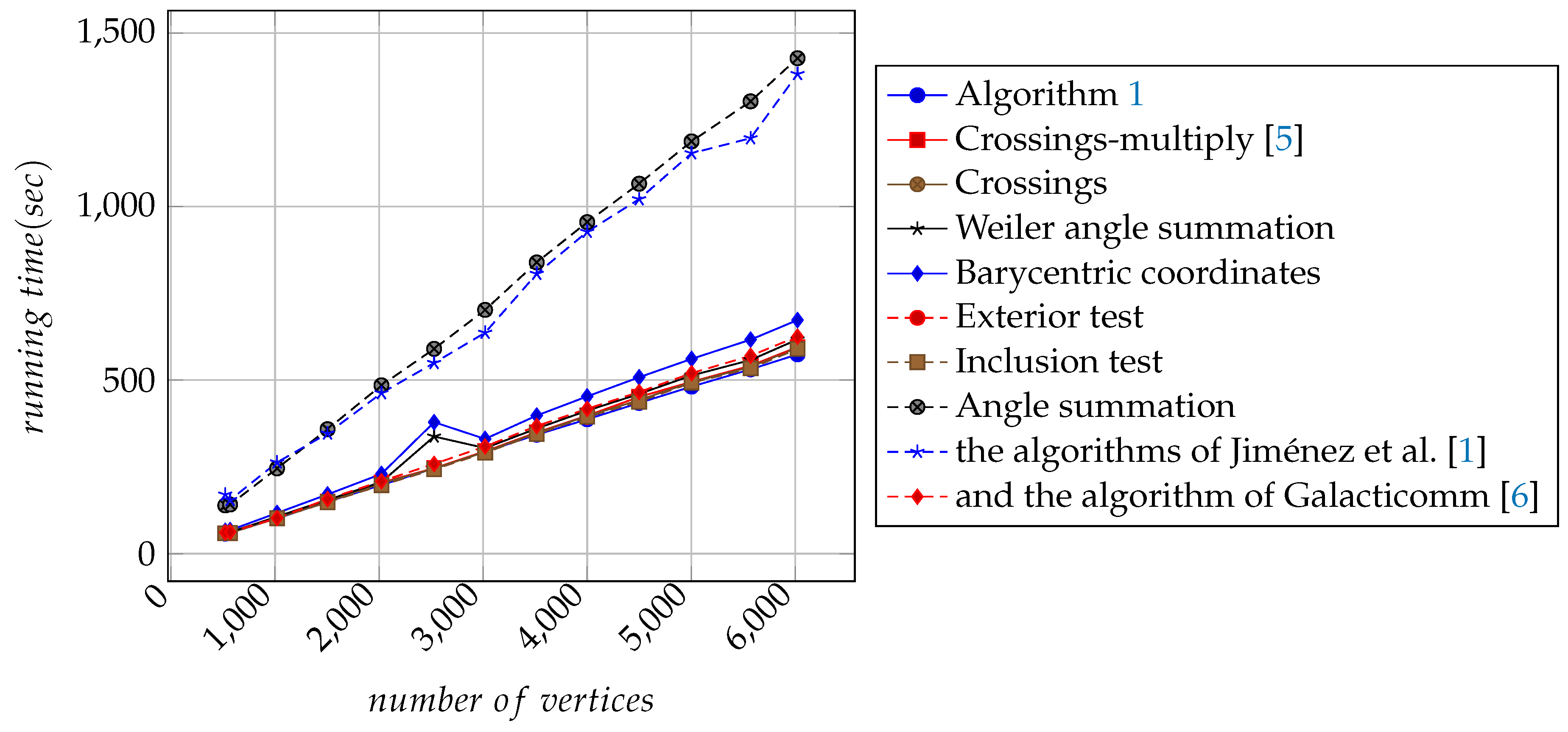
Figure 10 shows the performance comparison of the 10 algorithms in running time. We can see that, although the running times of the 10 algorithms changed almost linearly as the number of vertices of input polygons increase, Algorithm 1 increases more slowly than the other algorithms. From the top-left corner to the bottom-right corner of the $MBB$, the testing program determines point-by-point whether a point is inside, outside, or on the boundary of the polygons. For all points in the $MBB$, the algorithm tested uses a timer to record the total execution time of the program. Finally, the results of the executions were used to plot the curves with the $number$ $of$ $vertices=$ 522, 569, 1020, 1505, 2023, 2529, 3019, 3515, 4000, 4499, 5003, 5570, and 6021 (see Figure 10). The x-axis denotes the number of vertices of an input polygon and the y-axis denotes the running time of an algorithm in seconds (same as below) as shown in Figure 10. Because the implementations of half-plane testing, Spackman barycentric, Trapezoid testing, Grid testing, and Efficient boundary [2] all contain bugs, we do not plot their corresponding graphs.

Half-plane testing, Barycentric coordinates, and Spackman barycentric algorithms sometimes misjudge internal points as external points (see Figure 1). To store the number of trapezoids, the implementation of Trapezoid algorithm uses the global variable Trapezoid_Bins that has initial value 20. The performance of Trapezoid algorithm changes as the value of the variable Trapezoid_Bins changes. To keep the value of resolution, the implementation of Grid testing algorithm uses the global variable Grid_Resolution that has initial value 20. The performance of Grid testing algorithm changes as Grid_Resolution changes. According to the resolution of the screen, Grid testing algorithm partitions the bounding box into grids, the number of which varies as the screen resolution varies. Grid testing consumes more memory and time to the extent that it frequently causes the program to crash. Jiménez et al. [1] were sensitive to whether a polygon is clockwise or counterclockwise oriented and do not apply to a self-intersecting polygons (see Figure 1). In addition, it cannot efficiently deal with degenerate cases.

From the comparison results, it can be seen that, although Algorithm 1 uses many comparison operations of floating-point numbers, this does not cause the program to run incorrectly. Performance of Algorithm 1 is only subject to the number of vertices of tested polygon, rather than the number of floating point operations involved. Therefore, introducing errors $ϵ$ for comparison operation of floating point numbers is not essential for Algorithm 1. Of course, if people want “fat edges”, they can enlarge the bounds by an epsilon.

7.2. Boolean Operations Test

From the online library, we selected three algorithms for testing of boolean operations. Thus, the comparison includes a total of four algorithms (see

Table 2. Performance comparison of the different algorithms for boolean operations. The meanings of symbols below are the same as those in Table 1.

		Properties	CROSS	HOLE	NHOLE	KHOLE	DIR	SENS	BUG
	Result
Library
1	Algorithm 2		✓	✓	✓	✓	✗	✗	✗
2	CGAL4.2 [31]		✗	✓	✗	✗	✓	✓	✓
3	GPC [32]		✓	✓	✓	✓	✗	✗	✗
4	Clipper4.6.3 [33]		✓	✓	✓	✓	✗	✗	✗

).

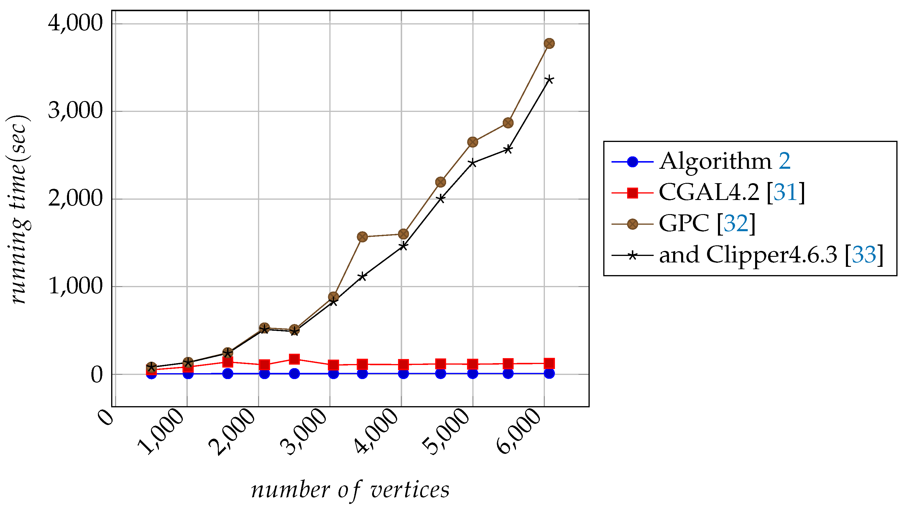
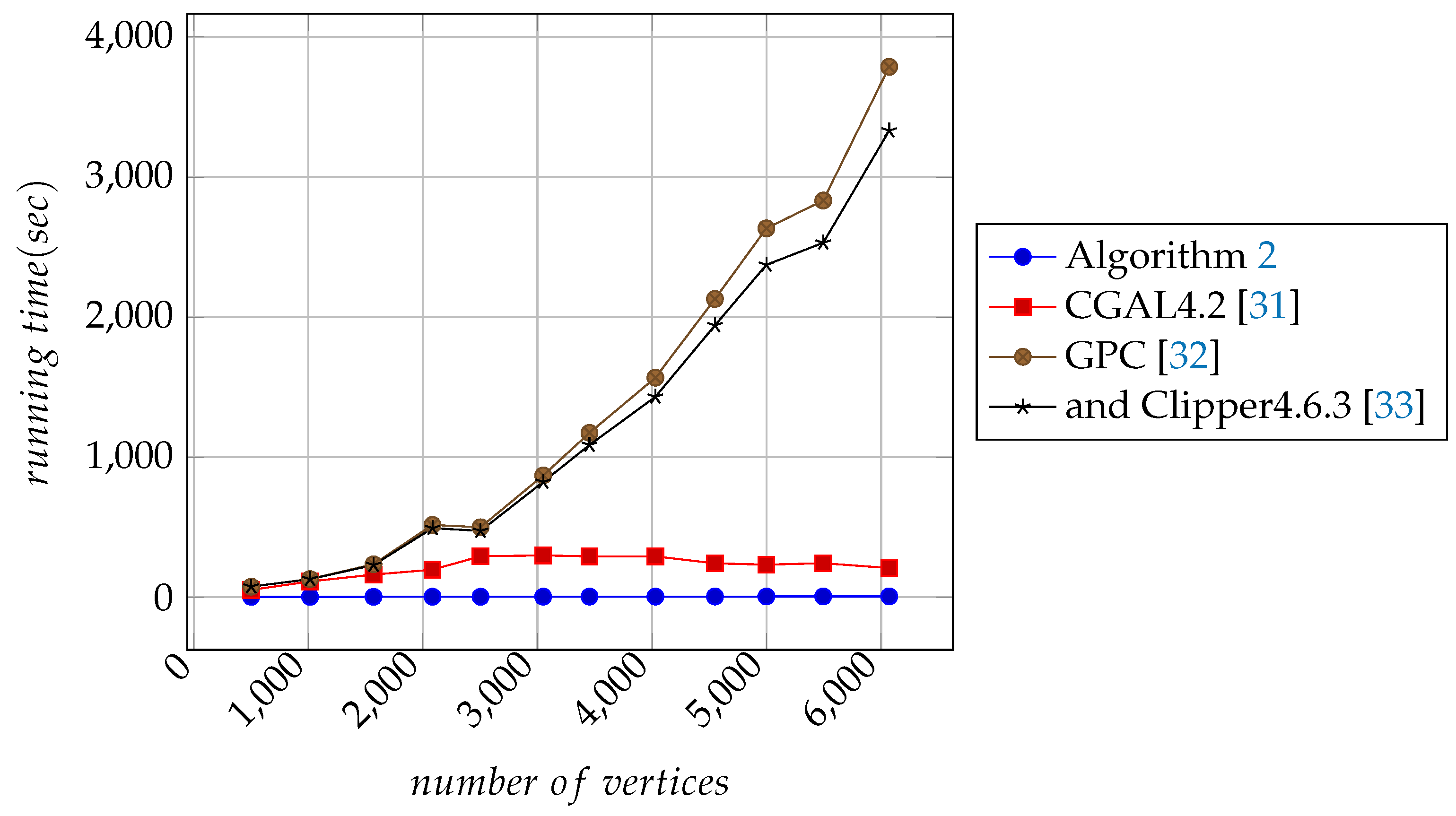
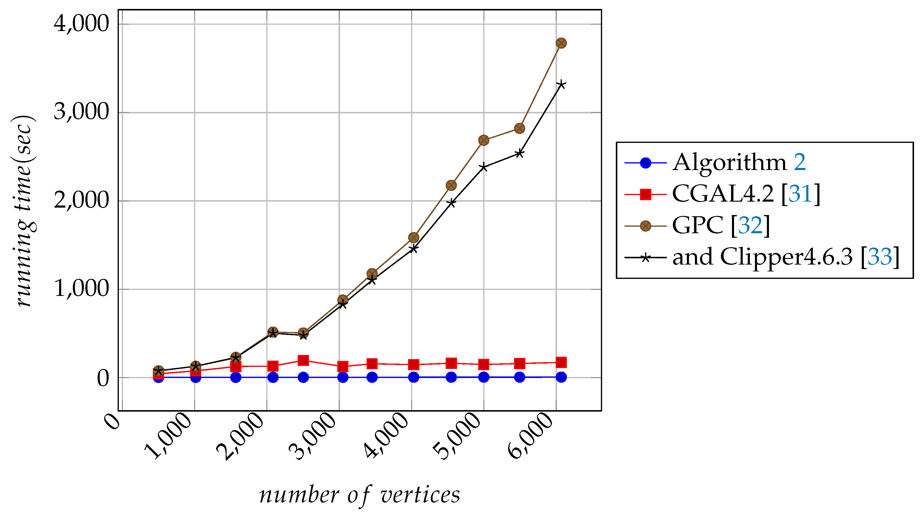
All algorithms except Algorithm 2 perform boolean operations to generate the corresponding resultant polygons. They then use crossings-multiplication [4,5] to fill the interior regions of the resultant polygons. For the input polygons, Algorithm 2 takes only a calculation step to fill the interior regions of the resultant polygons. For measuring the running times of the algorithms, each algorithm uses a timer to record the total execution time. Finally, based on the results of the operations, we plot the curves with $number$ $of$ $vertices=$ 501, 1015, 1569, 2084, 2503, 3050, 3454, 4029, 4549, 4998, 5494, and 6070 in Figure 11, Figure 12 and Figure 13.

It is clear in Figure 11, Figure 12 and Figure 13 that the execution time of Algorithm 2 is minimal and approximately proportional to the number of vertices in input polygons. It can be seen in Table 2 that Algorithm 2, GPC [32], and Clipper4.6.3 [33] all have excellent performance under the same test conditions.

8. Results and Discussion

In Figure 10, it can be seen that, with the increase of the number of vertices, the computation time of Algorithm 1 is getting less and less than the computational time of any other algorithm needed for the point-in-polygon test. This means that, with the increase of the number of points, the processing speed of Algorithm 1 is faster than any other algorithm.

Theorem 4.

Let S be a closed polygon. The performance of Algorithm 1 is optimal for the point-in-polygon test on S.

Proof. 

By Section 6, it follows that, because the total average number of operations required is $16.7n+3$, the time complexity of Algorithm 1 is $O\left(n\right)$ where n is the number of polygon edges. Clearly, the space complexity of Algorithm 1 is also $O\left(n\right)$.

In Figure 10, it can be seen that the run time of Algorithm 1 for the point-in-polygon test is minimal. Therefore, the computational performances of Algorithm 1 is better than that of the other algorithms. Observe that the related performances of Algorithms 1 described in Table 1 go beyond that of the other algorithms except CGAL4.2 [31].

Although the time and space complexities of Algorithm 1 are the same as the state-of-the-art methods for the point-in-polygon test, Algorithm 1 is optimal. Further, we present the following facts to support our view:

• It handles all degenerate cases and simultaneously provides a corresponding solution to each degenerate case (see Figure 2). These tactics both ensure its robustness and creates the prerequisites and basis for Algorithm 2.
• It uses Equation (3) to reduce the running time.
• It uses the Jordan property of a vector to determine the positional relationship between a point and an edge, which avoids computing the intersection point and division operations.
• It involves only addition, subtraction, multiplication, comparison, and logical operations such that it is unnecessary to compute any angle. In addition, It eliminates other time-consuming operations such as preprocessing.
• It does not impose any restrictions on the shape of input polygons, and is applicable to any polygons, including self-intersecting polygons or polygons with holes nested to any level of depth (see Figure 3a). Therefore, It can both quickly determine whether a point is inside or outside a polygon and accurately determine the contours of input polygon (see Figure 3b).
• It does not need to sort the vertices clockwise or counterclockwise beforehand. Therefore, it processes all edges one by one in any order for each input polygon.
• It is parallelizable because its many operations can be done in parallel.
• A detailed theoretical analysis and the proof of the correctness of Algorithm 1 (see Theorems 1) for the point-in-polygon test are shown.
• It considers the execution probability of each conditional branch and uses these probabilities to optimize the program flow.

Therefore, it follows that the conclusion of Theorem 4 holds. □

Although the comparison operations of floating point numbers introduced in Algorithm 1 increase the running time of the program and reduce its computing speed, the speed reduction is limited and would not cause the program significantly reduced operating speed. Although Algorithm 1 uses many comparison operations of floating-point numbers, this does not cause the program to run incorrectly. Performance of Algorithm 1 is only subjected to the number of vertices of tested polygon, rather than the number of floating point operations involved.

Based on Algorithm 1, Algorithm 2 inherits all of its advantages, including the simple data structure, low running time, high stability, and reliability. Algorithm 2 assigns each vector $\overrightarrow{P_i{P}_{i+1}}$ in Figure 2a–z a number code corresponding to Cases 1–26. In addition, Algorithm 2 uses two iterative formulas (Equations (4) and (5)) to calculate $F\left(R\right)$ and $F\left(T\right)$. Results from experiments show that the use of the two strategies increase processing speed and can accurately solve the given problem.

Our method can be applied to 3D printing [8] to improve the 3D printing performance. The mechanism that we conceive for 3D printing is as follows: When performing 3D printing, we first use the planes $z=z_0,z=z_0+1,\cdots ,z=z_0+n$ to intercept object in the size of the z-axis from small to large, and then we apply Algorithm 2 on the plane $z=z_0,z=z_0+1,\cdots ,z=z_0+n$. This will enable 3D printing.

9. Conclusions and Future Works

In summary, we draw the following conclusions. Algorithm 1 with time complexity $O\left(n\right)$, is optimal for the point-in-polygon test. Algorithm 2, with worst case time complexity $O\left(\right(n+m\left)l\right)$, is a novel algorithm for boolean operations. Algorithms 1 and 2 are stable and reliable and can be extended to three-dimensional space. In particular, our method can be applied to 3D printing to improve the 3D printing performance.

We will explore how to extend Algorithms 1 and 2 into 3D space and how to improve reliability and efficiency of the point-in-polyhedral test and boolean operations on 3D objects. We will discuss and show how to solve the related problems in other articles.

References

- Jiménez, J.J.; Feito, F.R.; Segura, R.J. Robust and Optimized Algorithms for the Point-in-Polygon Inclusion Test without Pre-processing. Comput. Graph. Forum 2009, 28, 2264–2274. [Google Scholar] [CrossRef]
- Hormann, K.; Agathos, A. The point in polygon problem for arbitrary polygons. Comput. Geom. 2001, 20, 131–144. [Google Scholar] [CrossRef]
- DonaldHearn. Computer Graphics C Version; Prentice Hall: Upper Saddle River, NJ, USA, 1997. [Google Scholar]
- Haines, E. Point in polygon strategies. Graph. Gems IV 1994, 994, 24–46. [Google Scholar]
- Haines, E. Graphics Gems Repository. Available online: http://0-tog-acm-org.brum.beds.ac.uk/resources/GraphicsGems/ (accessed on 7 August 2018).
- Galacticomm. A Point about Polygons (Article in 3/97 Linux Journal). Available online: http://www.visibone.com/inpoly/ (accessed on 7 August 2018).
- Weiler, K. Polygon comparison using a graph representation. SIGGRAPH Comput. Graph. 1980, 14, 10–18. [Google Scholar] [CrossRef]
- Hoy, M.B. 3D Printing: Making Things at the Library. Med. Ref. Serv. Q. 2013, 32, 93–99. [Google Scholar] [CrossRef] [PubMed]
- Nievergelt, J.; Preparata, F.P. Plane-sweep algorithms for intersecting geometric figures. Commun. ACM 1982, 25, 739–747. [Google Scholar] [CrossRef] [Green Version]
- Galetzka, M.; Glauner, P.O. A correct even-odd algorithm for the point-in-polygon (PIP) problem for complex polygons. arXiv, 2012; arXiv:1207.3502. [Google Scholar]
- Wang, W.; Li, J.; Wu, E. 2D point-in-polygon test by classifying edges into layers. Comput. Graph. 2005, 29, 427–439. [Google Scholar] [CrossRef]
- Sederberg, T.W.; Nishita, T. Curve intersection using Bézier clipping. Comput. Aided Des. 1990, 22, 538–549. [Google Scholar] [CrossRef]
- Bartoň, M.; Jüttler, B. Computing roots of polynomials by quadratic clipping. Comput. Aided Geom. Des. 2007, 24, 125–141. [Google Scholar] [CrossRef]
- Aizenshtein, M.; Bartoň, M.; Elber, G. Global solutions of well-constrained transcendental systems using expression trees and a single solution test. Comput. Aided Geom. Des. 2012, 29, 265–279. [Google Scholar] [CrossRef]
- Van Sosin, B.; Elber, G. Solving piecewise polynomial constraint systems with decomposition and a subdivision-based solver. Comput. Aided Des. 2017, 90, 37–47. [Google Scholar] [CrossRef]
- Gombos˘i, M.; Žalik, B. Point-in-polygon tests for geometric buffers. Comput. Geosci. 2005, 31, 1201–1212. [Google Scholar] [CrossRef]
- Yang, S.; Yong, J.H.; Sun, J.; Gu, H.; Paul, J.C. A point-in-polygon method based on a quasi-closest point. Comput. Geosci. 2010, 36, 205–213. [Google Scholar] [CrossRef] [Green Version]
- Lorenzetto, G.P.; Datta, A.; Thomas, R.C. A fast trapezoidation technique for planar polygons. Comput. Graph. 2002, 26, 281–289. [Google Scholar] [CrossRef] [Green Version]
- Martínez, F.; Rueda, A.J.; Feito, F.R. The multi-L-REP decomposition and its application to a point-in-polygon inclusion test. Comput. Graph. 2006, 30, 947–958. [Google Scholar] [CrossRef]
- Rueda, A.J.; Feito, F.R. EL-REP: A New 2D Geometric Decomposition Scheme and Its Applications. IEEE Trans. Vis. Comput. Graph. 2011, 17, 1325–1336. [Google Scholar] [CrossRef] [PubMed]
- Andreev, R.D. Algorithm for Clpping Arbitrary Polygons. Comput. Graph. Forum 1989, 8, 183–191. [Google Scholar] [CrossRef]
- Rappoport, A. An efficient algorithm for line and polygon clipping. Vis. Comput. 1991, 7, 19–28. [Google Scholar] [CrossRef]
- Greiner, G.; Hormann, K. Efficient clipping of arbitrary polygons. ACM Trans. Graph. 1998, 17, 71–83. [Google Scholar] [CrossRef]
- Weiler, K.; Atherton, P. Hidden surface removal using polygon area sorting. SIGGRAPH Comput. Graph. 1977, 11, 214–222. [Google Scholar] [CrossRef]
- Vatti, B.R. A generic solution to polygon clipping. Commun. ACM 1992, 35, 56–63. [Google Scholar] [CrossRef]
- Martínez, F.; Rueda, A.J.; Feito, F.R. A new algorithm for computing Boolean operations on polygons. Comput. Geosci. 2009, 35, 1177–1185. [Google Scholar] [CrossRef]
- Feito, F.R.; Rivero, M. Geometric modelling based on simplicial chains. Comput. Graph. 1998, 22, 611–619. [Google Scholar] [CrossRef]
- Rivero, M.; Feito, F.R. Boolean operations on general planar polygons. Comput. Graph. 2000, 24, 881–896. [Google Scholar] [CrossRef]
- Peng, Y.; Yong, J.H.; Dong, W.M.; Zhang, H.; Sun, J.G. A new algorithm for Boolean operations on general polygons. Comput. Graph. 2005, 29, 57–70. [Google Scholar] [CrossRef] [Green Version]
- Graysmith, J.; Shaw, C. Automated procedures for Boolean operations on finite element meshes. Eng. Comput. 1997, 14, 702–717. [Google Scholar] [CrossRef]
- CGAL4.2. CGAL—Computational Geometry Algorithms Library. Available online: http://www.cgal.org/ (accessed on 7 August 2018).
- GPC, A.M. GPC General Polygon Clipper Library from The University of Manchester. Available online: http://www.cs.man.ac.uk/toby/alan/software/ (accessed on 7 August 2018).
- Clipper4.6.3. Clipper—An Open Source Freeware Polygon Clipping Library. Available online: http://www.angusj.com/delphi/clipper.php (accessed on 7 August 2018).
Figure 1.
A comparison of several algorithms for the point-in-polygon test. Apart from (b), the remaining tests, including (c–g), all contain bugs that can be observed by enlarging them: (a) the initial contour; (b) using Algorithm 1; (c) using the algorithms of Jiménez et al. [1]; (d) using Half-plane testing; (e) using Barycentric coordinates; (f) using Spackman barycentric; and (g) using Efficient boundary [2].
Figure 2.
A detailed description of the 26 kinds of positional relationships existing between and , and the corresponding processing results. Here, k is the variable to accumulate the total number of intersections made by and all edges of S: (a) P is on ; (b) P is on ; (c) ; (d) ; (e) k does not change; (f) k does not change; (g) k does not change; (h) k does not change; (i) ; (j) ; (k) k does not change; (l) k does not change; (m) k does not change; (n) k does not change; (o) k does not change; (p) P is on ; (q) P is on ; (r) P is on ; (s) P is on ; (t) P is on ; (u) P is on ; (v) k does not change; (w) k does not change; (x) k does not change; (y) k does not change; and (z) k does not change.
Figure 3.
The point-in-polygon test for polygon containing nested holes: (a) contour containing nested holes; (b) using Algorithm 1; and (c) using crossings multiply [5].
Figure 4.
Boolean operations of two polygons and : (a) polydons and ; and (b) ; (c) ; (d) .
Figure 5.
A polygon S and ray .
Figure 6.
satisfies Jordan property.
Figure 7.
Point is inside .
Figure 8.
Point , and is at the top-left corner.
Figure 9.
Point , and is on the left border of .
Figure 10.
Run time comparison of different algorithms for the point-in-polygon test. The figure can be enlarged enough to show in full the differences of different algorithms.
Figure 11.
Run time comparison of different algorithms for the union operation of boolean operations. The figure can be enlarged enough to show in full details.
Figure 12.
Run time comparison of different algorithms for the intersection operation of boolean operations. The figure can be enlarged enough to show in full details.
Figure 13.
Run time comparison of different algorithms for difference operation of boolean operations. The figure can be enlarged enough to show in full details.