Relationship between the Paradox of Enrichment and the Dynamics of Persistence and Extinction in Prey-Predator Systems

Abstract

The paradox of the enrichment phenomenon, considered one of the main counterintuitive observations in ecology, likely destabilizes predator–prey dynamics by increasing the nutrition of the prey. We use two systems to study the occurrence of the paradox of enrichment: The prey–predator system and the one prey, two predators system, with Holling type I and type II functional and numerical responses. We introduce a new approach that involves the connection between the occurrence of the enrichment paradox and persistence and extinction dynamics. We apply two main analytical techniques to study the persistence and extinction dynamics of two and three trophics, respectively. The linearity and nonlinearity of functional and numerical responses plays important roles in the occurrence of the paradox of enrichment. We derive the persistence and extinction conditions through the carrying capacity parameter, and perform some numerical simulations to demonstrate the effects of the paradox of enrichment when increasing carrying capacity.

1. Introduction

Prey–predator interactions are important in applied mathematics and mathematical biology, receiving considerable attention from many researchers [1,2,3,4,5,6,7,8]. The Lotka-Volterra model is considered the basis for formulating prey–predator interaction models; it was proposed independently by Lotka and Volterra, so it is known as the Lotka-Volterra model. In the literature, predation and competition relationships are two main relationship types used for modeling any prey–predator system [9,10]. Mathematically, prey–predator interactions are described by nonlinear differential equations.

Counterintuitive observations have generally attracted more attention than observations that confirm intuition. These observations are called paradoxes that unexpectedly challenge normal intuition [11]. One of these observations, the paradox of enrichment, states that increasing the carrying capacity of prey in a stable prey–predator system leads to the destabilization of the system, which can be mathematically represented by limit cycles. Destabilization might lead to extinction, which is interpreted when the limit cycle is sufficiently large for one of the species or all species, so that the limit cycle is approximately close to zero. This phenomenon was discovered by Rosenzweig in 1971 [12].

Several experimental studies rejected the hypothesis that the enrichment phenomenon would destabilize community dynamics [13,14,15,16]. The studies that rejected enrichment paradox phenomenon explained that the paradox was actually caused by a difference between the mathematical construction and real prey–predator interactions. However, recent experimental studies showed the occurrence of the paradox of enrichment. Fussmann et al. [17] showed that enrichment led to the predator’s extinction in their experiment on rotifer algae. Cottingham et al. [18] showed that in some lakes, anthropogenic eutrophication of ecosystems destabilized lakes. The process of lake eutrophication has been suggested to be an example of the paradox of enrichment [11]. Recently, Meyer et al. [19] predicted the occurrence of the paradox of enrichment for communities with multiple aboveground and belowground trophic levels and suggested that extinction and destabilization are more likely in fertilized agroecosystems than in natural communities.

One of the most important dynamics in prey–predator systems is stability, which is the first property usually studied in these systems. Some models show that the predator equilibrium density increases when the carrying capacity raises, but the prey equilibrium density would not increase as shown in the Rosenzweig–MacArthur model [20]. Notably, increasing the carrying capacity affects the prey and predator equilibrium densities. Losing stability transitions the dynamic behavior to cycle dynamics, which are relevant to persistence and extinction dynamics. The persistence and extinction of prey-predator systems have been studied by many researchers [21,22,23,24,25,26,27,28,29,30,31,32,33,34,35,36,37,38,39,40,41] due to their importance. Some methodologies have been used to find the conditions of persistence and extinction in two and three dimensions (trophics). Hutson and Vickers [23] determined the main criteria of a two prey, one predator model that depends on the Lyapunov function or average Lyapunov function. Freedman and Waltman [24] introduced a definition of persistence and determined the general criteria for three interacting populations. Freedman [21], in his book, summarized Kolmogorov conditions of prey–predator systems, which have been applied to derive the persistence and extinction conditions of two dimensions (trophics).

Persistence is defined analytically as follows: For a population $x\left(t\right), if x\left(0\right) > 0$ and $\underset{t\to \infty }{\lim }\inf x\left(t\right)>0$, $x\left(t\right)$ persists: geometrically, defined each trajectory of differential equations is defined as eventually bounding away from the coordinate planes [24]. Extinction is defined analytically as follows: if $x\left(0\right) > 0$ and $\underset{t\to \infty }{\lim }\inf x\left(t\right)=0$, then $x\left(t\right)$ becomes extinct: geometrically, the trajectory of differential equations is defined as touching the coordinate planes.

Dubey and Upadhyay [30] studied persistence and extinction according to the Hutson and Vickers method. They explained that the conditions of persistence and extinction depend on the equilibrium levels of prey and predators and food conversion coefficients, capturing the rates and comparing them with the mortality rates of predators. Gakkhar et al. [31] studied persistence and extinction in their proposed model based on the Freedman and Waltman method. They proved that persistence is not possible for two predators competing for one prey species when any one of the boundary prey–predator planes has a stable equilibrium point. They presented numerical simulations of persistence in the case of periodic solution. They concluded that the principle of competitive exclusion holds in this case. Alebraheem and Abu Hassan [38,39,40,41] studied different scenarios of persistence and extinction in their modified model. However, the carrying capacity of the systems was widely excluded to study the dynamic behavior.

In this paper, we introduce a new approach that involves a mathematical connection between the occurrence of the enrichment paradox and the persistence and extinction dynamics. The question that we aimed to answer here is if enrichment of prey affects the persistence and extinction of predators. Therefore, we derived the persistence and extinction conditions and completed numerical simulations based on the carrying capacity that affects the occurrence of the paradox of enrichment. To study this idea, we used the same systems that were used by Alebraheem and Abu Hassan [38,39,40,41,42], but considered the carrying capacity. Two systems were examined: a prey–predator model that represents two dimensions (trophics), and a one prey, two predators system that describes three dimensions (trophics). Kolmogorov analysis and Freedman and Waltman methods were used to study the persistence and extinction dynamics.

The remainder of this paper is structured as follows. In Section 2, we introduce the mathematical systems of prey–predator used to study the relationship between the paradox of enrichment and the dynamics of persistence and extinction. In Section 3, we study the occurrence of the paradox of enrichment phenomenon. In Section 4, we study a theoretical approach to persistence and extinction. In Section 5, we present some numerical simulations. In Section 6, we draw our conclusions.

2. Mathematical Systems

In this paper, we introduce non-dimensional systems of two and three trophics. Holling type I and II functional and numerical responses are used to describe the predation of predators on prey and the effect of prey consumption on predators. Holling type I represents a linear function, whereas Holling type II represents a nonlinear function. The model can be formulated as:

The system of two trophics is as follows:

$$\frac{dx}{dt}=x\left(1-\frac{x}{k}\right)-f\left(x\right)y,$$

(1)

$$\frac{dy}{dt}=-uy+R_{1}y\left(1-\frac{y}{k_y}\right),$$

with initial conditions

$$x\left(0\right)=x_0, \left(0\right)=y_0.$$

The system of three trophics is as follows:

$$\frac{dx}{dt}=x\left(1-\frac{x}{k}\right)-f\left(x\right)y-g\left(x\right)z=xJ\left(x,y,z\right),$$

$$\frac{dy}{dt}=-uy+R_{1}y\left(1-\frac{y}{k_y}\right)-c_{1}yz=y{L}_1\left(x,y,z\right),$$

(2)

$$\frac{dz}{dt}=-wz+R_{2}z\left(1-\frac{z}{k_z}\right)-c_{2}yz=z{L}_2\left(x,y,z\right),$$

with initial conditions

$$x\left(0\right)=x_0, \left(0\right)=y_0, z\left(0\right)=z_0.$$

The different parameters in systems (1) and (2) are explained as follows. The intrinsic growth rate of prey is $1$. In the case of Holling type I, $f\left(x\right)=\alpha x$ and $g\left(x\right)=\beta x$ are the functional responses to predators y and z, respectively, whereas in the case of Holling type II, $f\left(x\right)=\frac{\alpha x}{1+h_1\alpha x}$ and $g\left(x\right)=\frac{\beta x}{1+h_2\beta z}$ are the functional responses to predators y and z, respectively. For type I, the numerical responses are $R_1=e_1\alpha x$ and $R_2=e_2\beta x$ of the predators y and z, respectively. For Holling type II, $R_1=\frac{e_1\alpha x}{1+h_1\alpha x}$ and $R_2=\frac{e_2\beta x}{1+h_2\beta z}$. The parameters $\alpha$ and $\beta$ measure the efficiency of the search and the capture of predators y and z, respectively. In the absence of prey x, the constants u and w are the death rates of predators y and z, respectively. $h_1$ and $h_2$ represent the handling and digestion rates of the predators, respectively, and $e_1$ and $e_2$ symbolize the efficiency of converting consumed prey into predator births. The carrying capacities $k_y$ = $a_{1}x$ and $k_{z }$= $a_{2}x$ are proportional to the available amount of prey. In this paper, we assume $a_1=a_2=1$ to simplify the mathematical analysis. $c_1$ and $c_2$ measure the interspecific competition between the predators. All the parameters and initial conditions of systems (1) and (2) are assumed to be positive values.

3. Occurrence of the Paradox of Enrichment

According to Jensen and Ginzburg [11], the paradox of enrichment is accepted intuition and must be considered a theory in ecology. In this section, we study the occurrence of the paradox of enrichment on systems (1) and (2) with Holling types I and II. To study this phenomenon, we discuss the stability of the coexistence equilibrium points $E=\left(x,y\right)$ and $E=\left(x,y,z\right)$ in two and three trophics, respectively.

3.1. Occurrence of the Paradox of Enrichment with Holling Type I

To check this phenomenon with Holling type I, we found the coexistence equilibrium points of systems (1) and (2) and present some theorems that prove the occurrence of the paradox of enrichment in systems (1) and (2) with Holling type I.

The coexistence equilibrium point of system (1) with Holling type I is $\widehat{E}=\left(\widehat{x}, \widehat{y}\right)=\left(\frac{k\left(u+e\right)}{e+ke\alpha },\frac{ke\alpha -u}{e\alpha +e{\alpha }^{2}k}\right)$. It exists (positive equilibrium point) under the following condition:

$$ke\alpha >u$$

(3)

$\overline{E}=\left(\overline{x}, \overline{y}, \overline{z}\right)$ represents the coexistence of the equilibrium point of system (2) with Holling type I, which is obtained through the positive solution of the following algebraic system:

$$1-\frac{x}{k}-\alpha y-\beta z=0$$

$$-u+e_1\alpha x-e_1\alpha y-c_{1}z=0$$

(4)

$$-w+e_2\beta x-e_2\beta z-c_{2}y=0$$

Theorem 1.

The coexistence equilibrium point $\widehat{E}=\left(\widehat{x}, \widehat{y}\right)=\left(\frac{k\left(u+e\right)}{e+ke\alpha },\frac{ke\alpha -u}{e\alpha +e{\alpha }^{2}k}\right)$ of system (1) is globally asymptotically stable within the positive quadrant of the $x-y$ plane.

Proof. 

Let $G\left(x,y\right)=\frac{1}{xy}$. $G$ is a Dulac function. It is continuously differentiable in the positive quadrant of the $x-y$ plane $A=\{\left\{\left(x,y\right)|x>0, y>0\right\}$ Hsu [43].

$$N_1\left(x,y\right)=x\left(1-\frac{x}{k}\right)-\alpha xy,$$

$$N_2\left(x,y\right)=-uy+e_1\alpha xy-e_1\alpha y^2.$$

□.

Thus, $\Delta \left(G{N}_1,G{N}_2\right)=\frac{\partial \left(G{N}_1\right)}{\partial x}+\frac{\partial \left(G{N}_2\right)}{\partial y}=\frac{-1}{yk}-\frac{e_1\alpha }{x}$.

It is observed that $\Delta \left({\mathrm{GN}}_1,{\mathrm{GN}}_2\right)$ is not identically zero and does not change sign in the positive quadrant of the $x-y$ plane. Per the Bendixson–Dulac criterion, there is no periodic solution inside the positive quadrant of the $x-y$ plane. $E_2$ is globally asymptotically stable inside the positive quadrant of the $x-y$ plane.

Theorem 2.

The coexistence equilibrium point $\overline{E}=\left(\overline{x}, \overline{y}, \overline{z}\right)$ of system (2) is globally asymptotically stable.

Proof. 

The global stability of positive equilibrium point $\overline{\mathrm{E}}$ is proved by using Lyapunov function.

$$V=B_1(x-\overline{x}-\ln (\frac{x}{\overline{x}}))+B_2(y-\overline{y}-\ln (\frac{y}{\overline{y}}))+B_3(z-\overline{z}-\ln (\frac{z}{\overline{z}})).$$

(5)

□.

Differentiating V with respect to time along the solutions of the system (5)

$$\begin{gathered} \frac{dV}{dt}=B_1\left(x-\overline{x}\right)\left[\left(1-\frac{x}{k}-\alpha y-\beta z\right)-\left(1-\frac{\overline{x}}{k}-\alpha \overline{y}-\beta \overline{z}\right)\right]+B_2\left(y-\overline{y}\right)[\left(-u+e_1\alpha x-e_1\alpha y-c_{1}z\right) \\ -\left(-u+e_1\alpha \overline{x}-e_1\alpha \overline{y}-c_1\overline{z}\right)\left]+B_3\left(z-\overline{z}\right)\right[\left(-w+e_2\beta x-e_2\beta z-c_{2}y\right)-\left(-w+e_2\beta \overline{x}-e_2\beta \overline{z}-c_2\overline{y}\right)]. \end{gathered}$$

(6)

$$\begin{gathered} \frac{dV}{dt}=B_1\left(x-\overline{x}\right)\left[\frac{-\left(x –\overline{x}\right)}{k}-\alpha \left(y-\overline{y}\right)-\beta \left(z-\overline{z}\right)\right]+B_2\left(y-\overline{y}\right)\left[e_1\alpha \left(x-\overline{x}\right)-e_1\alpha \left(y-\overline{y}\right)-c_1\left(z-\overline{z}\right)\right] \\ +B_3\left(z-\overline{z}\right)\left[e_2\beta \left(x-\overline{x}\right)-e_2\beta \left(z-\overline{z}\right)-c_2\left(y-\overline{y}\right)\right]. \end{gathered}$$

(7)

$$\begin{gathered} \frac{dV}{dt}=B_1\left[\frac{-{\left(x-\overline{x}\right)}^2}{k}-\alpha \left(x-\overline{x}\right)\left(y-\overline{y}\right)-\beta \left(x-\overline{x}\right)\left(z-\overline{z}\right)\right]+B_2\left[\begin{array}{c}{e}_1\alpha \left(y-\overline{y}\right)\left(x-\overline{x}\right)-e_1\alpha {\left(y-\overline{y}\right)}^2 \\ -c_1\left(y-\overline{y}\right)\left(z-\overline{z}\right)\end{array}\right] \\ +B_3\left[e_2\beta \left(z-\overline{z}\right)\left(x-\overline{x}\right)-e_2\beta {\left(z-\overline{z}\right)}^2-c_2\left(z-\overline{z}\right)\left(y-\overline{y}\right)\right]. \end{gathered}$$

(8)

By selecting $B_1=1$, $B_2=\frac{1}{e_1}$, and $B_3=\frac{1}{e_2}$, so

$$\frac{dV}{dt}=-\frac{1}{k}{\left(x-\overline{x}\right)}^2-\alpha {\left(y-\overline{y}\right)}^2-c_1\left(y-\overline{y}\right)\left(z-\overline{z}\right)-\beta {\left(z-\overline{z}\right)}^2-c_2\left(z-\overline{z}\right)\left(y-\overline{y}\right)$$

(9)

We conclude that $\frac{dV}{dt}$ is a negative definite without any conditions (i.e., no constraints on parameters).

In this section, the main result shows that the dynamic behaviors of systems (1) and (2) are always stable and there is no bifurcation under any conditions through Theorems 1 and 2. Therefore, the paradox of enrichment in systems (1) and (2) with Holling type I does not occur.

The system is stable, or population oscillations with small amplitude are likely to occur if the defense of prey is effective when compared with the predator’s attacking [6].

3.2. Occurrence of the Paradox of Enrichment with Holling Type II

We found the coexistence equilibrium points of systems (1) and (2) and present some theorems that prove the occurrence of the paradox of enrichment in these systems with Holling type II.

The coexistence equilibrium point $\acute{E}=\left(\acute{x}, \acute{y}\right)$ is obtained for system (1) with Holling type II through the positive root of the quadratic equation

$${\acute{x}}^2+\left(\frac{1}{h_1}-\frac{u}{e_1}-\frac{1}{k}+\frac{1}{h_1\alpha }\right)\acute{x}-\left(\frac{1}{h_1\alpha }+\frac{u}{e_1{h}_1\alpha }\right)=0$$

(10)

and

$$\acute{y}=\frac{1}{\alpha }\left(1-\frac{\acute{x}}{k}\right)\left(1+h_1\alpha \acute{x}\right)$$

(11)

The coexistence equilibrium point $\stackrel{=}{E}=\left(\stackrel{=}{x}, \stackrel{=}{y}, \stackrel{=}{z}\right)$ of system (2) with Holling type II is obtained through the positive solution of the following algebraic system:

$$1-\frac{x}{k}-\frac{\alpha y}{1+h_1\alpha x}-\frac{\beta z}{1+h_2\beta x}=0$$

$$-u+\frac{e_1\alpha x}{1+h_1\alpha x}-\frac{e_1\alpha }{1+h_1\alpha x}y-c_{1}z=0$$

(12)

$$-w+\frac{e_2\beta x}{1+h_2\beta x}-\frac{e_2\beta }{1+h_2\beta x}z-c_{2}y=0$$

To check this phenomenon with Holling type II, we present the following theorems:

Theorem 3.

The coexistence equilibrium point $\acute{E}=\left(\acute{x}, \acute{y}\right)$ is asymptotically stable under the following condition:

$$k<\frac{\acute{x}}{\frac{h_1{\alpha }^2\acute{y}}{{\left(1+h_1\alpha \acute{x}\right)}^2}-\frac{e_1\alpha \acute{y}}{1+h_1\alpha \acute{x}}}$$

(13)

Proof. 

The variational matrix of coexistence point $\acute{E}$ is as follows:

$$\acute{V}=\left(\begin{array}{cc}\acute{x}(-\frac{1}{k}+\frac{h_1{\alpha }^2\acute{y}}{{(1+h_1\alpha \acute{x})}^2})& -\acute{x}(\frac{\alpha }{1+h_1\alpha \acute{x}})\\ \acute{y}(\frac{e_1\alpha +h_1{e}_1{\alpha }^2\acute{y}}{{(1+h_1\alpha \acute{x})}^2})& -\acute{y}(\frac{e_1\alpha }{1+h_1\alpha \acute{x}})\end{array}\right)$$

□.

Through the variational matrix, the equilibrium point $\acute{E}$ is locally asymptotically stable, provided the following condition holds:

$$k<\frac{\acute{x}}{\frac{h_1{\alpha }^2\acute{y}}{{\left(1+h_1\alpha \acute{x}\right)}^2}-\frac{e_1\alpha \acute{y}}{1+h_1\alpha \acute{x}}}$$

Corollary 1.

If condition (13) is not satisfied, then the coexistence equilibrium point $\acute{E}=\left(\acute{x}, \acute{y}\right)$ is unstable.

Through Corollary 1, there is a destabilization of the coexistence equilibrium point $\acute{E}$ according to the carrying capacity parameter, so the paradox of enrichment in system (1) with Holling type II would occur. Therefore, the paradox of enrichment occurs in system (1) with Holling type II through some numerical simulations.

Theorem 4.

The coexistence equilibrium point $\stackrel{=}{E}=\left(\stackrel{=}{x}, \stackrel{=}{y}, \stackrel{=}{z}\right)$ of system (2) is obtained through the positive solution of system (12). It is locally asymptotically stable proven that conditions (15), (16), and (17) hold.

The variational matrix of $\stackrel{=}{E}$ is as follows:

$$\stackrel{=}{v}=\left[\begin{array}{ccc}\stackrel{=}{x}(-\frac{1}{k}+\frac{h_1{\alpha }^2\stackrel{=}{y}}{{(1+h_1\alpha \stackrel{=}{x})}^2}+\frac{h_2{\beta }^2\stackrel{=}{z}}{{(1+h_2\beta \stackrel{=}{x})}^2})& -\stackrel{=}{x}(\frac{\alpha }{1+h_1\alpha \stackrel{=}{x}})& -\stackrel{=}{x}(\frac{\beta }{1+h_2\beta \stackrel{=}{x}})\\ \stackrel{=}{y}(\frac{e_1\alpha +h_1{e}_1{\alpha }^2\stackrel{=}{y}}{{(1+h_1\alpha \stackrel{=}{x})}^2})& -\stackrel{=}{y}(\frac{e_1\alpha }{1+h_1\alpha \stackrel{=}{x}})& -c_1\stackrel{=}{y}\\ \stackrel{=}{z}(\frac{e_2\beta +e_2{h}_2{\beta }^2\stackrel{=}{z}}{{(1+h_2\beta \stackrel{=}{x})}^2})& -c_2\stackrel{=}{z}& -\stackrel{=}{z}(\frac{e_2\beta }{1+h_2\beta \stackrel{=}{x}})\end{array}\right]$$

$$\stackrel{=}{V}=\left[\begin{array}{ccc}{h}_{11}& h_{12}& h_{13}\\ h_{21}& h_{22}& h_{23}\\ h_{31}& h_{32}& h_{33}\end{array}\right]$$

where

$$h_{11}=\stackrel{=}{x}(-\frac{1}{k}+\frac{h_1{\alpha }^2\stackrel{=}{y}}{{(1+h_1\alpha \stackrel{=}{x})}^2}+\frac{h_2{\beta }^2\stackrel{=}{z}}{{(1+h_2\beta \stackrel{=}{x})}^2}), h_{12}=-\stackrel{=}{x}(\frac{\alpha }{1+h_1\alpha \stackrel{=}{x}}),h_{13}=-\stackrel{=}{x}(\frac{\beta }{1+h_2\beta \stackrel{=}{x}})$$

$$h_{21}=\stackrel{=}{y}(\frac{e_1\alpha +h_1{e}_1{\alpha }^2\stackrel{=}{y}}{{(1+h_1\alpha \stackrel{=}{x})}^2}), h_{22}=-\stackrel{=}{y}(\frac{e_1\alpha }{1+h_1\alpha \stackrel{=}{x}}), h_{23}=-c_1\stackrel{=}{y}$$

$$h_{31}=\stackrel{=}{z}(\frac{e_2\beta +e_2{h}_2{\beta }^2\stackrel{=}{z}}{{(1+h_2\beta \stackrel{=}{x})}^2}), h_{32}=-c_2\stackrel{=}{z}, h_{33}=-\stackrel{=}{z}(\frac{e_2\beta }{1+h_2\beta \stackrel{=}{x}}),$$

The characteristic equation of the variational matrix $\stackrel{=}{V}$ is as follows:

$${\lambda }^3+H_1{\lambda }^2+H_2\lambda +H_3=0$$

(14)

$$H_1=-\left(h_{11}+h_{22}+h_{33}\right)$$

$$H_2=\left( h_{11}{h}_{22}+ h_{23}{h}_{32}+h_{11}{h}_{33} +h_{22}{h}_{33}-h_{12}{h}_{21}-h_{13}{h}_{31}\right)$$

$$H_3=\left(h_{13}{h}_{31}{h}_{22}+h_{12}{h}_{21}{h}_{33}+h_{11}{h}_{23}{h}_{32}-h_{11}{h}_{22}{h}_{33}-h_{13}{h}_{21}{h}_{32}-h_{11}{h}_{22}{h}_{33}\right)$$

According to Routh–Hurwitz criterion, $\stackrel{=}{E}=\left(\stackrel{=}{x}, \stackrel{=}{y}, \stackrel{=}{z}\right)$ is locally asymptotically stable if it holds the following conditions:

$$H_1>0$$

(15)

$$H_3>0$$

(16)

$$H_1{H}_2>H_3$$

(17)

Theorem 5.

If one of the conditions (15)–(17) is not satisfied, then the coexistence equilibrium point $\stackrel{=}{E}=\left(\stackrel{=}{x}, \stackrel{=}{y}, \stackrel{=}{z}\right)$ is unstable.

Proof. 

Through the variational matrix of coexistence point $\stackrel{=}{E}=\left(\stackrel{=}{x}, \stackrel{=}{y}, \stackrel{=}{z}\right)$, the stability is satisfied according to the Routh–Hurwitz criterion if all the conditions (15), (16), and (17) must be satisfied. However, it is observed from the first condition that

$$H_1>0 \mathrm{where} H_1=-\left(h_{11}+h_{22}+h_{33}\right)$$

□.

It is observed that $H_1<0$ when

$$\frac{h_1{\alpha }^2\stackrel{=}{y}}{{\left(1+h_1\alpha \stackrel{=}{x}\right)}^2}+\frac{h_2{\beta }^2\stackrel{=}{z}}{{\left(1+h_2\beta \stackrel{=}{x}\right)}^2}>\frac{\stackrel{=}{x}}{k}+\frac{e_1\alpha \stackrel{=}{y}}{1+h_1\alpha \stackrel{=}{x}}+\frac{e_2\beta \stackrel{=}{z}}{1+h_2\beta \stackrel{=}{x}}$$

(18)

Thus, the Routh–Hurwitz criterion is not satisfied, so the equilibrium point $\stackrel{=}{E}$ is unstable.

In this section, we concluded that the linearity and nonlinearity of functional and numerical responses plays important roles in the occurrence of the enrichment paradox. Some studies have shown that functional and numerical responses led to qualitative differences in dynamic behaviors of prey–predator systems [44,45,46,47].

Many biological factors control the shape of the functional and numerical responses as foraging theory and densities of prey, as shown in Nowak et al. [7]. Consequently, the shape of the functional and numerical responses affect the dynamic behaviors of prey–predator systems to be steady state, limit cycles, or complex dynamical behaviours.

4. Theoretical Approach to Persistence and Extinction

We studied persistence and extinction using different analytical techniques on systems (1) and (2). We introduce the conditions of persistence and extinction depending on the carrying capacity parameter. Therefore, we have four cases as follows:

In two dimensions, we use the Kolmogorov analysis to find the conditions of persistence and extinction.

For Holling type I, the persistence condition is as follows:

$$0<\frac{u}{e\alpha }<k$$

(19)

However, if condition (19) is not satisfied to become as follows:

$$\frac{u}{e\alpha }\ge k$$

(20)

Then, the predator tends to be extinct.

For Holling type II, the persistence condition is as follows:

$$0<\frac{u}{e\alpha -uh\alpha }<k$$

(21)

However, if

$$\frac{u}{e\alpha -uh\alpha }\ge k$$

(22)

Then, the predator tends to be extinct.

In three dimensions, some theorems must be proven for finding the persistence and extinction conditions of system (2) with Holling type I and those of system (2) with Holling type II in the case of nonperiodic solutions. However, the persistence conditions of the case of periodic solutions cannot be derived theoretically according to Freedman and Waltman [24], so we used the numerical simulations to show the probability of persistence and extinction cases.

Theorem 6.

The equilibrium point $\widehat{E}=\left(\widehat{x}, \widehat{y},0\right)=(\frac{k\left(u+e_1\right)}{e_1+k{e}_1\alpha },\frac{k{e}_1\alpha -u}{e_1\alpha +e_1{\alpha }^{2}k},0)$ is unstable in the z-direction (i.e., orthogonal to the $x-y$ plane), if the following condition is satisfied:

$$w+c_2\widehat{y}<e_2\beta \widehat{x}$$

(23)

Proof. 

The variational matrix of equilibrium point $\widehat{E}=\left(\widehat{x}, \widehat{y},0\right)$ is computed as follows:

$$\widehat{V}=\left(\begin{array}{ccc}-\frac{\widehat{x}}{k}& -\alpha \widehat{x}& -\beta \widehat{x}\\ e_1\alpha \widehat{y}& -e_1\alpha \widehat{y}& -c_1\widehat{y}\\ 0& 0& -w+e_2\beta \widehat{x}-c_2\widehat{y}\end{array}\right)$$

□.

From $\widehat{V}$ and by using the Routh–Hurwitz criterion, equilibrium point $\widehat{E}$ is locally asymptotically stable, provided the following conditions hold:

$$w+c_2\widehat{y}>e_2\beta \widehat{x}$$

(22)

The equilibrium point $\widehat{E}$ is stable in the $x-y$ plane if condition (24) is satisfied, so $\widehat{E}$ is unstable in the z-direction (i.e., orthogonal to the $x-y$ plane) if condition (24) is not satisfied, which produces condition (23).

Theorem 7.

The equilibrium point $\tilde{E}=\left(\tilde{x}, 0,\tilde{z}\right)=\left(\frac{k\left(w+e_2\right)}{e_2+k{e}_2\beta },0,\frac{k{e}_2\beta -w}{e_2\beta +e_2{\beta }^{2}k}\right)$ is unstable in the y-direction (i.e., orthogonal to the $x-z$ plane), if the following condition is satisfied:

$$u+c_1\tilde{z}<e_1\alpha \tilde{x}$$

(23)

Proof. 

Following the same process, we prove this theorem along with Theorem 6, so the variational matrix of equilibrium point $\tilde{E}$ is as follows:

$$\dot{V}=\left(\begin{array}{ccc}-\frac{\tilde{x}}{k}& -\alpha \tilde{x}& -\beta \tilde{x}\\ 0& -u+e_1\alpha \tilde{x}-c_1\tilde{z}& 0\\ e_2\beta \tilde{z}& -c_2\tilde{z}& -e_2\beta \tilde{z}\end{array}\right)$$

□.

From $\tilde{V}$ and using the Routh–Hurwitz criterion, equilibrium point $\tilde{E}$ is locally asymptotically stable, provided the following condition holds:

$$u+c_1\tilde{z}>e_1\alpha \tilde{x}$$

(26)

The equilibrium point $\tilde{E}$ is stable in the $x-z$ plane if condition (26) is satisfied, so $\dot{E}$ is unstable in the y-direction (i.e., orthogonal to the $x-z$ plane) if condition (26) is not satisfied, which produces condition (25).

Theorem 8.

System (2) with Holling type I is persistent if the following conditions hold:

$$k\ge \frac{u{e}_2\beta -c_{1}w}{e_1\alpha \beta w-u{e}_2{\beta }^2+e_1{e}_2\alpha \beta -c_1{e}_2\beta }$$

(27)

$$k\ge \frac{w{e}_1\alpha -c_{2}u}{e_2\alpha \beta u-w{e}_1{\beta }^2+e_1{e}_2\alpha \beta -c_2{e}_1\alpha }$$

(28)

Proof. 

As functions J, $F_i$; $i=1,2$ of system (2) are continuous in the positive volume $R_{+}^3=\left\{\left(x,y,z\right):x\ge 0, y\ge 0,z\ge 0\right\}$, the system is bounded with positive initial conditions because the prey is bounded, where $k>0$ and the growth of predators depends on the prey. The conditions $L_1\left(\tilde{x}, 0, \tilde{z}\right)>0$ and $L_2\left(\widehat{x}, \widehat{y}, 0\right)>0$ are exactly needed to make the equilibrium points unstable in the orthogonal of the other coordinate planes (Theorems 6 and 7). System (2) has a nonperiodic solution only (i.e., no limit cycles) through Theorem 2. □

To complete the proof, the following hypotheses are satisfied with Freedman’s and Waltman’s theorem.

Hypothesis 1 (H1).

$\frac{\partial J}{\partial y}=-\alpha <0$; $\frac{\partial J}{\partial z}=-\beta <0$, $\frac{\partial L_1}{\partial x}=e_1\alpha >0$; $\frac{\partial L_2}{\partial x}=e_2\beta >0$,

$L_1\left(0, y,z\right)=-u-e_1\alpha y-c_{1}z<0$; $L_2\left(0, y,z\right)=-w-e_2\beta z-c_{2}y<0$,

$\frac{\partial L_1}{\partial y}=-e_1\alpha \le 0$; $\frac{\partial L_1}{\partial z}=-c_1\le 0$; $\frac{\partial L_2}{\partial y}=-c_2\le 0$; $\frac{\partial L_2}{\partial z}=-e_2\beta \le 0$

Hypothesis 2 (H2).

If the predator is absent, then the prey species x growths to carrying capacity, i.e., $J\left(0,0,0\right)=1>0$, $\frac{\partial J}{\partial x}\left(x, y, z\right)=\frac{-1}{k}\le 0$, $\exists k>0$ $\ni$ $J\left(k,0,0\right)=0,$ $\ni$ $J\left(k,0,0\right)=0$.

Hypothesis 3 (H3).

There are no equilibrium points on the y or z coordinate axes and no equilibrium point in the y–z plane.

Hypothesis 4 (H4).

The predator y and the predator z can survive on the prey, there exist points $\acute{E}=(\acute{x}, \acute{y},0)$ and $\overbrace{E}=(\overbrace{x}, 0,\overbrace{z})$, such that $J(\acute{x}, \acute{y},0)=L_1(\acute{x}, \acute{y},0)=0$ and $J(\overbrace{x}, 0,\overbrace{z})=L_2(\ddot{x}, 0,\ddot{z})=0$, $\acute{x}, \acute{y}, \overbrace{x}$, $\overbrace{z}$ $>0$ and $\acute{x}<k$, $\overbrace{x}<k$.

Corollary 2.

The first predator $y$ is extinct of system (2) with Holling type I if the following condition is satisfied:

$$k<\frac{u{e}_2\beta -c_{1}w}{e_1\alpha \beta w-u{e}_2{\beta }^2+e_1{e}_2\alpha \beta -c_1{e}_2\beta }$$

(29)

Corollary 3.

The second predator $z$ is extinct of system (2) with Holling type I if the following condition is satisfied:

$$k<\frac{w{e}_1\alpha -c_{2}u}{e_2\alpha \beta u-w{e}_1{\beta }^2+e_1{e}_2\alpha \beta -c_2{e}_1\alpha }$$

(30)

As such, we used the same technique to find the persistence and extinction of system (2) with Holling type II.

The equilibrium point $\acute{E}=\left(\acute{x}, \acute{y},0\right)$ of system (2) with Holling type II is obtained through the positive root of the following quadratic equation:

$${\acute{x}}^2+\left(\frac{1}{h_1}-\frac{u}{e_1}-\frac{1}{k}+\frac{1}{h_1\alpha }\right)\acute{x}-\left(\frac{1}{h_1\alpha }+\frac{u}{e_1{h}_1\alpha }\right)=0$$

(31)

and

$$\acute{y}=\frac{1}{\alpha }\left(1-\frac{\acute{x}}{k}\right)\left(1+h_1\alpha \acute{x}\right)$$

(32)

Theorem 9.

The equilibrium point $\acute{E}=\left(\acute{x}, \acute{y},0\right)$ is unstable in the z-direction (i.e., orthogonal to the $x-y$ plane) if the following condition is satisfied:

$$w+c_2\acute{y}<\frac{e_2\beta \acute{x}}{1+h_2\beta \acute{x}}$$

(33)

Proof. 

The variational matrix of equilibrium point $\acute{E}=\left(\acute{x}, \acute{y},0\right)$ is computed as follows:

$$\acute{V}=\left(\begin{array}{ccc}\acute{x}(-\frac{1}{k}+\frac{h_1{\alpha }^2\acute{y}}{{\left(1+h_1\alpha \acute{x}\right)}^2})& -\frac{\acute{x}\alpha }{1+h_1\alpha \acute{x}}& -\frac{\acute{x}\beta }{1+h_2\beta \acute{x}}\\ \frac{e_1\alpha \acute{y}}{{\left(1+h_1\alpha \acute{x}\right)}^2}& -\frac{e_1\alpha \acute{y}}{1+h_1\alpha \acute{x}}& -c_1\acute{y}\\ 0& 0& -w+\frac{e_2\beta \acute{x}}{1+h_2\beta \acute{x}}-c_2\acute{y}\end{array}\right)$$

□.

From $\acute{V}$ and using the Routh–Hurwitz criterion, equilibrium point $\acute{E}$ is locally asymptotically stable, provided the following conditions hold:

$$w+c_2\acute{y}>\frac{e_2\beta \acute{x}}{1+h_2\beta \acute{x}}$$

(34)

The equilibrium point $\acute{E}$ is stable in the $x-y$ plane if condition (34) is satisfied, so $\acute{E}$ is unstable in the z-direction (i.e., orthogonal to the $x-y$ plane) if condition (34) is not satisfied, which produces condition (33).

The equilibrium point $\overbrace{E}=(\overbrace{x}, 0,\overbrace{z})$ of system (2) with Holling type II is obtained through the positive root of the quadratic equation as follows:

$${\overbrace{x}}^2+\left(\frac{1}{h_2}-\frac{w}{e_2}-\frac{1}{k}+\frac{1}{h_2\beta }\right)\overbrace{x}-\left(\frac{1}{h_2\beta }+\frac{w}{e_2{h}_2\beta }\right)=0$$

(35)

and

$$\overbrace{z}=\frac{1}{\beta }\left(1-\frac{\overbrace{x}}{k}\right)\left(1+h_2\beta \overbrace{x}\right)$$

(36)

Theorem 10.

The equilibrium point $\overbrace{E}=(\overbrace{x}, 0,\overbrace{z})$ is unstable in the y-direction (i.e., orthogonal to the $x-z$ plane) if the following condition is satisfied:

$$u+c_1\overbrace{z}<\frac{e_1\alpha \overbrace{x}}{1+h_1\alpha \overbrace{x}}$$

(37)

Proof. 

Following the same process, we proved this theorem with Theorem 9, so the variational matrix of equilibrium point $\overbrace{E}$ is as follows:

$$\ddot{V}=\left(\begin{array}{ccc}\overbrace{x}(-\frac{1}{k}+\frac{h_2{\beta }^2\overbrace{z}}{{\left(1+h_2\beta \overbrace{x}\right)}^2})& -\frac{\overbrace{x}\alpha }{1+h_1\alpha \overbrace{x}}& -\frac{\overbrace{x}\beta }{1+h_2\beta \overbrace{x}}\\ 0& -u+\frac{e_1\alpha \overbrace{x}}{1+h_1\alpha \overbrace{x}}-c_1\overbrace{z}& 0\\ \frac{e_2\beta \overbrace{z}}{{\left(1+h_2\beta \overbrace{x}\right)}^2}& -c_2\overbrace{z}& -\frac{e_2\beta \overbrace{z}}{1+h_1\alpha \overbrace{x}}\end{array}\right)$$

□.

From $\ddot{V}$ and using the Routh-Hurwitz criterion, equilibrium point $\ddot{E}$ is locally asymptotically stable, provided the following condition holds:

$$u+c_1\overbrace{z}>\frac{e_1\alpha \overbrace{x}}{1+h_1\alpha \overbrace{x}}$$

(38)

The equilibrium point $\overbrace{E}$ is stable in the $x-z$ plane if condition (38) is satisfied, so $\ddot{E}$ is unstable in the y-direction (i.e., orthogonal to the $x-z$ plane) if condition (38) is not satisfied, which produces condition (37).

We introduce the persistence conditions of system (2) with Holling type II in the nonperiodic dynamic system through the following theorem:

Theorem 11.

System (2) with Holling type II is persistent if the following conditions hold:

$$-u+\frac{e_1\alpha \ddot{x}}{1+h_1\alpha \ddot{x}}-c_1\overbrace{z}\ge 0$$

(39)

$$-w+\frac{e_2\beta \acute{x}}{1+h_2\beta \acute{x}}-c_2\acute{y}\ge 0$$

(40)

Proof. 

As functions J, $F_i$; $i=1,2$ of system (2) are continuous in the positive volume $R_{+}^3=\left\{\left(x,y,z\right):x\ge 0, y\ge 0,z\ge 0\right\}$, the system is bounded with positive initial conditions because the prey is bounded, where $k>0$ and the growth of predators depends on the prey. The conditions $L_1\left(\overbrace{x}, 0,\overbrace{z}\right)>0$ and $L_2\left(\hat{x}, \hat{y},0\right)>0$ are exactly needed to make the equilibrium points become unstable in the orthogonal of the other coordinate planes (Theorems 9 and 10). System (2) has a nonperiodic solution (i.e., no limit cycles) through Theorem 4. □

To complete the proof, the following hypotheses are satisfied with Freedman’s and Waltman’s theorem.

We use $y_1\equiv y$ and $y_2\equiv z$ to simplify the notations.

Hypothesis 5 (H5).

$\frac{\partial J}{\partial y_i}<0$, $\frac{\partial L_i}{\partial x}>0$, $L_i\left(0, y,z\right)<0$, $\frac{\partial L_i}{\partial y_j} \le 0$$i,j=1,2$.

Hypothesis 6 (H6).

in the absence of a predator, the prey species x growths to carrying capacity, i.e., $J\left(0,0,0\right)=1>0$, $\frac{\partial J}{\partial x}\left(x, y, z\right)=-\frac{1}{k}\le 0$, $\exists k>0$ $\ni$ $J\left(k,0,0\right)=0,$ $\ni$ $J\left(k,0,0\right)=0$.

Hypothesis 7 (H7).

There are no equilibrium points on the y or z coordinate axes and no equilibrium point in the y–z plane.

Hypothesis 8 (H8).

The predator y and the predator z can survive on the prey, there exist points $\acute{E}=(\acute{x}, \acute{y},0)$ and $\overbrace{E}=(\overbrace{x}, 0,\overbrace{z})$, such that $J(\acute{x}, \acute{y},0)=L_1(\acute{x}, \acute{y},0)=0$ and $J(\overbrace{x}, 0,\overbrace{z})=L_2(\ddot{x}, 0,\ddot{z})=0$, $\acute{x}, \acute{y}, \overbrace{x}$, $\overbrace{z}$ $>0$ and $\acute{x}<k$, $\overbrace{x}<k$.

Corollary 4.

The first predator $y$ is extinct of system (2) with Holling type II if the following condition is satisfied:

$$-u+\frac{e_1\alpha \overbrace{x}}{1+h_1\alpha \overbrace{x}}-c_1\overbrace{z}<0$$

(41)

Corollary 5.

The second predator $z$ is extinct of system (2) with Holling type II if the following condition is satisfied:

$$-w+\frac{e_2\beta \acute{x}}{1+h_2\beta \acute{x}}-c_2\acute{y}<0$$

(42)

However, the persistence and extinction conditions of system (2) with Holling type II are not written in terms of the carrying capacity parameter (k), because writing the persistence conditions in this term is difficult where $\acute{x}$ and $\ddot{x}$ are obtained through the positive solutions of quadratic Equations (31)–(36), which involve the carrying capacity parameter (k).

In this section, we obtained the persistence and extinction conditions of systems (1) and (2) based on carrying capacity. In two dimensions, we applied Kolmogorov analysis to find persistence and extinction conditions (19)–(22) of system (1) and (2) with Holling type I and II, respectively. In three dimensions, we applied the Freedman and Waltman method [24] to obtain persistence and extinction conditions (27)–(30) of system (2) with Holling type I, and persistence and extinction conditions (39)–(42) of system (2) with Holling type II in the case of nonperiodic solutions.

Some experimental studies found that the carrying capacity has an important influence on persistence and extinction in experimental populations, as shown by Griffen and Drake [8].

5. Numerical Simulation

In this section, we present some numerical simulations to show the occurrence of the paradox of enrichment of systems (1) and (2) with Holling type II when increasing the carrying capacity of prey. We use time series and phase space graphs to present the dynamic behavior, and present bifurcation diagrams to explain a map of the dynamic behaviors of systems (1) and (2). The values of the parameters for both systems (1) and (2) were selected to satisfy Theorems 3 and 4, in which the dynamic behavior is stable, but different values of carrying capacity are used.

The values of system (1) are as follows:

$$\alpha =16.0, e_1=0.7, h_1=0.5, u=0.65, x\left(0\right)=0.5, y\left(0\right)=0.2$$

(43)

The values of system (2) are as follows:

$$\begin{gathered} \alpha =10.0, \beta =7.0, e_1=1.00, e_2=0.4, h_1=1.5, h_2=1.7, c_1=0.03, c_2=0.02, \\ u=0.05, w=0.1, x\left(0\right)=0.5, y\left(0\right)=0.2, z\left(0\right)=0.2 \end{gathered}$$

(44)

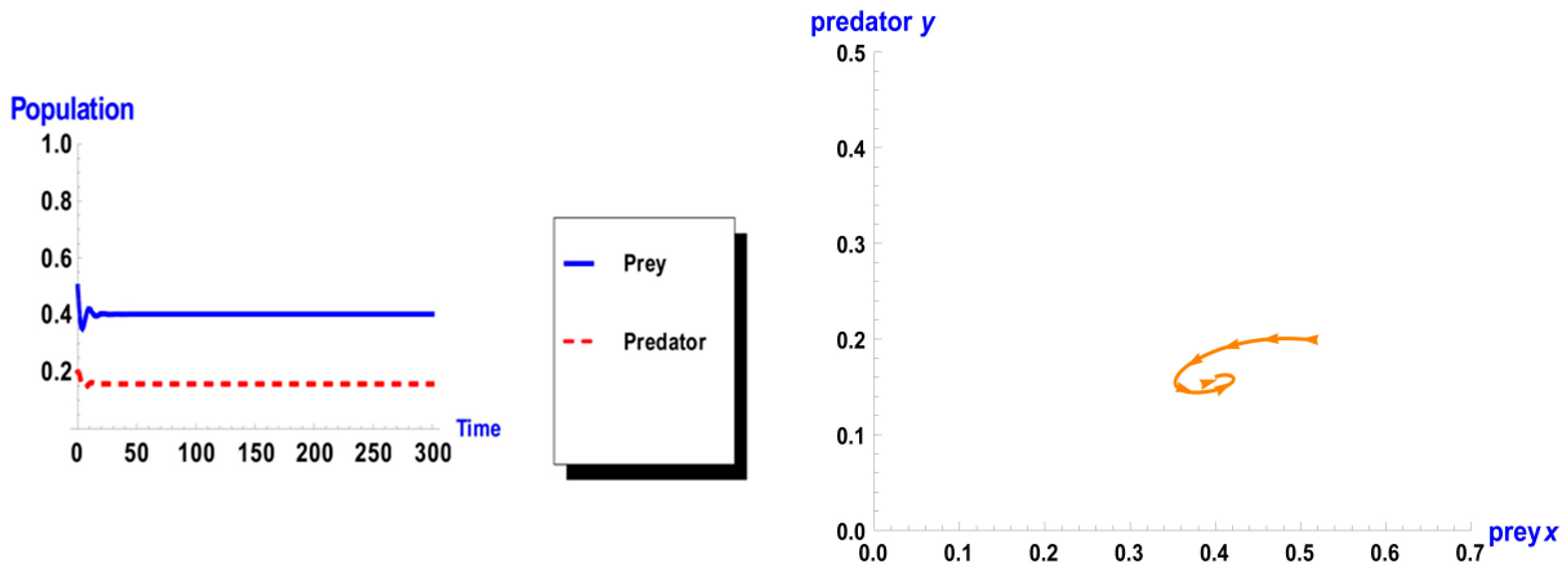
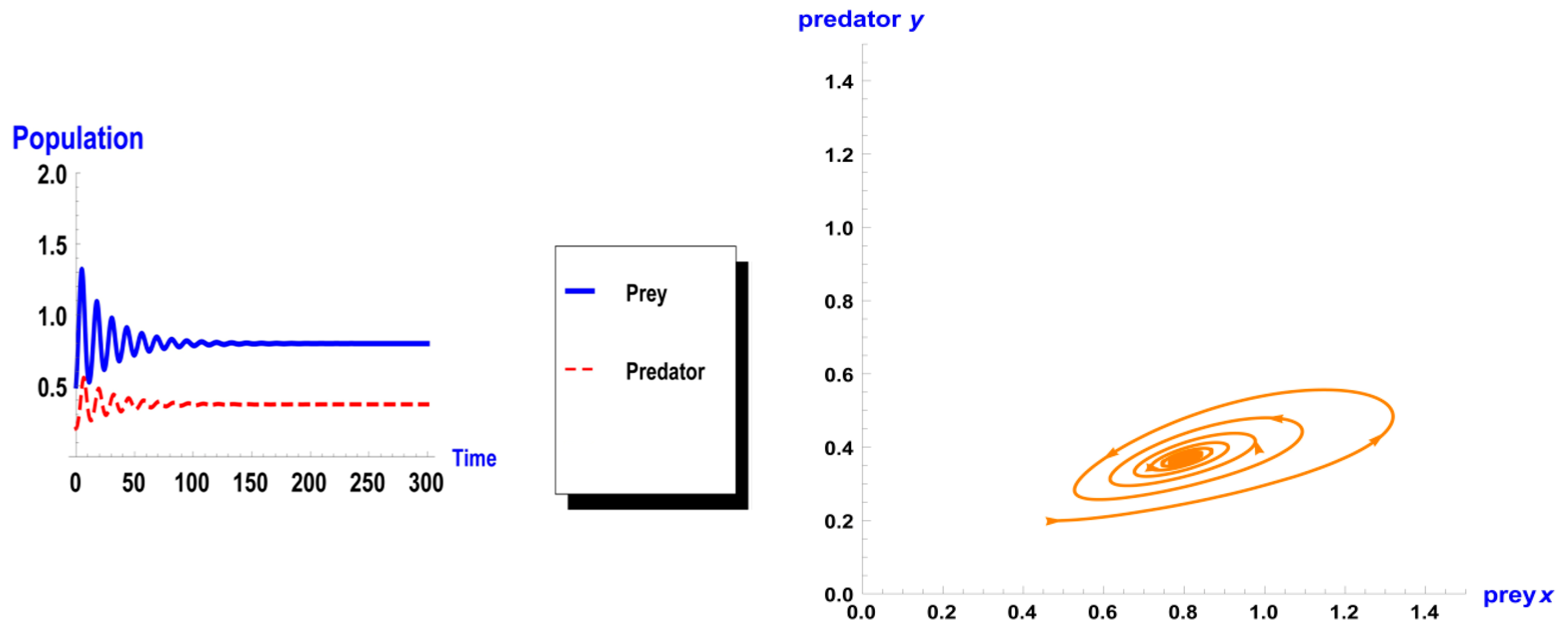
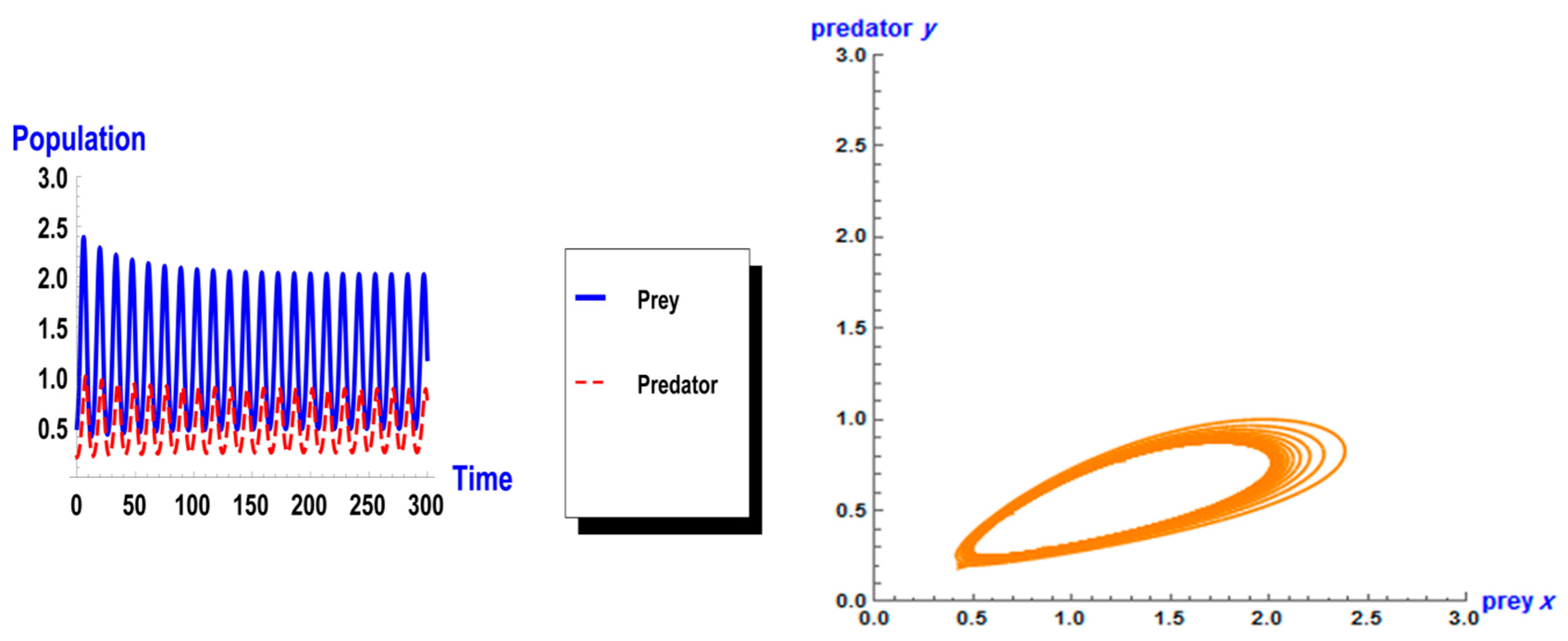
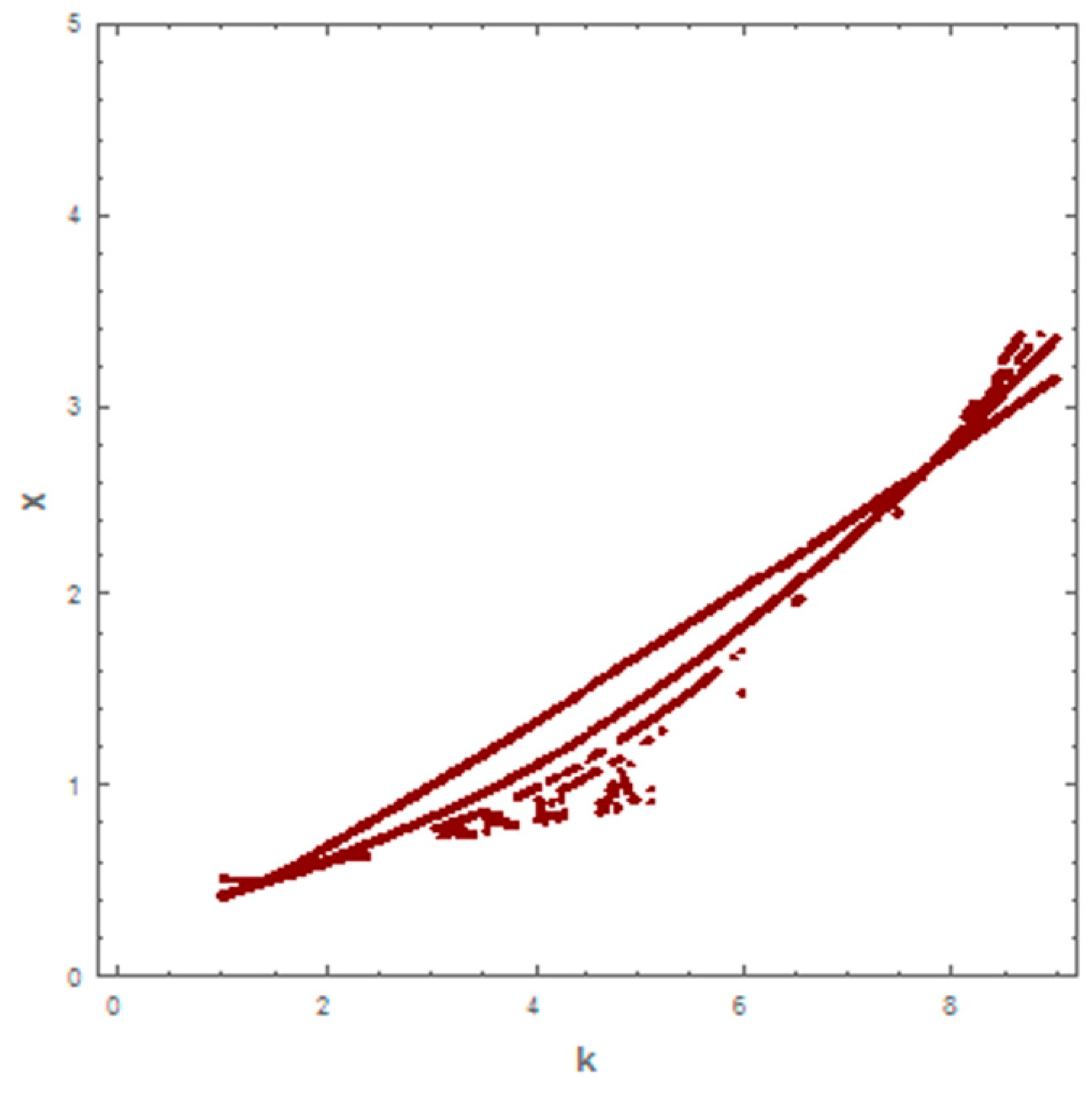
When taking the value of k = 1 of system (1), the dynamic behavior in the first case is stable, as shown in Figure 1. However, when increasing the carrying capacity to k = 4 in the second case, the dynamic behavior oscillates for a period of time and then ends, finally stabilizing, as shown in Figure 2. In the third case, when k = 7, the dynamic behavior oscillates to become a limit cycle, as shown in Figure 3. Consequently, the probability of extinction in the third case would be higher than in the first and second cases. Figure 4 shows the changes of the dynamic behavior of system (1) with Holling type II, from stable to periodic cases. The points in Figure 4 appear because oscillation exists in the dynamic behavior.

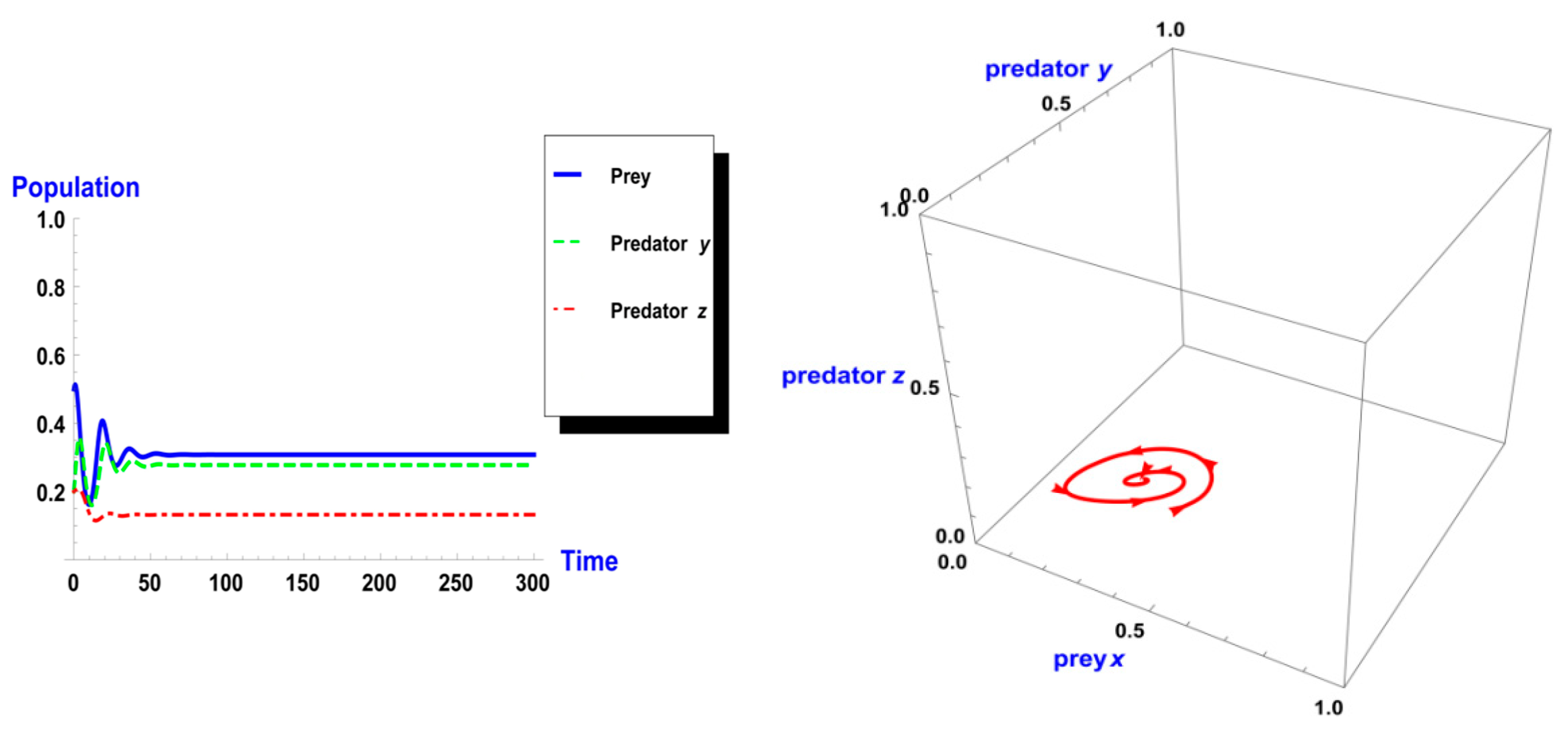
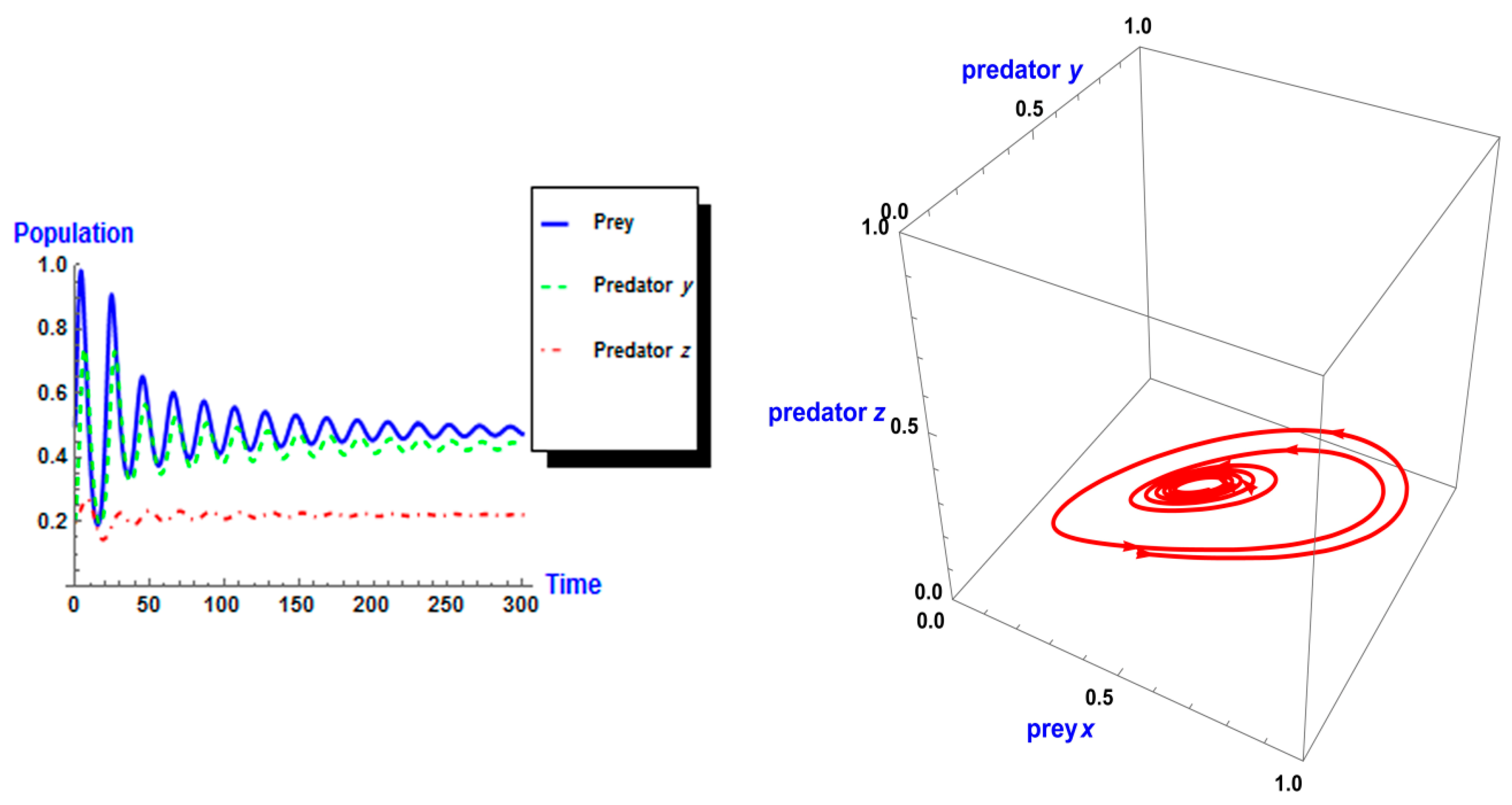
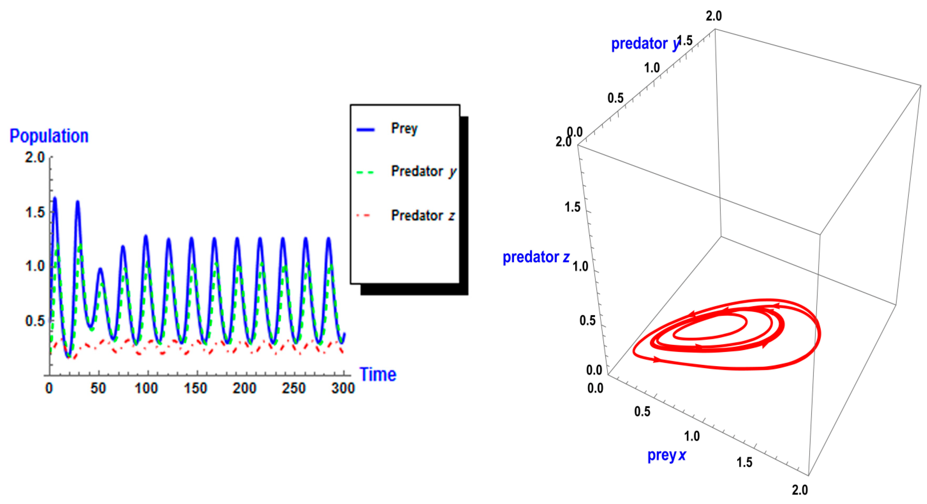
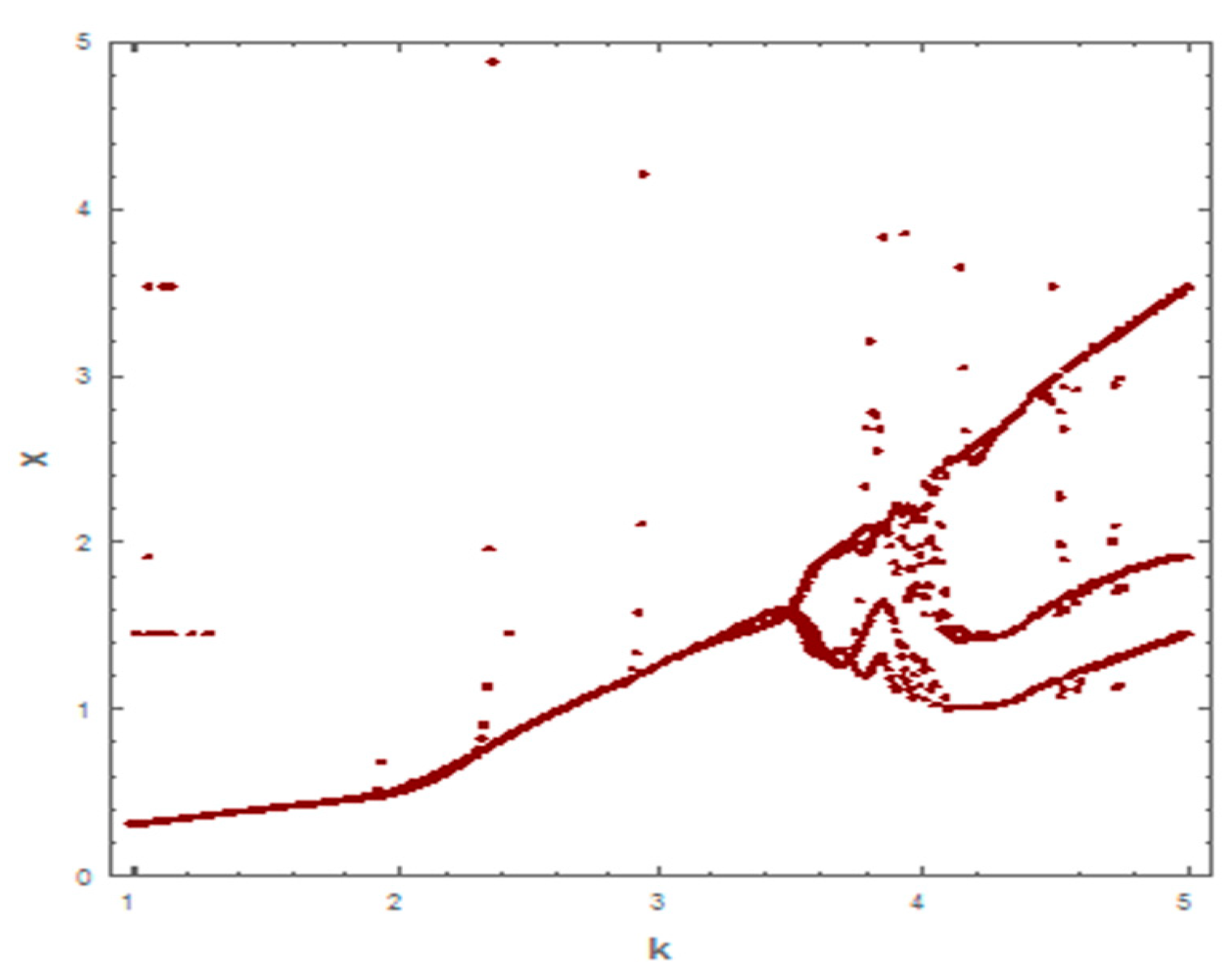
Following the same process, we used different values of k from system (2). As shown in Figure 5, the dynamic behavior is stable when k =1 in the first case. However, when the carrying capacity is increased to k = 2 in the second case, the dynamic behavior oscillates for a period of time and then ends, finally stabilizing, as shown in Figure 6. Whereas in the third case, when k = 3, the dynamic behavior oscillates to create a limit cycle, as shown in Figure 7. Therefore, the probability of extinction in the third case would be greater than in the first and second cases. Figure 8 shows the changes in the dynamic behavior of system (2) with Holling type II, from stable to periodic, quasi-periodic, or chaos cases. The points in Figure 8 appear because oscillation occurs in the dynamic behavior. The numerical simulations show the occurrence of the paradox of enrichment in systems (1) and (2) with Holling type II.

6. Conclusions

We studied the occurrence of the paradox of enrichment in prey–predator models with Holling types I and II functional and numerical responses. We proved through Theorems 1 and 2 that the paradox of enrichment does not occur with Holling type I in two or three dimensions. However, the paradox of enrichment occurs with Holling type II in two and three dimensions, respectively, as shown through Corollary 1, Theorem 5, and the numerical simulations. The numerical simulations explain the occurrence of the paradox of enrichment in systems (1) and (2) with Holling type II when the carrying capacity of prey increases and a map of changes of the dynamic behaviors is given for stable to periodic, quasi-periodic, or chaos cases. We conclude that the linearity and nonlinearity of functional and numerical responses plays important roles in the occurrence of the enrichment paradox. We introduce a new approach connecting the enrichment paradox phenomenon and persistence and extinction dynamics by deriving the persistence and extinction conditions based on the carrying capacity parameter (k). We used different analytical techniques to derive the persistence and extinction conditions. We introduce several theorems and corollaries to present our results. We introduce some biological explanations to support our results.

References

- Liu, H.; Cheng, H. Dynamic analysis of a prey–predator model with state-dependent control strategy and square root response function. Adv. Differ. Equ. 2018, 2018, 63. [Google Scholar] [CrossRef] [Green Version]
- Gurubilli, K.K.; Srinivasu, P.D.N.; Banerjee, M. Global dynamics of a prey-predator model with Allee effect and additional food for the predators. Int. J. Dyn. Control 2017, 5, 903–916. [Google Scholar] [CrossRef]
- Keong, A.T.; Safuan, H.M.; Jacob, K. Dynamical behaviours of prey-predator fishery model with harvesting affected by toxic substances. Matematika 2018, 34, 143–151. [Google Scholar] [CrossRef]
- Heurich, M.; Zeis, K.; Küchenhoff, H.; Müller, J.; Belotti, E.; Bufka, L.; Woelfing, B. Selective predation of a stalking predator on ungulate prey. PLoS ONE 2016, 11, e0158449. [Google Scholar] [CrossRef] [PubMed]
- Gervasi, V.; Nilsen, E.B.; Sand, H.; Panzacchi, M.; Rauset, G.R.; Pedersen, H.C.; Kindberg, J.; Wabakken, P.; Zimmermann, B.; Odden, J.; et al. Predicting the potential demographic impact of predators on their prey: A comparative analysis of two carnivore–ungulate systems in Scandinavia. J. Anim. Ecol. 2012, 81, 443–454. [Google Scholar] [CrossRef] [PubMed]
- Mougi, A.; Iwasa, Y. Evolution towards oscillation or stability in a predator-prey system. Proc. Biol. Sci. 2010, 277, 3163–3171. [Google Scholar] [CrossRef] [PubMed]
- Nowak, E.M.; Theimer, T.C.; Schuett, G.W. Functional and numerical responses of predators: Where do vipers fit in the traditional paradigms? Biol. Rev. Camb. Philos. Soc. 2008, 83, 601–620. [Google Scholar] [CrossRef] [PubMed]
- Griffen, B.D.; Drake, J.M. Effects of habitat quality and size on extinction in experimental populations. Proc. R. Soc. B Biol. Sci. 2008, 275, 2251–2256. [Google Scholar] [CrossRef] [Green Version]
- Haberman, R. Mathematical Models Mechanical Vibrations, Population Dynamics, and Traffic Flow; Society for Industrial and Applied Mathematics: Philadelphia, PA, USA, 1998. [Google Scholar]
- Murray, J.D. Mathematical Biology; Springer: New York, NY, USA, 2002; Volume 2. [Google Scholar]
- Jensen, C.X.J.; Ginzburg, L.R. Paradoxes or theoretical failures? The jury is still out. Ecol. Model. 2005, 188, 3–14. [Google Scholar] [CrossRef]
- Rosenzweig, M.L. Paradox of enrichment—Destabilization of exploitation ecosystems in ecological time. Science 1971, 171, 385–387. [Google Scholar] [CrossRef] [PubMed]
- Walters, C.J.; Krause, E.; Neill, W.E.; Northcote, T.G. Equilibrium-models for seasonal dynamics of plankton biomass in 4 oligotrophic lakes. Can. J. Fish. Aquat. Sci. 1987, 44, 1002–1017. [Google Scholar] [CrossRef]
- McCauley, E.; Murdoch, W.W. Predator prey dynamics in environments rich and poor in nutrients. Nature 1990, 343, 455–457. [Google Scholar] [CrossRef]
- Persson, L.; Johansson, L.; Andersson, G.; Diehl, S.; Hamrin, S.F. Density dependent interactions in lake ecosystems—Whole lake perturbation experiments. Oikos 1993, 66, 193–208. [Google Scholar] [CrossRef]
- Mazumder, A. Patterns of algal biomass in dominant odd-link vs. even-link lake ecosystems. Ecology 1994, 75, 1141–1149. [Google Scholar] [CrossRef]
- Fussmann, G.F.; Ellner, S.P.; Shertzer, K.W.; Hairston, N.G., Jr. Crossing the hopf bifurcation in a live predator–prey system. Science 2000, 290, 1358–1360. [Google Scholar] [CrossRef] [PubMed]
- Cottingham, K.L.; Rusak, J.A.; Leavitt, P.R. Increased ecosystem variability and reduced predictability following fertilisation: Evidence from palaeolimnology. Ecol. Lett. 2000, 3, 340–348. [Google Scholar] [CrossRef]
- Meyer, K.M.; Vos, M.; Mooij, W.M.; Hol, W.H.G.; Termorshuizen, A.J.; van der Putten, W.H. Testing the Paradox of Enrichment along a Land Use Gradient in a Multitrophic Aboveground and Belowground Community. PLoS ONE 2012, 7, e49034. [Google Scholar] [CrossRef] [PubMed] [Green Version]
- Oksanen, L.; Fretwell, S.D.; Arruda, J.; Niemela, P. Exploitation ecosystems in gradients of primary productivity. Am. Nat. 1981, 118, 240–261. [Google Scholar] [CrossRef]
- Freedman, I. Deterministic Mathematical Models in Population Ecology; Marcel Dekker, Inc.: New York, NY, USA, 1980. [Google Scholar]
- Smith, H.L. Competitive coexistence in an oscillating chemostat. SIAM J. Appl. Math. 1981, 40, 498–522. [Google Scholar] [CrossRef]
- Hutson, V.; Vickers, G.A. Criterion for permanent coexistence of species, with an application to a two-prey one-predator system. Math. Biosci. 1983, 63, 253–269. [Google Scholar] [CrossRef]
- Freedman, H.; Waltman, P. Persistence in models of three interacting predator-prey populations. Math. Biosci. 1984, 68, 213–231. [Google Scholar] [CrossRef]
- Waltman, P. Coexistence in chemostat-like models. Rocky Mt. J. Math. 1990, 20, 777–807. [Google Scholar] [CrossRef]
- Ruan, S.; Freedman, H.I. Persistence in three-species food chain models with group defence. Math. Biosci. 1991, 107, 111–125. [Google Scholar] [CrossRef]
- Kuang, Y.; Beretta, E. Global qualitative analysis of a ratio-dependent predator-prey system. J. Math. Biol. 1998, 36, 389–406. [Google Scholar] [CrossRef]
- Kuang, Y. Basic properties of mathematical population models. J. Biomath. 2002, 17, 129–142. [Google Scholar]
- Hsu, S.-B.; Hwang, T.-W.; Kuang, Y. A ratio-dependent food chain model and its applications to biological control. Math. Biosci. 2003, 181, 55–83. [Google Scholar] [CrossRef] [Green Version]
- Dubey, B.; Upadhyay, R. Persistence and extinction of one-prey and two-predator system. Nonlinear Anal. 2004, 9, 307–329. [Google Scholar]
- Gakkhar, S.; Singh, B.; Naji, R.K. Dynamical behavior of two predators competing over a single prey. Biosystems 2007, 90, 808–817. [Google Scholar] [CrossRef] [PubMed]
- Naji, R.K.; Balasim, A.T. Dynamical behavior of a three species food chain model with beddington-deangelis functional response. Chaos Solitons Fractals 2007, 32, 1853–1866. [Google Scholar] [CrossRef]
- Upadhyay, R.K.; Naji, R.K. Dynamics of a three species food chain model with crowley-martin type functional response. Chaos Solitons Fractals 2009, 42, 1337–1346. [Google Scholar] [CrossRef]
- Huo, H.F.; Ma, Z.P.; Liu, C.Y. Persistence and stability for a generalized leslie-gower model with stage structure and dispersal. Abstr. Appl. Anal. 2009, 2009, 135843. [Google Scholar] [CrossRef]
- Kar, T.; Batabyal, A. Persistence and stability of a two prey one predator system. Int. J. Eng. Sci. Technol. 2010, 2, 174–190. [Google Scholar] [CrossRef]
- Tian, X.; Xu, R. Global dynamics of a predator-prey system with holling type II functional response. Nonlinear Anal. Model. Control 2011, 16, 242–253. [Google Scholar]
- Smith, H.L.; Thieme, H.R. Dynamical Systems and Population Persistence; Graduate Studies in Mathematics; AMS: Providence, RI, USA, 2011; Volume 118. [Google Scholar]
- Alebraheem, J.; Abu-Hassan, Y. The Effects of Capture Efficiency on the Coexistence of a Predator in a Two Predators-One Prey Model. J. Appl. Sci. 2011, 11, 3717–3724. [Google Scholar] [CrossRef]
- Alebraheem, J.; Abu-Hassan, Y. Persistence of Predators in a Two Predators-One Prey Model with Non-Periodic Solution. J. Appl. Sci. 2012, 6, 943–956. [Google Scholar]
- Alebraheem, J.; Abu-Hassan, Y. Efficient Biomass Conversion and its Effect on the Existence of Predators in a Predator-Prey System. Res. J. Appl. Sci. 2013, 8, 286–295. [Google Scholar]
- Alebraheem, J.; Abu-Hassan, Y. Dynamics of a two predator–one prey system. Comput. Appl. Math. 2014, 33, 767–780. [Google Scholar] [CrossRef]
- Alebraheem, J. Fluctuations in interactions of prey predator systems. Sci. Int. 2016, 28, 2357–2362. [Google Scholar]
- Hsu, S.B. On global stability of a predator-prey system. Math. Biosci. 1978, 39, 1–10. [Google Scholar] [CrossRef] [Green Version]
- Ameixa, O.M.C.C.; Messelink, G.J.; Kindlmann, P. Nonlinearities Lead to Qualitative Differences in Population Dynamics of Predator-Prey Systems. PLoS ONE 2013, 8, e62530. [Google Scholar] [CrossRef] [PubMed]
- Abu-Hasan, Y.; Alebraheem, J. Functional and Numerical Response in Prey-Predator System. AIP Conf. Proc. 2015, 1651, 3. [Google Scholar] [CrossRef]
- Alebraheem, J.; Abu-Hassan, Y. Simulation of complex dynamical behaviour in prey predator model. In Proceedings of the 2012 International Conference on Statistics in Science, Business and Engineering, Langkawi, Malaysia, 10–12 September 2012. [Google Scholar]
- Smout, S.; Asseburg, C.; Matthiopoulos, J.; Fernández, C.; Redpath, S.; Thirgood, S.; Harwood, J. The Functional Response of a Generalist Predator. PLoS ONE 2010, 5, e10761. [Google Scholar] [CrossRef] [PubMed] [Green Version]
Figure 1.
Dynamic behavior of system (1) when : (a) time series of two trophics x and y; (b) phase space of two trophics.
Figure 2.
Figure 3.
Figure 4.
Bifurcation diagram for system (1) with Holling type II, using carrying capacity (k) as the bifurcation parameter.
Figure 5.
Dynamic behavior of system (2) when : (a) time series of three trophics x, y and z; (b) phase space of three trophics.
Figure 6.
Figure 7.
Figure 8.
Bifurcation diagram for system (2) with Holling type II, using carrying capacity (k) as the bifurcation parameter.
© 2018 by the author. Licensee MDPI, Basel, Switzerland. This article is an open access article distributed under the terms and conditions of the Creative Commons Attribution (CC BY) license (http://creativecommons.org/licenses/by/4.0/).
Share and Cite
MDPI and ACS Style
Alebraheem, J. Relationship between the Paradox of Enrichment and the Dynamics of Persistence and Extinction in Prey-Predator Systems. Symmetry 2018, 10, 532. https://0-doi-org.brum.beds.ac.uk/10.3390/sym10100532
AMA Style
Alebraheem J. Relationship between the Paradox of Enrichment and the Dynamics of Persistence and Extinction in Prey-Predator Systems. Symmetry. 2018; 10(10):532. https://0-doi-org.brum.beds.ac.uk/10.3390/sym10100532
Chicago/Turabian StyleAlebraheem, Jawdat. 2018. "Relationship between the Paradox of Enrichment and the Dynamics of Persistence and Extinction in Prey-Predator Systems" Symmetry 10, no. 10: 532. https://0-doi-org.brum.beds.ac.uk/10.3390/sym10100532
Note that from the first issue of 2016, this journal uses article numbers instead of page numbers. See further details here.