Best Proximity Point Results for Generalized Θ-Contractions and Application to Matrix Equations

Abstract

In this paper, we introduce the notion of $\acute{C}$iri$\acute{c}$ type $\alpha$-$\psi$-$\mathsf{\Theta }$-contraction and prove best proximity point results in the context of complete metric spaces. Moreover, we prove some best proximity point results in partially ordered complete metric spaces through our main results. As a consequence, we obtain some fixed point results for such contraction in complete metric and partially ordered complete metric spaces. Examples are given to illustrate the results obtained. Moreover, we present the existence of a positive definite solution of nonlinear matrix equation $X=Q+{\displaystyle \sum _{i=1}^m}{A}_i^{\ast }\gamma \left(X\right)A_i$ and give a numerical example.

1. Introduction and Preliminaries

In 1922, Polish mathematician Banach [1] proved an interesting result known as “Banach contraction principle" which led to the foundation of metric fixed point theory. His contribution gave a positive answer to the existence and uniqueness of the solution of problems concerned. Later on, many authors extended and generalized Banach’s result in many directions (see [2,3,4]). Samet et al. [5] introduced the contractive condition called $\alpha$-$\psi$-contraction by

$$\alpha (x,y)d(Fx,Fy)\le \psi \left(d\right(x,y\left)\right),$$

where the functions $\psi$: $[0,\infty )\to [0,\infty )$ satisfy the following conditions:

(ψ₁)

$\psi$ is nondecreasing;

(ψ₂)

${\displaystyle \sum _{n=1}^{+\infty }}{\psi }^n\left(t\right)<\infty$ for all $t>0$, where ${\psi }^n$ is the nth iterate of $\psi$ and $\psi \left(t\right)<t$ for any $t>0$;

and that F is $\alpha$-admissible if for all $x,y\in X$

$$\alpha (x,y)\ge 1\Rightarrow \alpha (Fx,Fy)\ge 1,$$

(1)

where $\alpha$: $X\times X\to [0,\infty )$ and proved some fixed point results for such mappings in the context of complete metric spaces $(X,d)$. Subsequently, Salimi et al. [6] and Hussain et al. [2,7] modified the notions of $\alpha$-$\psi$-contractive, $\alpha$-admissible mappings and proved certain fixed point results. In 2014, Jleli et al. [4] generalized the contractive condition by considering a function $\mathsf{\Theta }$: $(0,\infty )\to (1,\infty )$ satisfying,

(Θ₁)

$\mathsf{\Theta }$ is nondecreasing;

(Θ₂)

for each sequence $\left\{{\alpha }_n\right\}\subseteq R^{+},{\lim }_{n\to \infty }\mathsf{\Theta }\left({\alpha }_n\right)=1$ if and only if ${\lim }_{n\to \infty }\left({\alpha }_n\right)=0$;

(Θ₃)

there exist $0<k<1$ and $l\in (0,\infty )$ such that ${\lim }_{\alpha \to 0^{+}}\frac{\mathsf{\Theta }\left(\alpha \right)-1}{{\alpha }^k}=l$,

in the following way,

$$\mathsf{\Theta }\left(d(Fx,Fy)\right)\le {\left[\mathsf{\Theta }\left(d(x,y)\right)\right]}^k,$$

(2)

where $k\in (0,1)$ and $x,y\in X$ and proved the following fixed point theorem.

Theorem 1.

Suppose that F: $X\to X$ is a Θ-contraction, where $(X,d)$ a complete metric space; hen, F possesses a unique $u\in X$ such that $Fu=u$.

Recently, Ahmad et al. [8] used the following weaker condition instead of the condition $\left({\mathsf{\Theta }}_3\right)$:

• (${\mathsf{\Theta }}_3^{\prime }$) $\mathsf{\Theta }$ is continuous on $(0,\infty )$.

Many authors generalized (2) in many directions and proved fixed point theorems for single and multivalued contractive mappings (see [8,9,10]).

However, the mapping involved in all these results were self mappings. For non-empty subsets A and B of a complete metric space $(X,d)$, the contractive mapping $F:A\to B$ may not have a fixed point. The case lead to the search for an element x (say) such that $d(x,Fx)$ is minimum, that is, the distance between the points x and $Fx$ is proximity closed. In view of the fact that $d(x,Fx)\ge d(A,B)$, an absolute optimal approximate solution is an element x for which the error $d(x,Fx)$ assumes the least possible value $d(A,B)$. Thus, a best proximity pair theorem furnishes sufficient conditions for the existence of an optimal approximate solution x, known as a best proximity point of the mapping F, satisfying the condition that $d(x,Fx)=d(A,B)$. Many authors established the existence and convergence of fixed and best proximity points under certain contractive conditions in different metric spaces (see e.g., [11,12,13,14,15,16,17,18,19,20,21,22,23,24,25,26,27,28,29,30] and references therein).

The purpose of this paper is to define the notion of $\acute{C}$iri$\acute{c}$ type $\alpha$-$\psi$-$\mathsf{\Theta }$-contraction and prove some best proximity point results in the frame work of complete metric spaces. Moreover, we prove best proximity point results in partially ordered complete metric spaces through our main results. As an application, we obtain some fixed point results for such contraction in metric and partially ordered metric spaces. Some examples to prove the validity and the existence of solution of nonlinear matrix equation with a numerical example to show the usability of our results is presented.

In the sequel, we denote $\mathsf{\Psi }$ the set of all functions $\psi$ satisfying (${\psi }_1,{\psi }_2$) and $\mathsf{\Omega }$ the set of all functions $\mathsf{\Theta }$ satisfying (${\mathsf{\Theta }}_1,{\mathsf{\Theta }}_2,{\mathsf{\Theta }}_3^{\prime }$).

Let $(X,d)$ be a metric space, A and B two nonempty subsets of $X.$ Define

$$\begin{array}{ccc}\hfill d(A,B)& =& \inf \left\{d\right(a,b):a\in A,b\in B\},\hfill \\ \hfill A_0& =& \{a\in A:\mathrm{there}\mathrm{exists}\mathrm{some}b\in B\mathrm{such}\mathrm{that}d(a,b)=d(A,B\left)\right\},\hfill \\ \hfill B_0& =& \{b\in B:\mathrm{there}\mathrm{exists}\mathrm{some}a\in A\mathrm{such}\mathrm{that}d(a,b)=d(A,B\left)\right\}.\hfill \end{array}$$

Definition 1.

Let $(X,d)$ be a metric space and $A_0\ne \varphi$, we say that the pair $(A,B)$ has the weak P-property if

$$\left\{\begin{array}{c}d(x_1,y_1)=d(A,B)\hfill \\ d(x_2,y_2)=d(A,B)\hfill \end{array}\right.\Rightarrow d(x_1,x_2)\le d(y_1,y_2)$$

for all $x_1,x_2\in A$ and $y_1,y_2\in B.$ [31]

Definition 2.

Let $(X,d)$ be a metric space and $A,B$ two subsets of X, a non-self mapping $T:A\to B$ is called α-proximal admissible if

$$\left\{\begin{array}{c}\alpha (x_1,x_2)\ge 1,\hfill \\ d(u_1,T{x}_1)=d(A,B),\Rightarrow \alpha (u_1,u_2)\ge 1,\hfill \\ d(u_2,T{x}_2)=d(A,B)\hfill \end{array}\right.$$

for all $x_1,x_2,u_1,u_2\in A$, where $\alpha :A\times A\to [0,\infty )$ [4].

2. Best Proximity Point Results for $\stackrel{\mathbf{´}}{\mathit{C}}$iri$\stackrel{\mathbf{´}}{\mathit{c}}$ Type Contraction

We begin this section with the following definition:

Definition 3.

Let $A,B$ be two subsets of a metric space $(X,d)$ and and α: $A\times A\to [0,\infty )$ be a function. A mapping F: $A\to B$ is said to be $\acute{C}$iri$\acute{c}$ type $\alpha$-$\psi$-$\mathsf{\Theta }$-contraction if for $\psi \in \mathsf{\Psi }$, $\mathsf{\Theta }\in \mathsf{\Omega }$, there exists $k\in (0,1)$ and for $x,y\in A$ with $\alpha (x,y)\ge 1$ and $d(Fx,Fy)>0$, we have

$$\alpha (x,y)\mathsf{\Theta }\left[d(Fx,Fy)\right]\le {\left[\psi \left(\mathsf{\Theta }\left(M(x,y)\right)\right)\right]}^k,$$

(3)

where

$$M(x,y)=max\left\{d(x,y),\frac{d(x,Fx)+d(y,Fy)}{2}-d(A,B),\frac{d(x,Fy)+d(y,Fx)}{2}-d(A,B)\right\}.$$

Theorem 2.

Let A and B be two closed subsets of a complete metric space $(X,d)$ with $A_0\ne \varphi$ and let F: $A\to B$ be a $\acute{C}$iri$\acute{c}$ type $\alpha$-$\psi$-$\mathsf{\Theta }$-contraction satisfying

(i) 

F is α-proximal admissible;

(ii) 

$F\left(A_0\right)\subseteq B_0$ and the pair $(A,B)$ satisfies the weak P-property;

(iii) 

F is continuous;

(iv) 

there exist $x_0,x_1\in A_0$ with $d(x_1,F{x}_0)=d(A,B)$ such that $\alpha (x_0,x_1)\ge 1$.

Then, there exists $u\in A$ such that $d(u,Fu)=d(A,B)$.

Proof. 

Consider $x_0$ in $A_0$, since $F\left(A_0\right)\subseteq B_0$, there exists an element $x_1$ in $A_0$ such that $d(x_1,F{x}_0)=d(A,B),$ by assumption (iv), $\alpha (x_0,x_1)\ge 1$. Since $x_1\in A_0$ and $F\left(A_0\right)\subseteq B_0$, there exists $x_2\in A_0$ such that $d(x_2,F{x}_1)=d(A,B).$ By α-proximal admissibility of F, we have that $\alpha (x_1,x_2)\ge 1$. Continuing in this way, we get

$$d(x_{n+1},F{x}_n)=d(A,B)\mathrm{and}\alpha (x_n,x_{n+1})\ge 1\forall n\in \mathbb{N}.$$

(4)

Now if there exists $n_0\in \mathbb{N}$ such that $x_{n_0}=x_{n_0+1}$, we have

$$d(x_{n_0},F{x}_{n_0})=d(x_{n_0+1},F{x}_{n_0})=d(A,B).$$

Then, $x_{n_0}$ is the point of best proximity. Therefore, we assume that $x_n\ne x_{n+1}$, i.e., $d(x_n,x_{n+1})>0$ for all $n\in \mathbb{N}\cup \left\{0\right\}$.

By weak P-property of the pair $(A,B)$ and from (3), (4), we have for all $n\in \mathbb{N}$

$$\begin{array}{ccc}\hfill 1<\mathsf{\Theta }\left[d(x_{n+1},x_n)\right]& \le & \mathsf{\Theta }\left[d(F{x}_n,F{x}_{n-1})\right]\hfill \\ & \le & \alpha (x_n,x_{n-1})\mathsf{\Theta }\left[d(F{x}_n,F{x}_{n-1})\right]\hfill \\ & \le & {\left[\psi \left(\mathsf{\Theta }\left(M(x_n,x_{n-1})\right)\right)\right]}^k,\hfill \end{array}$$

(5)

where

$$\begin{array}{ccc}M(x_n,x_{n-1})\hfill & =\hfill & max\left\{d(x_n,x_{n-1}),\frac{d(x_n,F{x}_n)+d(x_{n-1},F{x}_{n-1})}{2}-d(A,B),\right.\hfill \\ & & \left.\frac{d(x_n,F{x}_{n-1})+d(x_{n-1},F{x}_n)}{2}-d(A,B)\right\}\hfill \\ & \le \hfill & max\left\{d(x_n,x_{n-1}),\frac{d(x_n,x_{n+1})+d(x_{n+1},F{x}_n)+d(x_{n-1},x_n)+d(x_n,F{x}_{n-1})}{2}-d(A,B),\right.\hfill \\ & & \left.\frac{d(x_n,F{x}_{n-1})+d(x_{n-1},x_{n+1})+d(x_{n+1},F{x}_n)}{2}-d(A,B)\right\}\hfill \\ & =\hfill & max\left\{d(x_n,x_{n-1}),\frac{d(x_n,x_{n+1})+d(x_{n-1},x_n)}{2},\frac{d(x_{n-1},x_{n+1})}{2}\right\}\hfill \\ & \le \hfill & max\left\{d(x_n,x_{n-1}),\frac{d(x_n,x_{n+1})+d(x_{n-1},x_n)}{2}\right\}\hfill \\ & \le \hfill & max\left\{d(x_n,x_{n-1}),d(x_n,x_{n+1})\right\}.\hfill \end{array}$$

This together with inequality (5) gives

$$1<\mathsf{\Theta }\left[d(x_n,x_{n+1})\right]\le {\left[\psi \left(\mathsf{\Theta }\left(max\{d(x_n,x_{n-1}),d(x_n,x_{n+1})\}\right)\right)\right]}^k.$$

If

$$max\{d(x_n,x_{n-1}),d(x_n,x_{n+1})\}=d(x_n,x_{n+1}),$$

we have

$$\begin{array}{ccc}\hfill 1<\mathsf{\Theta }\left[d(x_n,x_{n+1})\right]& \le & {\left[\psi \left(\mathsf{\Theta }\left(d(x_n,x_{n+1})\right)\right)\right]}^k\hfill \\ & <& \mathsf{\Theta }\left(d(x_n,x_{n+1})\right),\hfill \end{array}$$

a contradiction, so we have

$$1<\mathsf{\Theta }\left[d(x_n,x_{n+1})\right]\le {\left[\psi \left(\mathsf{\Theta }\left(d(x_n,x_{n-1})\right)\right)\right]}^k.$$

By induction, we get

$$\begin{array}{ccc}\hfill 1<\mathsf{\Theta }\left[d(x_n,x_{n+1})\right]& \le & {\left[\psi \left(\mathsf{\Theta }\left(d(x_{n-1},x_n)\right)\right)\right]}^k\hfill \\ & \le & {\left[\psi \left(\mathsf{\Theta }\left(d(x_{n-2},x_{n-1})\right)\right)\right]}^{k^2}\hfill \\ & & .\hfill \\ & & .\hfill \\ & & .\hfill \\ & \le & {\left[\psi \left(\mathsf{\Theta }\left(d(x_0,x_1)\right)\right)\right]}^{k^n}.\hfill \end{array}$$

Taking limit as $n\to \infty$ in above inequality, we have

$$\mathsf{\Theta }\left[d(x_n,x_{n+1})\right]\to 1$$

and by ${\mathsf{\Theta }}_2$, we obtain

$$\underset{n\to \infty }{\lim }d(x_n,x_{n+1})=0.$$

(6)

Now, we show that $\left\{x_n\right\}$ is a Cauchy sequence in A. Suppose on the contrary that it is not, that is, ∃$ϵ>0$, we can find the sequences $\left\{p_n\right\}$ and $\left\{q_n\right\}$ of natural numbers such that for $p_n>q_n>n$, we have

$$d(x_{p_n},x_{q_n})\ge ϵ.$$

Then,

$$d(x_{p_n-1},x_{q_n})<ϵ$$

(7)

for all $n\in \mathbb{N}$. Thus, by triangle inequality and (7), we get

$$\begin{array}{c}\hfill ϵ\le d(x_{p_n},x_{q_n})\le d(x_{p_n},x_{p_n-1})+d(x_{p_n-1},x_{q_n})<d(x_{p_n},x_{p_n-1})+ϵ.\end{array}$$

Taking limit and using inequality (6), we get

$$\underset{n\to \infty }{\lim }d(x_{p_n},x_{q_n})=ϵ.$$

(8)

Again by triangle inequality, we have

$$\begin{array}{c}\hfill d(x_{p_n},x_{q_n})\le d(x_{p_n},x_{p_n+1})+d(x_{p_n+1},x_{q_n+1})+d(x_{q_n+1},x_{q_n})\end{array}$$

(9)

and

$$\begin{array}{c}\hfill d(x_{p_n+1},x_{q_n+1})\le d(x_{p_n+1},x_{p_n})+d(x_{p_n},x_{q_n})+d(x_{q_n},x_{q_n+1}).\end{array}$$

(10)

Taking limit as $n\to \infty$, from Equations (6) and (8), we have that

$$\underset{n\to \infty }{\lim }d(x_{p_n+1},x_{q_n+1})=ϵ.$$

(11)

Thus, Equation (8) holds. Then by assumption, $\alpha (x_{p_n},x_{q_n})\ge 1$, we get

$$\begin{array}{ccc}\hfill 1\le \mathsf{\Theta }\left(d(x_{p_n+1},x_{q_n+1})\right)& \le & \mathsf{\Theta }\left(d(F{x}_{p_n},F{x}_{q_n})\right)\hfill \\ & \le & \alpha (x_{p_n},x_{q_n})\mathsf{\Theta }\left(d(F{x}_{p_n},F{x}_{q_n})\right)\hfill \\ & \le & {\left[\psi \left(\mathsf{\Theta }\left(M(x_{p_n},x_{q_n})\right)\right)\right]}^k\hfill \\ & <& \mathsf{\Theta }\left(M(x_{p_n},x_{q_n})\right).\hfill \end{array}$$

By taking limit as $n\to \infty$ in above inequality, using (${\mathsf{\Theta }}_3^{{}^{\prime }}$) and Equation (6), we get

$$\underset{n\to \infty }{\lim }d(x_{p_n},x_{q_n})=0<ϵ,$$

which is a contradiction. Thus, $\left\{x_n\right\}$ is a Cauchy sequence. Since $\left\{x_n\right\}\subseteq A$ and A is closed in a complete metric space $(X,d)$, we can find $u\in A$ such that $x_n\to u$. Since F is continuous, we have $F{x}_n\to Fu$. This implies that $d(x_{n+1},F{x}_n)\to d(u,Fu)$.

Since the sequence $\left\{d(x_{n+1},F{x}_n)\right\}$ is a constant sequence with value $d(A,B)$, we deduce

$$d(u,Fu)=d(A,B).$$

This completes the proof. □

Example 1.

Let $X={\mathbb{R}}^2$ with metric d defined as $d((x_1,x_2),(y_1,y_2))=|x_1-y_1|+|x_2-y_2|.$ Suppose $A=\left\{\right(-4,-4),(-7,-8),(20,0),(25,30\left)\right\}$ and $B=\left\{\right(-4,0),(0,-4),(-9,-10),(-11,-8\left)\right\}$. Then, $d(A,B)=4$, $A_0=\{(-4,-4),(-7,-8)\}$ and $B_0=\{(-4,0),(0,-4),(-9,-10),(-11,-8)\}$. Define $F:A\to B$ by $F(-4,-4)=(-9,-10),F(-7,-8)=(-11,-8),F(20,0)=(-4,0),F(25,30)=(0,-4)$ and $\alpha :A\times A\to [0,\infty )$ by $\alpha ((x,y),(u,v))=\frac{11}{10}$. Clearly, $F\left(A_0\right)\subseteq B_0.$ Now, let $(-4,-4),(-7,-8)\in A$ and $(-4,0),(-9,-10)\in B$ such that

$$\left\{\begin{array}{c}d\left(\right(-4,-4),(-4,0\left)\right)=d(A,B)=4,\hfill \\ d\left(\right(-7,-8),(-9,-10\left)\right)=d(A,B)=4.\hfill \end{array}\right.\Rightarrow d((-4,-4),(-7,-8))<d((-4,0),(-9,-10)).$$

Similarly, for all $(x_1,y_1),(x_2,y_2)\in A$ and $(u_1,v_1),(u_2,v_2)\in B$, we have

$$\left\{\begin{array}{c}d((x_1,y_1),(u_1,v_1))=d(A,B)\hfill \\ d((x_2,y_2),(u_2,v_2))=d(A,B)\hfill \end{array}\right.\Rightarrow d((x_1,y_1),(x_2,y_2))<d((u_1,v_1),(u_2,v_2)),$$

that is, the pair $(A,B)$ has weak P-property. Suppose

$$\left\{\begin{array}{c}\alpha \left(\right(-7,-8),(20,0\left)\right)\ge 1,\hfill \\ d\left(\right(-9,-10),(-11,-8\left)\right)=d(A,B)=4,\hfill \\ d\left(\right(-4,-4),(-4,0\left)\right)=d(A,B)=4,\hfill \end{array}\right.$$

then $\alpha ((-9,-10),(-4,-4))=\frac{11}{10}>1$. Hence, $\alpha \left(\right(x,y),(u,v\left)\right)\ge 1$ for all $x,y,u,v\in A$. Thus, F is α-proximal admissible mapping. Now, we show that F is $\acute{C}$iri$\acute{c}$ type $\alpha$-$\psi$-$\mathsf{\Theta }$ contraction. For ((−4, −4), (20, 0)), define ψ: $[0,\infty )\to [0,\infty )$ by $\psi \left(t\right)=\frac{999}{1000}t$ and Θ: $(0,\infty )\to (1,\infty )$ by $\mathsf{\Theta }\left(t\right)=t+1$.

Now,

$$\alpha ((-4,-4),(20,0))\mathsf{\Theta }\left[d(F(-4,-4),F(20,0))\right]=\frac{88}{5}$$

(12)

and for

$$\begin{array}{cc}& M\left(\right(-4,-4),(20,0\left)\right)\hfill \\ =& max\{d((-4,-4),(20,0)),\frac{d\left(\right(-4,-4),F(-4,-4\left)\right)+d\left(\right(20,0),F(20,0\left)\right)}{2}-d(A,B),\hfill \\ & \frac{d\left(\right(-4,-4),F(20,0\left)\right)+d\left(\right(20,0),F(-4,-4\left)\right)}{2}-d(A,B)\}\hfill \\ =& max\{28,\frac{d\left(\right(-4,-4),(-9,-10\left)\right)+d\left(\right(20,0),(-4,0\left)\right)}{2}-4,\hfill \\ & \frac{d\left(\right(-4,-4),(-4,0\left)\right)+d\left(\right(20,0),(-9,-10\left)\right)}{2}-4\}\hfill \\ =& 28,\hfill \end{array}$$

we have

$${\left[\psi \left(\mathsf{\Theta }\left(M((4,1),(7,4))\right)\right)\right]}^k={\left(\frac{999}{1000}\left(29\right)\right)}^k.$$

(13)

Hence, from Equation (12), (13) and for $k=0.83$, we have

$$\frac{88}{5}<{\left(\frac{999}{1000}\left(29\right)\right)}^k.$$

Similarly, inequality holds for the remaining cases. Hence, all the assertions of Theorem 2 are satisfied and F has a best proximity point $(-7,-8)$.

Example 2.

Let $X={\mathbb{R}}^2$ with metric d defined as $d((x_1,x_2),(y_1,y_2))=|x_1-y_1|+|x_2-y_2|.$ Suppose $A=(-\infty ,-1]\times \left\{1\right\}$ and $B=\left\{0\right\}\times [\frac{5}{4},+\infty )$. Then, $d(A,B)=d((-1,1),(0,\frac{5}{4}))=\frac{5}{4}$ and $A_0=\left\{(-1,1)\right\},B_0=\left\{(0,\frac{5}{4})\right\}$. Define $F:A\to B$ by

$$F(x,1)=\left\{\begin{array}{cc}(0,-x+|x+3\left|\right|x+4\left|e^{-x}\right)\hfill & ifx\in (-\infty ,-2),\hfill \\ (0,\frac{-x}{4}+1)\hfill & ifx\in [-2,-1],\hfill \end{array}\right.$$

and $\alpha :A\times A\to [0,\infty )$ by

$$\alpha ((x,y),(u,v))=\left\{\begin{array}{cc}1,\hfill & if(x,y),(u,v)\in [-2,-1]\times [-2,-1],\hfill \\ 0,\hfill & otherwise.\hfill \end{array}\right.$$

Clearly, $F\left(A_0\right)\subseteq B_0.$ Now, let $(x_1,1),(x_2,1)\in A$ and $(0,u_1),(0,u_2)\in B$ such that

$$\left\{\begin{array}{c}d((x_1,1),(0,u_1))=d(A,B)=\frac{5}{4},\hfill \\ d((x_2,1),(0,u_2))=d(A,B)=\frac{5}{4}.\hfill \end{array}\right.$$

Necessarily, $(x_1=u_1\in [-2,-1])$ and $(x_2=u_2\in [-2,-1])$. In this case,

$$d((x_1,1),(x_2,1))=d((0,u_1),(0,u_2)),$$

that is, the pair $(A,B)$ has weak P-property.

Suppose

$$\left\{\begin{array}{c}\alpha ((x_1,1),(x_2,1))\ge 1,\hfill \\ d((u_1,1),F(x_1,1))=d(A,B)=\frac{5}{4},\hfill \\ d((u_2,1),F(x_2,1))=d(A,B)=\frac{5}{4},\hfill \end{array}\right.$$

then

$$\left\{\begin{array}{c}(x_1,1),(x_2,1)\in [-2,-1],\hfill \\ d((u_1,1),F(x_1,1))=\frac{5}{4},\hfill \\ d((u_2,1),F(x_2,1))=\frac{5}{4}.\hfill \end{array}\right.$$

Thus, $(x_1,x_2)\in [-2,-1]\times [-2,-1]$. We also have $u_1=\frac{-x}{4}+1and{u}_2=\frac{-x}{4}+1,$ that is $(u_1=\frac{-x}{4}+1,1)$, $(u_2=\frac{-x}{4}+1,1)\in [-2,-1]\times [-2,-1]$. Thus, $\alpha ((u_1,1),(u_2,1))\ge 1$. That is, F is an α-proximal admissible mapping. Now, we show that F is $\acute{C}$iri$\acute{c}$ type $\alpha$-$\psi$-$\mathsf{\Theta }$ contraction. For this, define ψ: $[0,\infty )\to [0,\infty )$ by $\psi \left(t\right)=\frac{999}{1000}t$ and Θ: $(0,\infty )\to (1,\infty )$ by $\mathsf{\Theta }\left(t\right)=t+1$. We will verify the following inequality

$$\alpha ((x,1),(y,1))\mathsf{\Theta }\left[d(F(x,1),F(y,1))\right]\le {\left[\psi \left(\mathsf{\Theta }(M(x,1),(y,1))\right)\right]}^k,$$

(14)

where $k\in (0,1).$ The left-hand side of inequality (14) gives

$$\alpha ((x,1),(y,1))\mathsf{\Theta }\left[d(F(x,1),F(y,1))\right]=\frac{|x-y|}{4}+1$$

and the right side of inequality (14) is

$${\left[\psi \left(\mathsf{\Theta }\left(M((x,1),(y,1))\right)\right)\right]}^k,$$

where

$$\begin{array}{ccc}\hfill M((x,1),(y,1))& =& max\left\{d((x,1),(y,1)),\frac{d((x,1),F(x,1))+d((y,1),F(y,1))}{2}-d(A,B),\right.\hfill \\ & & \left.\frac{d((x,1),F(y,1))+d((y,1),F(x,1))}{2}-d(A,B)\right\}\hfill \\ & =& max\left\{d((x,1),(y,1)),\frac{d((x,1),(0,\frac{-x}{4}+1))+d((y,1),(0,\frac{-y}{4}+1))}{2}-\frac{5}{4},\right.\hfill \\ & & \left.\frac{d((x,1),(0,\frac{-y}{4}+1))+d((y,1),(0,\frac{-x}{4}+1))}{2}-\frac{5}{4}\right\}\hfill \\ & =& max\left\{|x-y|,\frac{\left|x\right|+|1+\frac{x}{4}-1|+|y|+|1+\frac{y}{4}-1|}{2}-\frac{5}{4},\right.\hfill \\ & & \left.\frac{\left|x\right|+|1+\frac{y}{4}-1|+|y|+|1+\frac{x}{4}-1|}{2}-\frac{5}{4}\right\}\hfill \\ & =& max\left\{|x-y|,\frac{\left|x\right|+|1+\frac{x}{4}-1|+|y|+|1+\frac{y}{4}-1|}{2}-\frac{5}{4}\right\}\hfill \\ & =& max\left\{|x-y|,\frac{\left|x\right|+|\frac{x}{4}|+|y|+|\frac{y}{4}|}{2}-\frac{5}{4}\right\}.\hfill \end{array}$$

If $max\{|x-y|,\frac{\left|x\right|+|\frac{x}{4}|+|y|+|\frac{y}{4}|}{2}-\frac{5}{4}\}=|x-y|$, then inequality (14) becomes

$$\begin{array}{c}\hfill \frac{|x-y|}{4}+1\le \left[\psi \right(\mathsf{\Theta }\left(\right|x-{y\left|\right)\left)\right]}^k={\left[\psi \right(|x-y|+1\left)\right]}^k<\psi \left(\right|x-y|+1)=\frac{999}{1000}\left(\right|x-y|+1).\end{array}$$

Thus, $\frac{|x-y|}{4}+1<\frac{999}{1000}\left(\right|x-y|+1)$, which is true.

Now, if

$$max\left\{|x-y|,\frac{\left|x\right|+|\frac{x}{4}|+|y|+|\frac{y}{4}|}{2}-\frac{5}{4}\right\}=\frac{\left|x\right|+|\frac{x}{4}|+|y|+|\frac{y}{4}|}{2}-\frac{5}{4},$$

then

$$\begin{array}{ccc}\hfill \frac{|x-y|}{4}+1& \le & {\left[\psi (\mathsf{\Theta }(\frac{\left|x\right|+|\frac{x}{4}|+|y|+|\frac{y}{4}|}{2}-\frac{5}{4}))\right]}^k\hfill \\ & =& {\left[\psi (2(\left|x\right|+|\frac{x}{4}|+|y|+|\frac{y}{4}|)-4)\right]}^k\hfill \\ & <& \psi \left(2(|x|+|\frac{x}{4}|+|y|+|\frac{y}{4}|)-4\right)\hfill \\ & =& \frac{999}{1000}\left[2\left(\left|x\right|+|\frac{x}{4}|+|y|+|\frac{y}{4}|-2\right)\right]\hfill \end{array}$$

implies

$$\frac{|x-y|}{4}+1<\frac{999}{1000}[2\left(\left|x\right|+|\frac{x}{4}|+|y|+|\frac{y}{4}|-2\right)],$$

which is also true. Thus, F is $\acute{C}$iri$\acute{c}$ type $\alpha$-$\psi$-$\mathsf{\Theta }$ contraction. Similar argument holds for the rest of the interval. Hence, all the hypotheses of Theorem 2 are verified. Thus F has best proximity point $(-1,1)$.

Condition of continuity of the mapping in Theorem 2 can be replaced with the following condition to prove the existence of best proximity point of F: $\mathcal{H}$: If $\left\{x_n\right\}$ is a sequence in A such that $\alpha (x_n,x_{n+1})\ge 1$ for all n and $x_n\to x\in A$ as $n\to \infty$, then there exists a subsequence $\left\{x_{n\left(p\right)}\right\}$ of {$x_n\}$ such that $\alpha (x_{n\left(p\right)},x)\ge 1$ for all p.

Theorem 3.

Let A and B be two closed subsets of a complete metric space $(X,d)$ with $A_0\ne \varphi$ and let F: $A\to B$ be a $\acute{C}$iri$\acute{c}$ type $\alpha$-$\psi$-$\mathsf{\Theta }$-contraction satisfying

(i) 

F is α-proximal admissible;

(ii) 

$F\left(A_0\right)\subseteq B_0$ and the pair $(A,B)$ satisfies the weak P-property;

(iii) 

there exists $x_0,x_1\in A_0$ with $d(x_1,F{x}_0)=d(A,B)$ such that $\alpha (x_0,x_1)\ge 1$;

(iv) 

condition $\mathcal{H}$ holds.

Then, there exists $u\in A$ such that $d(u,Fu)=d(A,B)$.

Proof. 

Following the proof of Theorem 2, there is a Cauchy sequence $\left\{x_n\right\}$ in A such that $x_n\to u\in A$. Then, by condition (iv), there exists a subsequence $\left\{x_{n\left(p\right)}\right\}$ of {$x_n\}$ such that $\alpha (x_{n\left(p\right)},u)\ge 1$ for all p. Since F is $\acute{C}$iri$\acute{c}$ type $\alpha$-$\psi$-$\mathsf{\Theta }$-contraction, we have by weak P-property and for all p

$$\begin{array}{ccc}1\le \mathsf{\Theta }\left(d(x_{n\left(p\right)+1},u)\right)\le \mathsf{\Theta }\left(d(F{x}_{n\left(p\right)},Fu)\right)\hfill & \le \hfill & \alpha (x_{n\left(p\right)},u)\mathsf{\Theta }\left(d(F{x}_{n\left(p\right)},Fu)\right)\hfill \\ & \le \hfill & {\left[\psi \left(\mathsf{\Theta }\left(M(x_{n\left(p\right)},u)\right)\right)\right]}^k,\hfill \end{array}$$

(15)

where

$$\begin{array}{ccc}M(x_{n\left(p\right)},u)\hfill & =\hfill & max\{d(x_{n\left(p\right)},u),\frac{d(x_{n\left(p\right)},F{x}_{n\left(p\right)})+d(u,Fu)}{2}-d(A,B),\hfill \\ & & \frac{d(x_{n\left(p\right)},Fu)+d(u,F{x}_{n\left(p\right)})}{2}-d(A,B)\}\hfill \\ & \le \hfill & max\{d(x_{n\left(p\right)},u),\frac{d(x_{n\left(p\right)},x_{n\left(p\right)+1})+d(x_{n\left(p\right)+1},F{x}_{n\left(p\right)})+d(u,Fu)}{2}-d(A,B),\hfill \\ & & \frac{d(x_{n\left(p\right)},u)+d(u,Fu)+d(u,x_{n\left(p\right)+1})+d(x_{n\left(p\right)+1},F{x}_{n\left(p\right)})}{2}-d(A,B)\}\hfill \\ & =\hfill & max\{d(x_{n\left(p\right)},u),\frac{d(x_{n\left(p\right)},x_{n\left(p\right)+1})+d(A,B)+d(u,Fu)}{2}-d(A,B),\hfill \\ & & \frac{d(x_{n\left(p\right)},u)+d(u,Fu)+d(u,x_{n\left(p\right)+1})+d(A,B)}{2}-d(A,B)\}.\hfill \end{array}$$

(16)

Letting $p\to \infty$ in the above inequality, we get that

$$\underset{p\to \infty }{\lim }M(x_{n\left(p\right)},u)\le \frac{d(u,Fu)-d(A,B)}{2}.$$

(17)

Furthermore,

$$\begin{array}{ccc}\hfill d(u,Fu)& \le & d(u,x_{n\left(p\right)+1})+d(x_{n\left(p\right)+1},F{x}_{n\left(p\right)})+d(F{x}_{n\left(p\right)},Fu)\hfill \\ & \le & d(u,x_{n\left(p\right)+1})+d(A,B)+d(F{x}_{n\left(p\right)},Fu),\hfill \end{array}$$

which gives

$$d(u,Fu)-d(A,B)-d(u,x_{n\left(p\right)+1})\le d(F{x}_{n\left(p\right)},Fu).$$

(18)

Taking $p\to \infty$ in inequality (18), we get

$$d(u,Fu)-d(A,B)\le \underset{p\to \infty }{\lim }d(F{x}_{n\left(p\right)},Fu).$$

(19)

By (15), we have

$$\begin{array}{c}\hfill \mathsf{\Theta }\left(d(F{x}_{n\left(p\right)},Fu)\right)\le {\left[\psi \left(\mathsf{\Theta }\left(M(x_{n\left(p\right)},u)\right)\right)\right]}^k<\mathsf{\Theta }\left(M(x_{n\left(p\right)},u)\right),\end{array}$$

(20)

which implies

$$\begin{array}{c}\hfill d(F{x}_{n\left(p\right)},Fu)\le M(x_{n\left(p\right)},u).\end{array}$$

(21)

Taking limit as $p\to \infty$ in inequality (21), we obtain

$$d(u,Fu)-d(A,B)\le \frac{d(u,Fu)-d(A,B)}{2},$$

which is a contradiction. Hence, $d(u,Fu)=d(A,B)$. □

For the uniqueness of best proximity point, we use the following condition:

$\mathcal{U}$: For all $x,y\in BPP\left(F\right)$, $\alpha (x,y)\ge 1$, where BPP(F) denote the set of best proximity points of F.

Theorem 4.

Adding condition $\mathcal{U}$ to the hypotheses of Theorem 2 (resp., Theorem 3), one obtains a unique u in A such that $d(u,Fu)=d(A,B)$.

Proof. 

Suppose that u and v are two best proximity points of F with $u\ne v$, that is, $d(u,Fu)=d(A,B)=d(v,Fv)$. Then, by $\mathcal{U},$

$$\alpha (u,v)\ge 1.$$

(22)

Since the pair $(A,B)$ has the weak P-property, from inequality (3), we have

$$\begin{array}{ccc}\mathsf{\Theta }\left(d\right(u,v\left)\right)\le \mathsf{\Theta }\left(d\right(Fu,Fv\left)\right)\hfill & \le \hfill & \alpha (u,v)\mathsf{\Theta }\left(d\right(Fu,Fv\left)\right)\hfill \\ & \le \hfill & {\left[\psi \left(\mathsf{\Theta }\left(M(u,v)\right)\right)\right]}^k\hfill \\ & =\hfill & {\left[\psi \left(\mathsf{\Theta }\left(d(u,v)\right)\right)\right]}^k\hfill \\ & <\hfill & \mathsf{\Theta }\left(d\right(u,v\left)\right),\hfill \end{array}$$

(23)

which is a contradiction, so $u=v$. □

If we take $M(x,y)=d(x,y)$ in Theorem 2, we have the following corollary:

Corollary 1.

Let A and B be two closed subsets of a complete metric space $(X,d)$ with $A_0\ne \varphi$ and let F: $A\to B$ be a mapping satisfying

(i) 

$\alpha (x,y)\mathsf{\Theta }\left[d(Fx,Fy)\right]\le {\left[\psi \left(\mathsf{\Theta }\left(d(x,y)\right)\right)\right]}^k$;

(ii) 

F is continuous α-proximal admissible;

(iii) 

$F\left(A_0\right)\subseteq B_0$ and the pair $(A,B)$ satisfies the weak P-property;

(iv) 

there exist $x_0,x_1\in A_0$ with $d(x_1,F{x}_0)=d(A,B)$ such that $\alpha (x_0,x_1)\ge 1$.

Then, there exists $u\in A$ such that $d(u,Fu)=d(A,B)$.

If $\alpha (x,y)=1$ for all $x,y\in A$ in Theorem 2, we have

Corollary 2.

Let A and B be two closed subsets of a complete metric space $(X,d)$ with $A_0\ne \varphi$ and let F: $A\to B$ be a mapping satisfying

(i) 

$\mathsf{\Theta }\left[d(Fx,Fy)\right]\le {\left[\psi \left(\mathsf{\Theta }\left(M(x,y)\right)\right)\right]}^k$;

(ii) 

$F\left(A_0\right)\subseteq B_0$ and the pair $(A,B)$ satisfies the weak P-property;

(iii) 

F is continuous;

(iv) 

there exist $x_0,x_1\in A_0$ such that $d(x_1,F{x}_0)=d(A,B)$;

Then, there exists $u\in A$ such that $d(u,Fu)=d(A,B)$.

If $M(x,y)=d(x,y)$ in Corollary 2, we have the following corollary:

Corollary 3.

Let A and B be two closed subsets of a complete metric space $(X,d)$ with $A_0\ne \varphi$ and let F: $A\to B$ be a mapping satisfying

(i) 

$\mathsf{\Theta }\left[d(Fx,Fy)\right]\le {\left[\psi \left(\mathsf{\Theta }\left(d(x,y)\right)\right)\right]}^k$;

(ii) 

$F\left(A_0\right)\subseteq B_0$ and the pair $(A,B)$ satisfies the weak P-property;

(iii) 

F is continuous;

(iv) 

there exist $x_0,x_1\in A_0$ such that $d(x_1,F{x}_0)=d(A,B)$;

Then, there exists $u\in A$ such that $d(u,Fu)=d(A,B)$.

If we take $\psi \left(t\right)=kt$ for $k\in (0,1)$ and $\mathsf{\Theta }\left(t\right)=e^t$ in Corollary 3, we obtain the following main results of Jleli et al. [32] and Suzuki [33]:

Corollary 4

([32], Theorem 4.2). Let A and B be two closed subsets of a complete metric space $(X,d)$ with $A_0\ne \varphi$ and let F: $A\to B$ be a mapping satisfying

(i) 

$d(Fx,Fy)\le k\left(d\right(x,y\left)\right)$;

(ii) 

$F\left(A_0\right)\subseteq B_0$ and the pair $(A,B)$ satisfies the P-property;

(iii) 

F is continuous;

(iv) 

there exist $x_0,x_1\in A_0$ such that $d(x_1,F{x}_0)=d(A,B)$;

Then, there exists $u\in A$ such that $d(u,Fu)=d(A,B)$.

Corollary 5

([33], Theorem 8). Let A and B be two closed subsets of a complete metric space $(X,d)$ with $A_0\ne \varphi$ and let F: $A\to B$ be a mapping satisfying

(i) 

$d(Fx,Fy)\le k\left(d\right(x,y\left)\right)$;

(ii) 

$F\left(A_0\right)\subseteq B_0$ and the pair $(A,B)$ satisfies the weak P-property;

(iii) 

F is continuous;

(iv) 

there exist $x_0,x_1\in A_0$ such that $d(x_1,F{x}_0)=d(A,B)$;

Then, there exists $u\in A$ such that $d(u,Fu)=d(A,B)$.

3. Best Proximity Point Results on Metric Space Endowed with Partial Order

Let $(X,d,⪯)$ be a partially ordered metric space, A and B be two nonempty subsets of X. Many authors have proved the existence of best proximity point results in the framework of partially ordered metric spaces (see, for example, [12,17,34,35,36,37,38]). In this section, we obtain some new best proximity point results in partially order metric spaces, as an application of our results.

Definition 4.

A mapping F: $A\to B$ is said to be proximally order-preserving if and only if it satisfies the condition

$$\left\{\begin{array}{c}{x}_1⪯x_2,\hfill \\ d(u_1,F{x}_1)=d(A,B),\hfill \\ d(u_2,F{x}_2)=d(A,B).\hfill \end{array}\right.\Rightarrow u_1⪯u_2$$

for all $x_1,x_2,u_1,u_2\in A$.

Definition 5.

Let $(X,⪯)$ be a partially ordered set. A sequence $\left\{x_n\right\}\subset X$ is said to be nondecreasing with respect to ⪯ if $x_n⪯x_{n+1}$ for all n.

Theorem 5.

Let A and B be two closed subsets of a complete partially ordered metric space $(X,d,⪯)$ with $A_0\ne \varphi$ and let F: $A\to B$ be a given non-self mapping such that

$$\mathsf{\Theta }\left[d(Fx,Fy)\right]\le {\left[\psi \left(\mathsf{\Theta }\left(M(x,y)\right)\right)\right]}^k,$$

(24)

where

$$M(x,y)=max\{d(x,y),\frac{d(x,Fx)+d(y,Fy)}{2}-d(A,B),\frac{d(x,Fy)+d(y,Fx)}{2}-d(A,B)\}$$

for all $x,y\in A$ with $x⪯y$, $\psi \in \mathsf{\Psi }$, $\mathsf{\Theta }\in \mathsf{\Omega }$ and $k\in (0,1)$. Suppose that

(i) 

$F\left(A_0\right)\subseteq B_0$ and the pair $(A,B)$ satisfies the weak P-property;

(ii) 

F is continuous;

(iii) 

there exists $x_0,x_1\in A_0$ with $d(x_1,F{x}_0)=d(A,B)$ satisfies $x_0⪯x_1$.

Then, there exists $u\in A$ such that $d(u,Fu)=d(A,B)$.

Proof. 

Define $\alpha :A\times A\to [0,+\infty )$ by

$$\alpha (x,y)=\left\{\begin{array}{cc}1,\hfill & ifx⪯y,\hfill \\ 0,\hfill & otherwise.\hfill \end{array}\right.$$

Now, we prove that F is a α-proximal admissible mapping. For this, assume

$$\left\{\begin{array}{c}\alpha (x,y)\ge 1,\hfill \\ d(u,Tx)=d(A,B),\hfill \\ d(v,Ty)=d(A,B),\hfill \end{array}\right.$$

so

$$\left\{\begin{array}{c}x⪯y,\hfill \\ d(u,Tx)=d(A,B),\hfill \\ d(v,Ty)=d(A,B).\hfill \end{array}\right.$$

Now, since F is proximally order-preserving, $u⪯v$. Thus, $\alpha (u,v)\ge 1$. Furthermore, by assumption that the comparable elements $x_0$ and $x_1$ in $A_0$ with $d(x_1,T{x}_0)=d(A,B)$ satisfies $\alpha (x_0,x_1)\ge 1.$ Finally, for all comparable $x,y\in A$, we have $\alpha (x,y)\ge 1$ and hence by (24), we have

$$\alpha (x,y)\mathsf{\Theta }\left[d(Fx,Fy)\right]\le {\left[\psi \left(\mathsf{\Theta }\left(M(x,y)\right)\right)\right]}^k.$$

That is, F is $\acute{C}$iri$\acute{c}$ type $\alpha$-$\psi$-$\mathsf{\Theta }$-contraction. Hence, all the conditions of Theorem 2 are satisfied. Thus, F has a best proximity point. □

${\mathcal{H}}^{\prime }$: If $\left\{x_n\right\}$ is a non-decreasing sequence in A such that $x_n\to u\in A$ as $n\to \infty$, then there exists a subsequence $\left\{x_{n\left(p\right)}\right\}$ of {$x_n\}$ such that $x_{n\left(p\right)}⪯u$.

Theorem 6.

Let A and B be two closed subsets of a partially ordered complete metric space $(X,d,⪯)$ with $A_0\ne \varphi$ and let F: $A\to B$ be a non self mapping such that

$$\mathsf{\Theta }\left[d(Fx,Fy)\right]\le {\left[\psi \left(\mathsf{\Theta }\left(M(x,y)\right)\right)\right]}^k,$$

(25)

where

$$M(x,y)=max\{d(x,y),\frac{d(x,Fx)+d(y,Fy)}{2}-d(A,B),\frac{d(x,Fy)+d(y,Fx)}{2}-d(A,B)\}$$

for all comparable $x,y\in A$, where $\psi \in \mathsf{\Psi }$, $\mathsf{\Theta }\in \mathsf{\Omega }$ and $k\in (0,1)$. Suppose that

(i) 

$F\left(A_0\right)\subseteq B_0$ and the pair $(A,B)$ satisfies the weak P-property;

(ii) 

there exist $x_0,x_1\in A_0$ with $d(x_1,F{x}_0)=d(A,B)$ satisfied $x_0⪯x_1$;

(iii) 

condition ${\mathcal{H}}^{\prime }$ holds.

Then, there exists $u\in A$ such that $d(u,Fu)=d(A,B)$.

Proof. 

Following the definition of $\alpha :A\times A\to [0,\infty )$ as in the proof of Theorem 5, one can easily observe that F is an α-proximal admissible mapping and $\acute{C}$iri$\acute{c}$ type $\alpha$-$\psi$-$\mathsf{\Theta }$ contraction. Suppose that $\alpha (x_n,x_{n+1})\ge 1$ for all $n\in \mathbb{N}$ such that $x_n\to x$ as $n\to \infty$, then $x_n⪯x_{n+1}$ for all $n\in \mathbb{N}$. Hence, by property ${\mathcal{H}}^{\prime }$, we have a subsequence $\left\{x_{n\left(p\right)}\right\}$ of $x_n$ such that $x_{n\left(p\right)}⪯x$ for all $n\in \mathbb{N}$ and so $\alpha (x_{n\left(p\right)},x)\ge 1$ for all $n\in \mathbb{N}$. Thus, all the conditions of Theorem 3 are satisfied and F has a best proximity point: □

${\mathcal{U}}^{\prime }$: For all $x,y\in BPP\left(F\right)$, $x⪯y$.

Theorem 7.

Adding condition ${\mathcal{U}}^{\prime }$ to the hypotheses if Theorem 5 (resp., Theorem 6), one obtains a unique u in A such that $d(u,Fu)=d(A,B)$.

Proof. 

Define $\alpha :A\times A\to [0,+\infty )$ as in Theorem 5, we observe that F is an α-proximal admissible mapping and $\acute{C}$iri$\acute{c}$ type $\alpha$-$\psi$-$\mathsf{\Theta }$ contraction. For uniqueness, suppose that u and v are two best proximity points of F with $u\ne v$, that is, $d(u,Fu)=d(A,B)=d(v,Fv)$. Then, by ${\mathcal{U}}^{\prime }$, $u⪯v$, which implies by the definition of α that $\alpha (u,v)\ge 1$. Thus, by Theorem 4, we have the uniqueness of the best proximity point. □

If we take $M(x,y)=d(x,y)$ in Theorem 5, then we have following corollary:

Corollary 6.

Let A and B be two closed subsets of a partially ordered complete metric space $(X,d,⪯)$ with $A_0\ne \varphi$ and let F: $A\to B$ be a given non-self mapping such that

$$\mathsf{\Theta }\left[d(Fx,Fy)\right]\le {\left[\psi \left(\mathsf{\Theta }\left(d(x,y)\right)\right)\right]}^k$$

for all comparable $x,y\in A$, where $\psi \in \mathsf{\Psi }$, $\mathsf{\Theta }\in \mathsf{\Omega }$ and $k\in (0,1)$. Suppose that

(i) 

$F\left(A_0\right)\subseteq B_0$ and the pair $(A,B)$ satisfies the weak P-property;

(ii) 

F is continuous;

(iii) 

there exists $x_0,x_1\in A_0$ with $d(x_1,F{x}_0)=d(A,B)$ satisfies $x_0⪯x_1$.

Then, there exists $u\in A$ such that $d(u,Fu)=d(A,B)$.

4. Fixed Point Results for $\stackrel{\mathbf{´}}{\mathit{C}}$iri$\stackrel{\mathbf{´}}{\mathit{c}}$ Type $\mathit{\alpha }$-$\mathit{\psi }$-$\mathsf{\Theta }$-Contraction

As an application of results proven in above sections, we deduce new fixed point results for $\acute{C}$iri$\acute{c}$ type $\alpha$-$\psi$-$\mathsf{\Theta }$-contraction in the frame work of metric and partially ordered metric spaces.

If we take $A=B=X$ in Theorems 2 and 3, we obtain the following fixed point results:

Theorem 8.

Let $(X,d)$ be a complete metric space and let F: $X\to X$ be a self mapping satisfying

$$\mathsf{\Theta }\left[d(Fx,Fy)\right]\le {\left[\psi \left(\mathsf{\Theta }\left(M(x,y)\right)\right)\right]}^k,$$

where

$$M(x,y)=max\{d(x,y),\frac{d(x,Fx)+d(y,Fy)}{2},\frac{d(x,Fy)+d(y,Fx)}{2}\}$$

for all $x,y\in X$, where $\psi \in \mathsf{\Psi }$, $\mathsf{\Theta }\in \mathsf{\Omega }$ and $k\in (0,1)$. Suppose that

(i) 

F is α-admissible;

(ii) 

F is continuous;

(iii) 

there exists $x_0\in X$ such that $\alpha (x_0,F{x}_0)\ge 1$.

Then, F has a fixed point.

Theorem 9.

Let $(X,d)$ be a complete metric space and let F: $X\to X$ be a self mapping satisfying

$$\mathsf{\Theta }\left[d(Fx,Fy)\right]\le {\left[\psi \left(\mathsf{\Theta }\left(M(x,y)\right)\right)\right]}^k,$$

where

$$M(x,y)=max\{d(x,y),\frac{d(x,Fx)+d(y,Fy)}{2},\frac{d(x,Fy)+d(y,Fx)}{2}\}$$

for all $x,y\in X$, where $\psi \in \mathsf{\Psi }$, $\mathsf{\Theta }\in \mathsf{\Omega }$ and $k\in (0,1)$. Suppose that

(i) 

F is α-admissible;

(ii) 

there exists $x_0\in X$ such that $\alpha (x_0,F{x}_0)\ge 1$.

(iii) 

condition $\mathcal{H}$ is satisfied.

Then, T has a fixed point.

${\mathcal{U}}^{″}$: For all $x,y\in Fix\left(F\right)$, $\alpha (x,y)\ge 1$.

Theorem 10.

Adding condition ${\mathcal{U}}^{″}$ to the hypotheses of Theorem 8 (res., Theorem 9), we obtain a unique x in X such that $Fx=x$.

By taking $\alpha (x,y)=1$ and using $\psi \left(t\right)<t,$ for $t>0$, in Theorem 8, we obtain the following result presented in [4]:

Corollary 7

([4], Corollary 2.1). Let $(X,d)$ be a complete metric space and F: $X\to X$ be a given map. Suppose that there exist $\mathsf{\Theta }\in \mathsf{\Omega }$ and $k\in (0,1)$ such that

$$d(Fx,Fy)\ne 0\Rightarrow \mathsf{\Theta }\left(d(Fx,Fy)\right)\le {\left[\mathsf{\Theta }\left(d(x,y)\right)\right]}^k$$

for all $x,y\in X$. Then, F has a unique fixed point.

If we take $A=B=X$ in Theorems 5 and 6, we obtain the following fixed point results for complete partially ordered metric spaces:

Theorem 11.

Let $(X,d,⪯)$ be a partially ordered complete metric space and let F: $X\to X$ be a non decreasing self mapping satisfying

$$\mathsf{\Theta }\left[d(Fx,Fy)\right]\le {\left[\psi \left(\mathsf{\Theta }\left(M(x,y)\right)\right)\right]}^k,$$

where

$$M(x,y)=max\{d(x,y),\frac{d(x,Fx)+d(y,Fy)}{2},\frac{d(x,Fy)+d(y,Fx)}{2}\}$$

for all comparable $x,y\in X$ where $\psi \in \mathsf{\Psi }$, $\mathsf{\Theta }\in \mathsf{\Omega }$ and $k\in (0,1)$. Suppose that

(i) 

F is continuous,

(ii) 

there exists $x_0\in X$ such that $x_0⪯F{x}_0.$

Then, F has a fixed point.

Theorem 12.

Let $(X,d,⪯)$ be a partially ordered complete metric space and let F: $X\to X$ be a non decreasing self mapping satisfying

$$\mathsf{\Theta }\left[d(Fx,Fy)\right]\le {\left[\psi \left(\mathsf{\Theta }\left(M(x,y)\right)\right)\right]}^k,$$

where

$$M(x,y)=max\{d(x,y),\frac{d(x,Fx)+d(y,Fy)}{2},\frac{d(x,Fy)+d(y,Fx)}{2}\}$$

for all comparable $x,y\in X$, where $\psi \in \mathsf{\Psi }$, $\mathsf{\Theta }\in \mathsf{\Omega }$ and $k\in (0,1)$. Suppose that

(i) 

there exists $x_0\in X$ such that $x_0⪯F{x}_0.$

(ii) 

condition ${\mathcal{H}}^{\prime }$ is satisfied.

Then, F has a fixed point.

${\mathcal{U}}^{‴}$: For all $x,y\in Fix\left(F\right)$, $x⪯y$.

Theorem 13.

Adding condition ${\mathcal{U}}^{‴}$ to the hypotheses of Theorem 11 (res., Theorem 12), we obtain a unique x in X such that $Fx=x$.

If we take $\psi \left(t\right)=kt$ for $k\in (0,1)$, $\mathsf{\Theta }\left(t\right)=e^t$ and $M(x,y)=d(x,y)$ in Theorem 11, we obtain the following main results of Nieto et al. [39]:

Corollary 8

([39], Theorem 2.1). Let $(X,d,⪯)$ be a partially ordered complete metric space and let F: $X\to X$ be a non decreasing self mapping satisfying

$$d(Fx,Fy)\le kd(x,y)$$

for all comparable $x,y\in X$ and $k\in (0,1)$. Suppose that

(i) 

F is continuous;

(ii) 

there exists $x_0\in X$ such that $x_0⪯F{x}_0.$

Then, F has a fixed point.

Removing the condition of continuity of the mapping F in Corollary 8 and using an extra condition on X, we have the following corollary:

Corollary 9

([39], Theorem 2.2). Let $(X,d,⪯)$ be a partially ordered complete metric space and let F: $X\to X$ be a non decreasing self mapping satisfying

$$d(Fx,Fy)\le kd(x,y)$$

for all comparable $x,y\in X$ and $k\in (0,1)$. Suppose that

(i) 

if a nondcreasing sequence $x_n\to x$ in X, then $x_n⪯x$, for all n;

(ii) 

there exists $x_0\in X$ such that $x_0⪯F{x}_0.$

Then, F has a fixed point.

5. Applications to Nonlinear Matrix Equations

In this section, an illustration of Theorem 13 to guarantee the existence of a positive definite solution of nonlinear matrix equations is given. We shall use the following notations: Let $\mathcal{M}(n)$ be the set of all $n\times n$ complex matrices, $\mathcal{H}(n)\subseteq \mathcal{M}(n)$ be the class of all $n\times n$ Hermitian matrices, $\mathcal{P}(n)\subseteq \mathcal{H}(n)$ be the set of all $n\times n$ Hermitian positive definite matrices, ${\mathcal{H}}^{+}(n)\subseteq \mathcal{H}(n)$ be the set of all $n\times n$ positive semidefinite matrices. Instead of $X\in \mathcal{P}(n),$ we will write $X\succ 0$. Furthermore, $X⪰0$ means $X\in {\mathcal{H}}^{+}(n)$. In addition, we will use $X⪰Y(X⪯Y)$ instead of $X-Y⪰0(Y-X⪰0)$. Furthermore, for every $X,Y\in \mathcal{H}(n),$ there is a greatest lower bound and a least upper bound. The symbol $\left|\right|.\left|\right|$ denotes the spectral norm of the matrix A, that is, $\left|\right|A\left|\right|=\sqrt{{\lambda }^{+}(A^{\ast }A)}$ such that ${\lambda }^{+}(A^{\ast }A)$ is the largest eigenvalue of $A^{\ast }A$, where $A^{\ast }$ is the conjugate transpose of A. We denote by ${\left|\right|.\left|\right|}_{\tau }$ the Ky Fan norm defined by ${\left|\right|A\left|\right|}_{\tau }={\displaystyle \sum _{i=1}^n}{s}_i(A)=tr({(A^{\ast }A)}^{\frac{1}{2}})$, where $s_i(A),i=1,\dots n,$ are the singular values of $A\in \mathcal{M}(n)$ and $tr(A)$ for (Hermitian) nonnegative matrices. For a given $Q\in \mathcal{P}(n),$ we denote the modified norm ${\left|\right|.\left|\right|}_{\tau ,Q}$ by ${\left|\right|A\left|\right|}_{\tau ,Q}=\left|\right|Q^{\frac{1}{2}}A{Q}^{\frac{1}{2}}{\left|\right|}_{\tau }$. The set $\mathcal{H}(n)$ equipped with the metric induced by ${\left|\right|.\left|\right|}_{1,Q}$ is a complete metric space for any positive definite matrix Q. Moreover, $H(n)$ is a partially ordered set with partial order ⪯ where $X⪯Y\iff Y⪯X$.

In this section, denote $d(X,Y)=\left|\right|Y-{X\left|\right|}_{\tau ,Q}=tr(Q^{\frac{1}{2}}(Y-X)Q^{\frac{1}{2}})$. We consider the following class of nonlinear matrix equation:

$$X=Q\pm \sum _{i=1}^m{A}_i^{\ast }\gamma (X)A_i,$$

(26)

where $Q\in \mathcal{P}(n)$, $A_i,i=1,2,\dots m,$ are arbitrary $n\times n$ matrices and a continuous mapping $\gamma :\mathcal{H}(n)\to \mathcal{H}(n)$ which maps $\mathcal{P}(n))$ into $\mathcal{P}(n)$. Assume that $\gamma$ is an order-preserving ($\gamma$ is order preserving if $A,B\in \mathcal{H}(n)$ with $A⪯B$ implies that $\gamma (A)⪯\gamma (B)$) mapping.

Lemma 1

([40]). Let $A⪰0$ and $B⪰0$ be $n\times n$ matrices. Then, $0\le tr\left(AB\right)\le \left|\right|A\left|\right|.tr\left(B\right)$.

Now, we prove the following result:

Theorem 14.

Let $\mathcal{F}$: $\mathcal{H}\left(n\right)\to \mathcal{H}\left(n\right)$ be an order-preserving continuous mapping which maps $\mathcal{P}\left(n\right)$ into $\mathcal{P}\left(n\right)$ and and $Q\in \mathcal{P}\left(n\right)$. Assume that

(a) 

$0\prec {\sum }_{i=1}^m{A}_i^{\ast }\gamma \left(Q\right)A_i⪯Q$;

(b) 

for all $X⪯Y$ and $M>1$

$$d(\gamma \left(X\right),\gamma \left(Y\right))\le \frac{d\left(\mathcal{F}\right(X),\mathcal{F}(Y\left)\right)\mathsf{\Theta }\left(tr\right(M(X,Y)\left)\right)}{M^{\frac{1}{2}}\mathsf{\Theta }\left(tr(\mathcal{F}\left(X\right)-\mathcal{F}\left(Y\right))\right){\left(\mathsf{\Theta }\left(tr\left(M(X,Y)\right)\right)\right)}^{\frac{1}{2}}},$$

(27)

where

$$M(X,Y)=max\{d(X,Y),\frac{d(X,\mathcal{F}(X\left)\right)+d(Y,\mathcal{F}(Y\left)\right)}{2},\frac{d(X,\mathcal{F}(Y\left)\right)+d(Y,\mathcal{F}(X\left)\right)}{2}\}$$

holds. Then, (26) has a positive definite solution $\widehat{X}$ in $\mathcal{P}\left(n\right)$.

Proof. 

Define $\mathcal{F}$: $\mathcal{H}\left(n\right)\to \mathcal{H}\left(n\right)$ by

$$\mathcal{F}\left(X\right)=Q+\sum _{i=1}^m{A}_i^{\ast }\gamma \left(X\right)A_i$$

(28)

and $\psi \left(t\right)=\frac{t}{M}$, $M>1$. Then, a fixed point of $\mathcal{F}$ is a solution of (26). Let $X,Y\in \mathcal{H}\left(n\right)$ with $X⪯Y$, then $\mathcal{F}\left(X\right)⪯\mathcal{F}\left(Y\right)$. Thus, for $d(X,Y)>0$, we have

$$\begin{array}{ccc}\hfill d(\mathcal{F}(X),\mathcal{F}(Y))& =& \left|\right|\mathcal{F}(Y)-{\mathcal{F}(X)\left|\right|}_{\tau ,Q},\hfill \\ & =& tr(Q^{\frac{1}{2}}(\mathcal{F}(Y)-\mathcal{F}(X))Q^{\frac{1}{2}})\hfill \\ & =& tr(\sum _{i=1}^m{Q}^{\frac{1}{2}}{A}_i^{\ast }(\gamma (Y)-\gamma (X))A_i{Q}^{\frac{1}{2}})\hfill \\ & =& \sum _{i=1}^{m}tr(Q^{\frac{1}{2}}{A}_i^{\ast }(\gamma (Y)-\gamma (X))Q^{\frac{1}{2}})\hfill \\ & =& \sum _{i=1}^{m}tr(A_{i}Q{A}_i^{\ast }(\gamma (Y)-\gamma (X)))\hfill \\ & =& \sum _{i=1}^{m}tr(A_{i}Q{A}_i^{\ast }{Q}^{-\frac{1}{2}}{Q}^{\frac{1}{2}}(\gamma (Y)-\gamma (X))Q^{\frac{1}{2}}{Q}^{-\frac{1}{2}})\hfill \\ & =& \sum _{i=1}^{m}tr(Q^{-\frac{1}{2}}{A}_{i}Q{A}_i^{\ast }{Q}^{-\frac{1}{2}}{Q}^{\frac{1}{2}}(\gamma (Y)-\gamma (X))Q^{\frac{1}{2}})\hfill \\ & =& tr((\sum _{i=1}^m{Q}^{-\frac{1}{2}}{A}_{i}Q{A}_i^{\ast }{Q}^{-\frac{1}{2}})(Q^{\frac{1}{2}}(\gamma (Y)-\gamma (X))Q^{\frac{1}{2}}))\hfill \\ & \le & \left|\right|\sum _{i=1}^m{Q}^{-\frac{1}{2}}{A}_{i}Q{A}_i^{\ast }{Q}^{-\frac{1}{2}}\left|\right|.\left|\right|\gamma (Y)-{\gamma (X)\left|\right|}_{\tau ,Q}.\hfill \end{array}$$

The inequality follows from Lemma 1. From condition (a) and (b), we have that

$$d(\mathcal{F}\left(X\right),\mathcal{F}\left(Y\right))\le \frac{d\left(\mathcal{F}\right(X),\mathcal{F}(Y\left)\mathsf{\Theta }\right(tr\left(M\right(X,Y\left)\right)\left)\right)}{M^{\frac{1}{2}}\mathsf{\Theta }\left(tr(\mathcal{F}\left(X\right)-\mathcal{F}\left(Y\right))\right){\left(\mathsf{\Theta }\left(tr\left(M(X,Y)\right)\right)\right)}^{\frac{1}{2}}}$$

and $Q⪯\mathcal{F}\left(Q\right)$. This implies

$$\begin{array}{ccc}\hfill \mathsf{\Theta }\left(tr\right(\mathcal{F}\left(X\right)-\mathcal{F}\left(Y\right)\left)\right)& \le & \frac{1}{M^{\frac{1}{2}}}{\left(\mathsf{\Theta }\left(tr\left(M(X,Y)\right)\right)\right)}^{\frac{1}{2}}\hfill \\ & =& {\left(\frac{1}{M}\mathsf{\Theta }\left(tr\left(M(X,Y)\right)\right)\right)}^{\frac{1}{2}}\hfill \\ & =& {\left(\psi \left(\mathsf{\Theta }\left(tr\left(M(X,Y)\right)\right)\right)\right)}^{\frac{1}{2}}.\hfill \end{array}$$

Thus, using Theorem 13, we conclude that $\mathcal{F}$ has a unique fixed point and hence the matrix Equation (26) has a unique solution $\widehat{X}$ in $\mathcal{P}\left(n\right)$. □

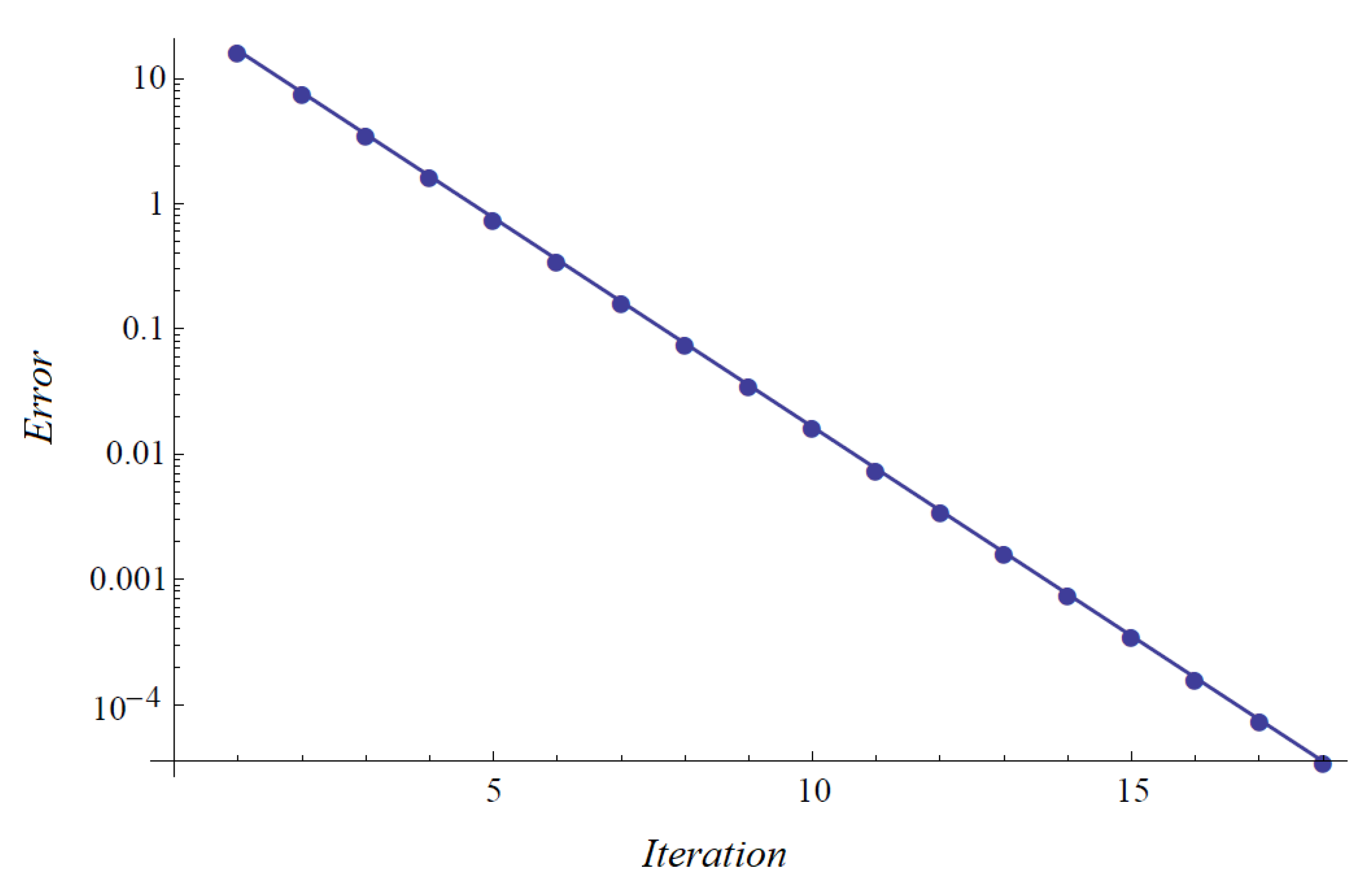
Example 3.

Consider the matrix equation

$$X=Q+A_1^{\ast }X{A}_1+A_2^{\ast }X{A}_2,$$

(29)

where $Q,A_1$ and $A_2$ are given by

$$Q=\left(\begin{array}{cccc}9& 3& 1& 1\\ 3& 9& 3& 1\\ 1& 3& 9& 3\\ 1& 1& 3& 9\end{array}\right),A_1=\left(\begin{array}{cccc}0.0325& 0.057& 0.057& 0.0325\\ 0.057& 0.0325& 0.0325& 0.057\\ 0.057& 0.0325& 0.0325& 0.057\\ 0.0325& 0.057& 0.0325& 0.057\end{array}\right),$$

$$A_2=\left(\begin{array}{cccc}0.68& 0.0871& 0.68& 0.0871\\ 0.0871& 0.68& 0.0871& 0.68\\ 0.68& 0.0871& 0.68& 0.0871\\ 0.0871& 0.68& 0.0871& 0.68\end{array}\right).$$

Define $\mathsf{\Theta }\left(t\right)=t+1$ and $\mathcal{F}\left(X\right)=\frac{X}{8}$. Then, conditions (a) and (b) of Theorem 14 are satisfied for $M=2$. By using the iterative sequence,

$$X_{n+1}=Q+\sum _{i=1}^2{A}_i^{\ast }{X}_n{A}_i$$

with

$$X_0=\left(\begin{array}{cccc}0& 0& 0& 0\\ 0& 0& 0& 0\\ 0& 0& 0& 0\\ 0& 0& 0& 0\end{array}\right).$$

After 18 iterations, we get the unique solution

$$\widehat{X}=\left(\begin{array}{cccc}16.774& 3.03286& 1.87143& 1.00872\\ 3.03286& 16.774& 3.02615& 1.87143\\ 1.87143& 3.02615& 16.774& 3.03286\\ 1.00872& 1.87143& 3.03286& 16.774\end{array}\right)$$

of the matrix Equation (29). The residual error is $R_{18}=\left|\right|\widehat{X}-{\displaystyle \sum _{i=1}^2}{A}_i^{\ast }\widehat{X}{A}_i\left|\right|=3.50316\times {10}^{-5}$ and the convergence history is given in the Figure 1:

6. Conclusions

This paper is concerned with the existence and uniqueness of the best proximity point results for $\acute{C}$iri$\acute{c}$ type contractive conditions via auxiliary functions $\psi \in \mathsf{\Psi }$ and $\mathsf{\Theta }\in \mathsf{\Omega }$ in the framework of complete metric spaces and complete partially ordered metric spaces. In addition, as a consequence, some fixed point results as a special case of our best proximity point results of the relevant contractive conditions in such spaces are studied. To illustrate the existence results, some examples are constructed. Finally, as an application of our fixed point result for partially ordered metric space, the existence of positive definite solution for nonlinear matrix equation is investigated and a numerical example is presented. Our results generalized the results of Jleli et al. [4,32], Suzuki [33] and Nieto et al. [39].

References

- Banach, S. Sur les opérations dans les ensembles abstraits et leur application aux-equations intégrales. Fundam. Math. 1922, 3, 133–181. [Google Scholar] [CrossRef]
- Hussain, N.; Kutbi, M.A.; Salimi, P. Fixed point theory in α-complete metric spaces with applications. Abstr. Appl. Anal. 2014, 2014, 280817. [Google Scholar] [CrossRef]
- Hussain, N.; Parvaneh, V.; Samet, B.; Vetro, C. Some fixed point theorems for generalized contractive mappings in complete metric spaces. Fixed Point Theory Appl. 2015, 2015, 185. [Google Scholar] [CrossRef]
- Jleli, M.; Samet, B. A new generalization of the Banach contraction principle. J. Inequal. Appl. 2014, 2014, 38. [Google Scholar] [CrossRef] [Green Version]
- Samet, B.; Vetro, C.; Vetro, P. Fixed point theorem for α-ψ-contractive type mappings. Nonlinear Anal. 2012, 75, 2154–2165. [Google Scholar] [CrossRef]
- Salimi, P.; Latif, A.; Hussain, N. Modified α-ψ-contractive mappings with applications. Fixed Point Theory Appl. 2013, 2013, 151. [Google Scholar] [CrossRef]
- Hussain, N.; Kutbi, M.A.; Khaleghizadeh, S.; Salimi, P. Discussions on recent results for α-ψ-contractive mappings. Abstr. Appl. Anal. 2014, 2014, 456482. [Google Scholar] [CrossRef]
- Ahmad, J.; Al-Mazrooei, A.E.; Cho, Y.J.; Yang, Y.O. Fixed point results for generalized Θ-contractions. J. Nonlinear Sci. Appl. 2017, 10, 2350–2358. [Google Scholar] [CrossRef]
- Liu, X.D.; Chang, S.; Xiao, Y.; Zhao, L.C. Existence of fixed points for Θ-type contraction and Θ-type Suzuki contraction in complete metric spaces. Fixed Point The. Appl. 2016, 2016, 8. [Google Scholar] [CrossRef]
- Parvaneh, V.; Golkarmanesh, F.; Hussain, N.; Salimi, P. New fixed point theorems for α-HΘ-contractions in ordered metric spaces. J. Fixed Point Theory Appl. 2016, 18, 905–925. [Google Scholar] [CrossRef]
- Abbas, M.; Hussain, A.; Kumam, P. A coincidence best proximity point problem in G-metric spaces. Abstr. Appl. Anal. 2015, 2015, 243753. [Google Scholar] [CrossRef]
- Abkar, A.; Gabeleh, M. Best proximity points for cyclic mappings in ordered metric spaces. J. Optim. Theory Appl. 2011, 150, 188–193. [Google Scholar] [CrossRef]
- Abkar, A.; Gabeleh, M. The existence of best proximity points for multivalued non-self-mappings. Rev. Acad. Cienc. Exactas Fis. Nat. Ser. A Math. 2013, 107, 319–325. [Google Scholar] [CrossRef]
- Ali, M.U.; Kamran, T.; Shahzad, N. Best proximity point for α-ψ-proximal contractive multimaps. Abstr. Appl. Anal. 2014, 2014, 181598. [Google Scholar] [CrossRef]
- Amini-Harandi, A. Best proximity points for proximal generalized contractions in metric spaces. Optim. Lett. 2013, 7, 913–921. [Google Scholar] [CrossRef]
- Amini-Harandi, A.; Fakhar, M.; Hajisharifi, H.R.; Hussain, N. Some new results on fixed and best proximity points in preordered metric spaces. Fixed Point Theory Appl. 2013, 2013, 263. [Google Scholar] [CrossRef] [Green Version]
- Basha, S.S. Discrete optimization in partially ordered sets. J. Glob. Optim. 2012, 54, 511–517. [Google Scholar] [CrossRef]
- Choudhurya, B.S.; Maitya, P.; Metiya, N. Best proximity point results in set-valued analysis. Nonlinear Anal. Model. Control 2016, 21, 293–305. [Google Scholar]
- Eldred, A.; Veeramani, P. Existence and convergence of best proximity points. J. Math. Anal. Appl. 2006, 323, 1001–1006. [Google Scholar] [CrossRef] [Green Version]
- Hussain, A.; Adeel, M.; Kanwal, T.; Sultana, N. Set Valued Contraction of Suzuki-Edelstein-Wardowski Type and Best Proximity Point Results. Bull. Math. Anal. Appl. 2018, 10, 53–67. [Google Scholar]
- Hussain, N.; Latif, A.; Salimi, P. Best proximity point results for modified Suzuki α-ψ-proximal contractions. Fixed Point Theory Appl. 2014, 2014, 10. [Google Scholar]
- Hussain, N.; Kutbi, M.A.; Salimi, P. Best proximity point results for modified α-ψ-proximal rational contractions. Abstr. Appl. Anal. 2013, 2013, 927457. [Google Scholar]
- Khan, A.R.; Shukri, S.A. Best proximity points in the Hilbert ball. J. Nonlinear Convex Anal. 2016, 17, 1083–1094. [Google Scholar]
- Karapinar, E. Best proximity points of cyclic mappings. Appl. Math. Lett. 2007, 335, 79–92. [Google Scholar]
- Komal, S.; Sultana, N.; Hussain, A.; Kumam, P. Optimal Approximate Solution for Generalized Contraction Mappings. Commun. Math. Appl. 2016, 7, 23–36. [Google Scholar]
- Latif, A.; Abbas, M.; Husain, A. Coincidence best proximity point of Fg-weak contractive mappings in partially ordered metric spaces. J. Nonlinear Sci. Appl. 2016, 9, 2448–2457. [Google Scholar]
- Latif, A.; Hezarjaribi, M.; Salimi, P.; Hussain, N. Best proximity point theorems for α-ψ-proximal contractions in intuitionistic fuzzy metric spaces. J. Inequal. Appl. 2014, 2014, 352. [Google Scholar]
- Lo’lo, P.; Vaezpour, S.M.; Esmaily, J. Common best proximity points theorem for four mappings in metric-type spaces. Fixed Point Theory Appl. 2015, 2015, 47. [Google Scholar]
- Ma, Z.; Jiang, L.; Sun, H. C*-algebra-valued metric spaces and related fixed point theorems. Fixed Point Theory Appl. 2014, 2014, 206. [Google Scholar]
- Ma, Z.; Jiang, L. C*-algebra-valued b-metric spaces and related fixed point theorems. Fixed Point Theory Appl. 2015, 2015, 111. [Google Scholar]
- Zhang, J.; Su, Y.; Cheng, Q. A note on—A best proximity point theorem for Geraghty-contractions. Fixed Point Theory Appl. 2013, 2013, 99. [Google Scholar]
- Jleli, M.; Samet, B. Best proximity points for α-ψ-proximal contractive type mappings and applications. Bull. Sci. Math. 2013, 137, 977–995. [Google Scholar]
- Suzuki, T. The existence of best proximity points with the weak P-property. Fixed Point Theory Appl. 2013, 2013, 259. [Google Scholar] [Green Version]
- Abkar, A.; Gabeleh, M. Generalized cyclic contractions in partially ordered metric spaces. Optim. Lett. 2012, 6, 1819–1830. [Google Scholar]
- Basha, S.S. Best proximity point theorems on partially ordered sets. Optim. Lett. 2013, 7, 1035–1043. [Google Scholar]
- Pragadeeswarar, V.; Maruda, M. Best proximity points: Approximation and optimization in partially ordered metric spaces. Optim. Lett. 2013, 7, 1883–1892. [Google Scholar]
- Pragadeeswarar, V.; Marudai, M. Best proximity points for generalized proximal weak contractions in partially ordered metric spaces. Optim. Lett. 2015, 9, 105–118. [Google Scholar]
- Pragadeeswarar, V.; Marudai, M.; Kumam, P. Best proximity point theorems for multivalued mappings on partially ordered metric spaces. J. Nonlinear Sci. Appl. 2016, 9, 1911–1921. [Google Scholar] [Green Version]
- Nieto, J.T.; Rodríguez-López, R. Contractive Mapping Theorems in Partially Ordered Sets and Applications to Ordinary Differential Equations. Order 2005, 22, 223–239. [Google Scholar]
- Ran, A.C.M.; Reurings, M.C.B. A fixed point theorem in partially ordered sets and some applications to matrix equations. Proc. Am. Math. Soc. 2003, 132, 1435–1443. [Google Scholar]
Figure 1.
Convergence history for (29).
© 2019 by the authors. Licensee MDPI, Basel, Switzerland. This article is an open access article distributed under the terms and conditions of the Creative Commons Attribution (CC BY) license (http://creativecommons.org/licenses/by/4.0/).
Share and Cite
MDPI and ACS Style
Ma, Z.; Hussain, A.; Adeel, M.; Hussain, N.; Savas, E. Best Proximity Point Results for Generalized Θ-Contractions and Application to Matrix Equations. Symmetry 2019, 11, 93. https://0-doi-org.brum.beds.ac.uk/10.3390/sym11010093
AMA Style
Ma Z, Hussain A, Adeel M, Hussain N, Savas E. Best Proximity Point Results for Generalized Θ-Contractions and Application to Matrix Equations. Symmetry. 2019; 11(1):93. https://0-doi-org.brum.beds.ac.uk/10.3390/sym11010093
Chicago/Turabian StyleMa, Zhenhua, Azhar Hussain, Muhammad Adeel, Nawab Hussain, and Ekrem Savas. 2019. "Best Proximity Point Results for Generalized Θ-Contractions and Application to Matrix Equations" Symmetry 11, no. 1: 93. https://0-doi-org.brum.beds.ac.uk/10.3390/sym11010093
Note that from the first issue of 2016, this journal uses article numbers instead of page numbers. See further details here.