No-Reference Image Quality Assessment with Local Gradient Orientations


Department of Computer and Control Engineering, Rzeszow University of Technology, W. Pola 2, 35-959 Rzeszow, Poland
Symmetry 2019, 11(1), 95; https://0-doi-org.brum.beds.ac.uk/10.3390/sym11010095
Submission received: 22 December 2018
/
Revised: 12 January 2019
/
Accepted: 13 January 2019
/
Published: 16 January 2019
Abstract
:Image processing methods often introduce distortions, which affect the way an image is subjectively perceived by a human observer. To avoid inconvenient subjective tests in cases in which reference images are not available, it is desirable to develop an automatic no-reference image quality assessment (NR-IQA) technique. In this paper, a novel NR-IQA technique is proposed in which the distributions of local gradient orientations in image regions of different sizes are used to characterize an image. To evaluate the objective quality of an image, its luminance and chrominance channels are processed, as well as their high-order derivatives. Finally, statistics of used perceptual features are mapped to subjective scores by the support vector regression (SVR) technique. The extensive experimental evaluation on six popular IQA benchmark datasets reveals that the proposed technique is highly correlated with subjective scores and outperforms related state-of-the-art hand-crafted and deep learning approaches.
The recent advancement of digital imaging has stimulated a tremendous growth in the use of visual information for communication [1,2,3]. Therefore, it is essential to develop reliable automatic image quality assessment (IQA) measures for the evaluation of results of image processing methods for the acquisition, storage, transmission, restoration, or enhancement. The main role of IQA measures is to provide the objective assessment and replace cumbersome tests with human subjects [4]. The IQA measures are divided into three categories, based on the availability of reference images [1,5,6]: full-reference (FR), reduced-reference (RR), and no-reference (NR) approaches. In an FR-IQA measure, a distorted image is compared with its reference image, while only some statistics of the distortion-free image are available in the RR-IQA case. The peak signal-to-noise ratio (PSNR) is often used as an FR-IQA model due to its simplicity. However, it weakly correlates with human perception [5]. Therefore, more suitable measures have been developed that employ structural information [7], image statistical properties [8], visual saliency maps [9,10], structure and contrast changes [11], phase congruency [12], distortion distribution [13], or other measures [14,15]. The RR-IQA measures use only a part of reference data [16].
In this work, the discussion is confined to NR approaches, which are considered challenging and highly desired due to their applicability in absence of reference images. Many measures are devoted to evaluating the perceptual quality of images distorted by Gaussian white noise, JPEG compression, contrast change, or Gaussian blur [17,18]. Since their practical application is limited and based on the prior knowledge of distortion types, general-purpose NR methods have been developed. Many of them assume that statistical regularities of natural images can be reflected by natural scene statistics (NSS), as the Human Visual System (HVS) is very sensitive to local regularities [19]. Consequently, NSS characteristics of distorted images are used for the IQA in many domains, e.g., Discrete Cosine Transform (DCT) [20], wavelet [21,22], or spatial [23]. A variety of gradient-based features are often employed to model NSS [24]. Furthermore, the use of perceptual features [25,26,27] or image patches [28] can be found in the literature.Since the supervised learning bridges image statistics with the perceptual quality, it is often applied to obtain a model used for the quality prediction. For the learning, the Support Vector Regression (SVR) [20,21,23,27], neural networks [24], or random forests [29] are applied. In methods that do not use supervised learning, distortion types are modeled with a set of centroids of quality levels or NSS from multiple cues [30,31]. Another direction is to employ a pseudo-reference image which is created and compared with a distorted image with blockiness, sharpness, and noisiness metrics [32]. Recently, many NR-IQA approaches which use deep neural network (DNN) architectures have been introduced. They merge the feature extraction and quality prediction steps. However, they suffer from a small number of training examples available in IQA benchmark datasets or use complex architectures that are devoted to image recognition tasks. To overcome these limitations, most of them use image patches [33,34], train models using FR-IQA measures instead of subjective scores [34,35], or perform fine-tuning to adopt an architecture to the IQA [36]. Interestingly, some DNN-based approaches use features introduced in earlier methods [35].
The HVS is sensitive to local structures, which are often described using local binary patterns (LBP) and gradient-based statistics. However, a spatial distribution of LBP may not be able to capture more complex structures [37]. Thus, statistics extracted from gradient maps often occur in conjunction with other approaches to improve the IQA performance [27,38]. Such techniques use global distributions of gradient magnitude maps [25], relative gradient orientations or magnitude [24,39].
To describe an image and efficiently take into account local gradient orientations, Histogram of Oriented Gradients (HOG) descriptor can be used [40]. However, the HOG produces high-dimensional feature vectors, which are devoted to object recognition tasks due to their discriminative capabilities. Consequently, considering its application to the IQA, it is worth noticing that an original image content of an assessed image, which is described using the HOG, may influence the quality prediction performance. The descriptor also strongly depends on the size of processed image blocks and the described neighborhood. Since the image gradient orientation captured by the HOG and its relevance for the NR-IQA is interesting and still seems largely uninvestigated, in this paper, a novel no-reference technique for the image quality assessment with a SEt of Histogram of OriEnted GRadients (HOG) descriptors [40] (SEER) is introduced. In the SEER, in contrary to a widely accepted application of the HOG, an image is described by a set of descriptors which are obtained taking into account different local neighborhoods. In other words, each feature vector is composed of histograms of gradient orientations calculated for image regions (cells), which are arranged together with their neighboring cells in blocks. The descriptors in the set consider different sizes of image regions and blocks. Then, each descriptor is characterized by a histogram, seen as perceptual features. In a typical image recognition system, high-dimensional descriptors are often compared with each other. However, to apply the HOG to the NR-IQA, such comparison cannot take place since a distortion-free image and its descriptors are unavailable. Furthermore, the feature vectors in the HOG are designed to discriminate objects in images. Therefore, in the SEER, to train the SVR model, statistics of descriptors are employed instead of high-dimensional vectors. To improve the IQA performance, the method processes luminance and chrominance channels of an image, as well as their high-order derivatives.
The extensive experimental evaluation of the introduced NR measure against the related state-of-the-art techniques on six popular large-scale IQA benchmark datasets, which contain various distortion types, demonstrates that the SEER provides the higher quality prediction accuracy than compared NR models and is consistent with subjective scores. The method was evaluated against hand-crafted and deep learning NR measures.
The rest of this paper is arranged as follows. Section 1 reviews previous work on NR-IQA and Section 2 describes the proposed measure. Section 3 presents and discusses the experimental results obtained for the SEER and the related measures on TID2013 [41], TID2008 [42], CSIQ [43], LIVE [7], and LIVE In the Wild Image Quality Challenge (LIVE WIQC) [44] datasets. Finally, Section 4 concludes the paper.
1. Related Work
In this section, a brief review of previous studies closely related to the introduced work is presented.
The introduced SEER is based on gradient processing. However, there are many works which employ other features. For example, Moorthy and Bovik proposed a two-stage framework, in which distortion type is predicted and then an image is evaluated [21]. Saad et al. trained a probabilistic model with DTC-based NSS as a single-stage framework [20]. The generalized Gaussian distribution used for capturing NSS with locally normalized luminance coefficients is employed in Blind/Referenceless Image Spatial QUality Evaluator (BRISQUE) [23]. A scheme which combines artifact-specific metrics and employs a generalized Laplace distribution of the difference of two adjacent pixel values in an image was introduced by Fang et al. [45]. The measure uses three transductive k-nearest neighbor algorithms to map the metrics into subjective scores. Normalized gradients magnitude and Laplacian of Gaussian responses were jointly used by Xue et al. [25]. Le et al. [46], in turn, used a histogram of local binary patterns (LBP) obtained for a gradient map. They also used LBP extracted from texture and structural maps [38]. A more advanced gradient-based image descriptor, Speeded-Up Robust Features (SURF), is employed in the measure proposed by Oszust [27]. In that work, the sample mean, standard deviation, entropy, skewness, kurtosis, and histogram variance for the assessed image, the image filtered with Prewitt operators, and their SURF features are used. In Optimized filteRing with binAry desCriptor for bLind imagE quality assessment technique (ORACLE) [47], in turn, a data-driven filtering based on the appearance of Features From Accelerated Segment Test (FAST) in grayscale images is proposed. The histograms of Fast Retina Keypoint (FREAK) descriptors for keypoints detected in filtered images are used to characterize the assessed content. The sample mean, standard deviation, and histogram variance of raw local patches describing FAST keypoints in images filtered with the bilaplacian operator in the YCbCr color space are used in stATistics of pixel blocks of local fEatuRes (RATER) measure [48]. Unlabeled data for learning Gabor features and modeling an image using the soft-assignment coding with the max pooling are employed in [49]. In another method that uses a codebook, High Order Statistics Aggregation (HOSA) [28], K-means clustering of normalized image patches and their description with the low and high order statistics are considered. The HOSA uses the soft assignment for an image representation and trains the SVR model for the prediction. Screen content images were assessed by Lu and Li [50] using orientation selectivity mechanism for extraction of orientation features.
Gradient-based techniques are often employed to provide effective IQA measures [11,24,25,46]. These measures use global distributions of gradient magnitude maps [25], relative gradient orientations or magnitude [24,39]. For example, in the Oriented Gradients Image Quality Assessment (OG-IQA) index, in which a correlation structure of image gradient orientations [24] is employed to train a quality model with AdaBoosting-backpropagation neural network. In that work, histograms of gradient magnitude, relative gradient orientation, and relative gradient magnitude maps are used and characterized using the histogram variance. These gradient-based measures do not take into account local gradient distributions. Such distributions are used in the HOG to provide a feature vector composed of 1-D histograms of gradient directions of pixels within image regions (cells) [40]. In the literature, there are FR-IQA measures which compare a reference image with the distorted image, calculating a distance between corresponding HOG vectors [51] or produce a weight map for the FR SSIM index [52]. In the technique proposed by Ahn et al. [18], in turn, blurred images are assessed by comparing HOG vectors approximated by a random sample consensus set (RANSAC).
Taking into account the referred works, it can be stated that the effectiveness of the HOG in NR image quality prediction remains largely uninvestigated, and a promising application of this descriptor to the NR-IQA is introduced for the first time in this paper.
2. Proposed NR Measure
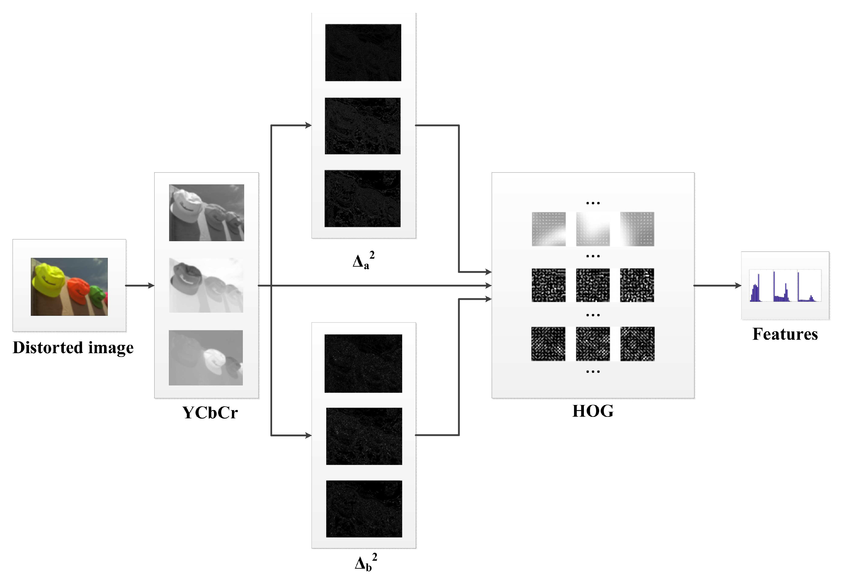
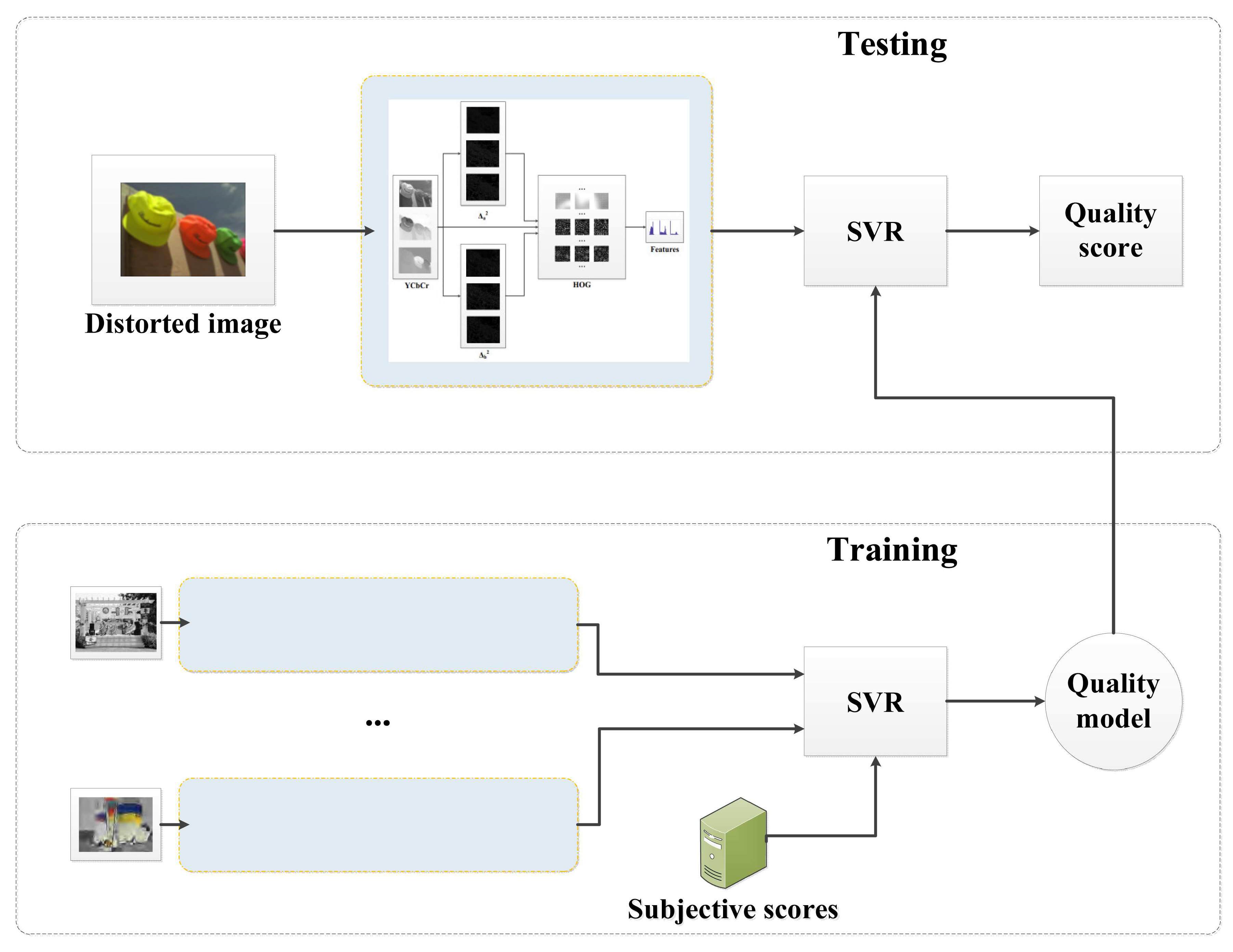
In this section, the feasibility of using the HOG for the NR-IQA is investigated. The image processing steps in the SEER are explained in details in Figure 1, while in Figure 2 the block diagram of the proposed method is shown. As illustrated, the measure uses the HOG and provides feature vectors for luminance and chrominance channels of a distorted image, as well as for channels filtered using two bilaplacian operators. The measure uses differently sized image regions and the way the regions are combined together in the HOG descriptors. In the SEER, the K HOG features are obtained for each channel and their histograms are used to train a quality prediction model.
2.1. Local Gradient Orientations
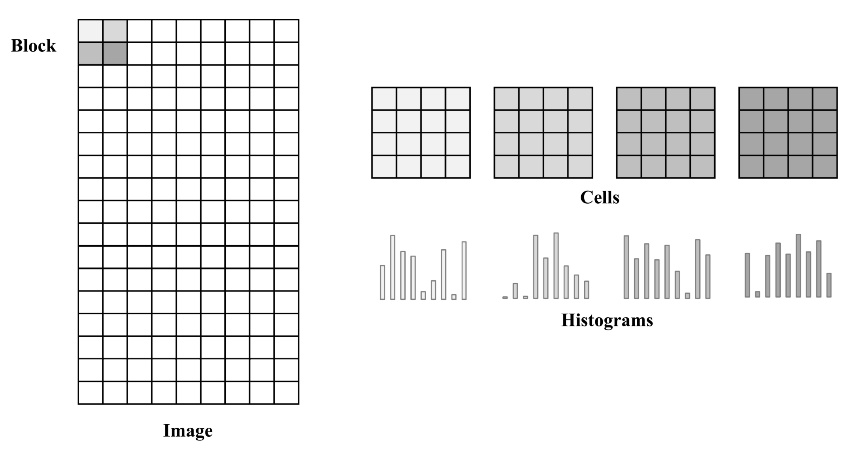
The HVS is sensitive to variations in local structures [19,39]. Such sensitivity and the resultant subjective perception of an image are related to local semantic structural information which forms primitives in V1 [39]. Local distributions of gradients are used in the HOG to characterize an image [40]. Specifically, a 2D image I is convolved with 1-D Prewitt filters in the horizontal () and vertical () directions to obtain gradients. Then, the edge magnitude is calculated as , and its orientation is obtained as . The orientation is then transformed to degrees range, ensuring that the opposite directions are assigned the same angle. The I is divided into adjacent, non-overlapping cells of size and, for each cell, the gradient orientations are binned into o bins with votes based on their magnitudes. To reduce aliasing, each pixel contributes to adjacent bins a fraction of its gradient magnitude. To reduce contrast changes, in turn, histograms for cells are normalized. Since gradient magnitudes carry the information about the described object in a region, to preserve the information, cells are grouped into overlapping blocks. There are cells in each block. Then, cell histograms are concatenated and normalized using -norm. Finally, the obtained features for blocks are concatenated and normalized. This normalization makes the descriptor invariant against overall image contrast [40]. The division of an image into blocks and cells is shown in Figure 3. The number of overlapping cells between adjacent blocks is equal to , where . The number of dimensions in the resulting feature vector D is calculated as:
where M and N denote the height and width of an image, respectively. If is equal to , or to , the length of the vector is calculated without the subtraction in the denominator. For an exemplary image , the lengths of the feature vectors for the descriptors and , calculated with , are 2,340,900 and 580,644, respectively. Such high-dimensional feature vectors are designed for robust object recognition and they cannot be used to train a quality model with the SVR. Therefore, it is shown in this paper that their histograms are sensitive to image degradation, consequently leading to the efficient application of the HOG to the NR-IQA.
2.2. Feature Extraction
In the introduced NR measure, a distorted RGB image is converted to the YCbCr color space. The YCbCr color space is specified in ITU-R BT.601 and selected as the preferred format for video broadcasting with the efficient use of the channel bandwidth [53]. Following the finding that the image filtering can enhance the image quality prediction of NR-IQA measures [47] and the bilapacian operator can be used to capture more information about described image regions for the IQA than it can be achieved with other filters [48], the SEER uses the YCbCr color space and filters color channels of the assessed image with two bilaplacian kernels and . The bilaplacian is obtained by convolving two Laplacian kernels. The following kernels are used:
Finally, and , where “*” denotes the convolution. Consequently, a filtered channel (e.g., ) is obtained using the convolution .
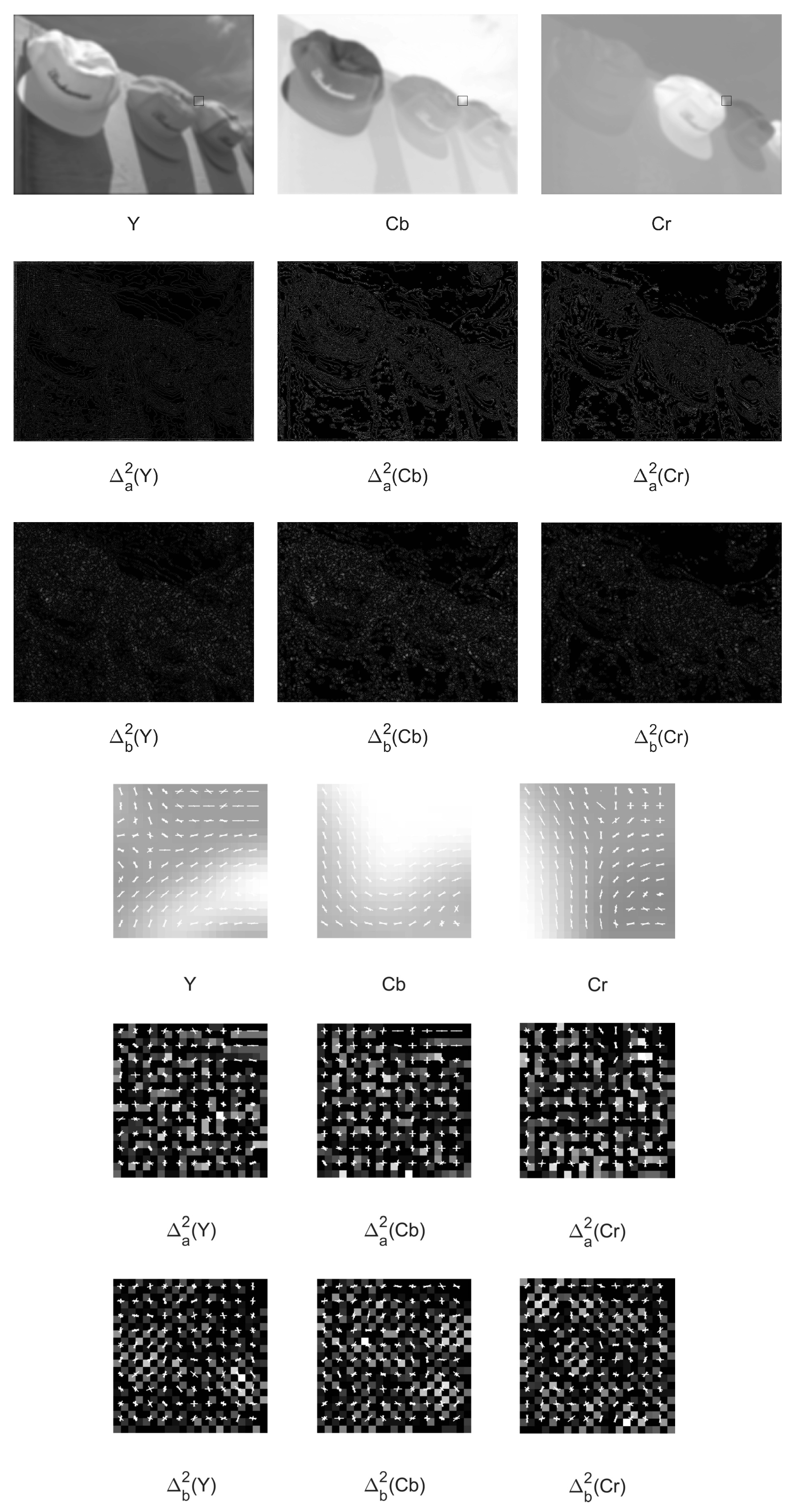
To show that the HOG technique provides different feature vectors for YCbCr components, Figure 4 presents an exemplary distorted image and the visualization of the HOG obtained for a small square image patch. For the visualization, a grid of rose plots is used. In the grid, each rose expresses the distribution of gradient orientations within a cell. The length of a petal indicates the contribution of a given orientation within the cell histogram and displays two times o petals. As presented, the feature vectors for the descriptor have different shapes for different YCbCr channels. The figure also contains image patches filtered with two used bilaplacian operators and .
As shown in Figure 4, the differences between descriptors for channels seem to justify the need for their joint application in order to extract more information about the described image regions. Furthermore, since the size of a local structure in an image cannot be determined in advance, the method uses several HOG descriptors with cells and blocks of different sizes. The HOG descriptor produces high-dimensional features, depending on its focus on a local appearance of objects within an image. Thus, in this paper, each obtained feature vector is characterized using its histogram . The histogram is used since it captures distributions of natural images [24]. The values in the feature vectors for images are in the range . Therefore, the number of bins in the histogram and its variance is calculated by dividing the range into d intervals and using them for the determination of bin centers.
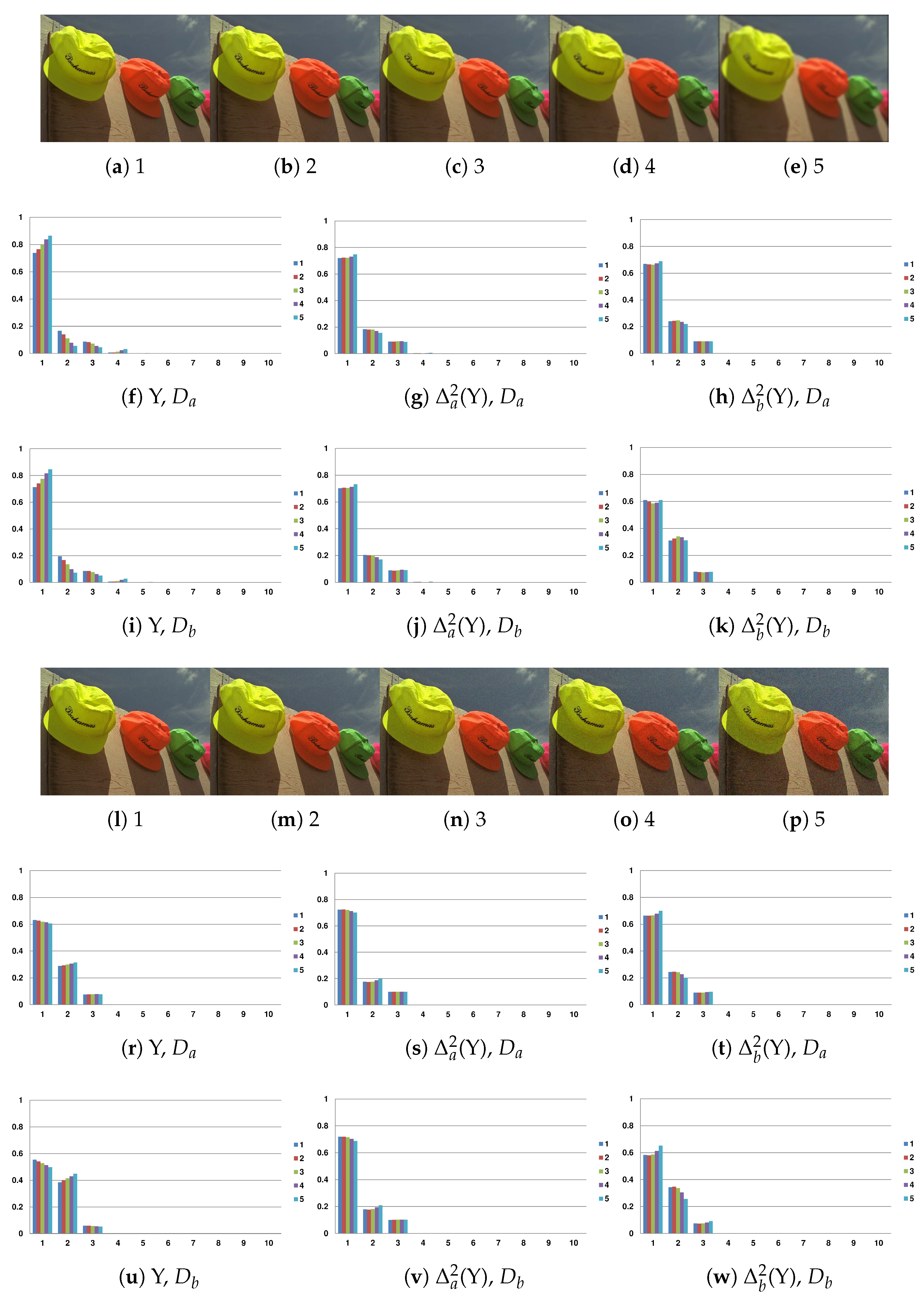
To illustrate that the used statistics can characterize the distortion severity of images, they are computed for two sequences of images distorted with Gaussian blur and Gaussian noise [41]. Here, the descriptors and are used. For the computation of the histogram, 10 bins are applied. As shown in Figure 5, the histogram responds consistently to the distortion type and its severity.
In the SEER, for YCbCr channels and channels filtered with two bilaplacian operators, feature vectors for the HOG descriptors are obtained and concatenated. This can be written as , , , , , , or , where . There are nine HOG descriptors per ith image, with different C and B. Hence, the HOG descriptors for the I can be written as , , . Finally, the perceptual feature vector is obtained as , , , ,. The parameters of HOG descriptors used in the SEER are discussed in details in Section 3.6. Since the distortions affect images across scales [23], the method also processes an input image which is downsampled by a factor of two to improve the quality prediction. Finally, the concatenated histograms for an input image and its downscaled version are used to train the SVR model. The SVR model which maps the vector into subjective ratings is obtained using LIBSVM library [54]. Here, as in many NR techniques [24,46], the radial basis function (RBF) kernel is employed. Finally, given an input image, the model predicts its quality and provides the objective score Q.
3. Experimental Results and Discussion
3.1. Datasets and Protocol
In this work, to evaluate an NR metric, six publicly available large IQA datasets were used: TID2013 [41], TID2008 [42], CSIQ [43], LIVE [7], LIVE WIQC [44], and the Waterloo Exploration Database (WE) [55]. The first four datasets are typically selected to evaluate recently introduced measures [34,56,57], while the WE dataset, similar to the Group MAD Competition [58,59], is tied with a novel evaluation methodology. The LIVE WIQC dataset contains subjective scores collected in an uncontrolled manner using the Amazon Mechanical Turk. However, it contains images captured with a mobile camera and can be used for the evaluation of NR measures using real images. The TID2013 dataset is the largest and the most demanding public IQA benchmark. It consists of 3000 distorted images and covers 24 image distortion types. The other datasets contain only half (TID2008) or less than one-third of the number of the images in TID2013 (CSIQ and LIVE). The LIVE dataset contains popular distortions, such as JPEG compression, JPEG2000 compression, Gaussian blur, white noise, or simulated fast fading Rayleigh channel. It is worth noticing that some distortion types in TID2013 can be regarded as multiple, e.g., lossy compression of noisy images. Interestingly, most existing general-purpose NR measures are designed to provide an acceptable performance on the LIVE [32]. As shown in Section 3.3, some of them experience a drop in the performance on datasets that contain more diverse distortions. The datasets contain high-quality images, their distorted images, and related subjective scores. The subjective scores obtained in tests with human subjects are denoted as mean opinion scores (MOS) or differential MOS (DMOS). The WE dataset contains images distorted with JPEG compression, JPEG2000 compression, white Gaussian noise, and Gaussian blur. However, it does not contain subjective scores. The datasets are characterized in Table 1.
To measure the consistency of the prediction results provided by an IQA measure with subjective ratings, the following four indices were considered [60]: the Spearman’s Rank Correlation Coefficient (SRCC), Kendall Rank order Correlation Coefficient (KRCC), Pearson linear Correlation Coefficient (PCC), and Root Mean Square Error (RMSE). PCC and RMSE were calculated after a nonlinear mapping between the vectors of objective and subjective scores, and (MOS or DMOS), respectively. For the mapping, the following function was used [60]: where are parameters of the fitted regression model, Q is the objective score, and is the fitted score.
The evaluation protocol associated with the WE dataset requires: the calculation of pristine/distorted image discriminability test (D-test), listwise ranking consistency test (L-test), and pairwise preference consistency test (P-test) [55]. The D-test uses predictions of a model to classify distorted and pristine images. Larger values of D denote better separability. The L-test, in turn, adopts the average SRCC to quantify the ranking consistency among distorted images. Finally, the P-test compares preference predictions of IQA models on pairs of images whose quality is clearly discriminable [55], dividing the number of image pairs with correctly predicted concordance by the number of image pairs. The values obtained in tests lie in .
3.2. Model Training
The proposed method should be trained to obtain the SVR model used for the quality prediction. Therefore, a typical protocol used for the validation of NR techniques was adopted, in which each image dataset was divided into disjoint training and testing subsets, i.e., distorted images of 80% reference images were used in training and the remaining 20% of images were used for testing [28,32,46]. Then, to avoid bias and fairly compare a measure with other measures, the performance of each method was reported in terms of the median values of SRCC, KRCC, PCC, and RMSE over 100 training-testing iterations [61].
3.3. Performance on Individual Datasets
The performance of the presented NR measure was compared with those of the related state-of-the-art techniques. The following NR measures were considered: (i) HOSA [28]; (ii) BPRI [32]; (iii) BRISQUE [24]; (iv) IL-NIQE [31]; (v) SISBLIM [62]; (vi) OG-IQA [24]; (vii) GWH-GLBP [46]; and (viii) RATER [48]. Among NR measures, which, to some extent, are similar to the SEER, the RATER, HOSA, and IL-NIQE assess color images, while the OG-IQA incorporates image gradients. The GWH-GLBP and SISBLIM are designed for the evaluation of images with multiple distortions. The RATER and BPRI are recently introduced general-purpose measures. However, due to distortion-specific steps in BPRI, its range of applicability is larger than those of distortion-specific measures, but it seems to be confined to several distortion types. As reported by Zhang et al., the IL-NIQE is superior to the BLIINDS2, DIIVINE, CORNIA, NIQE, BRISQUE, and QAC [31]. The HOSA, in turn, is reported to outperform the GM-LOG, BRISQUE, or IL-NIQE [28].
The experimental evaluation was conducted on five IQA datasets using the protocol shown in Section 3.1. For the fair comparison, the parameters of all learning-based techniques were obtained aiming at their best performance [25,31]. The methods were run using publicly available implementations. For the SVR, the popular LIBSVM library was used [54]. The parameters of AdaBoosting BP neural network in the OG-IQA were also determined. The methods that do not require training (BPRI, IL-NIQE, and SISBLIM) were evaluated using the defined testing subsets of images in datasets. The SEER was run with o = 36 and d = 30 (see Section 3.6).
Table 2 summarizes the results on IQA datasets, where the best result for each performance index is written in bold. The table also contains average values for SRCC, KRCC, and PCC. The RMSE was not averaged due to the different range of values in the benchmarks.
As demonstrated, the introduced NR measure outperformed the state-of-the-art measures on four IQA benchmarks, i.e., the TID2013, TID2008, CSIQ, and LIVE. In the case of the LIVE WIQC dataset, the RATER and BRISQUE were slightly better than SEER, which was the third-best measure. Remarkably, the proposed measure had the highest average performance across the datasets, which confirms its usability.
To determine whether the relative performance differences between the measures are statistically significant, the Wilcoxon rank-sum test was used. The test measures the equivalence of the median values of independent samples with a 5% significance level. Here, the null hypothesis assumes that the SRCC values of compared metrics are drawn from a population with equal medians. The results are shown in Table 3, where the symbols “−1”, “0” and “1” denote that the IQA measure in the column was statistically better with a confidence greater than 95%, indistinguishable, or worse than the SEER on a given IQA dataset, respectively. The findings are consistent with conclusions drawn from the previous experiments, i.e., the SEER was statistically better than other measures on the TID2013, TID2008, and LIVE. Taking into account the results for the CSIQ, the SEER was on pair with the RATER, as well as on pair with the RATER and BRISQUE for the LIVE WIQC.
The measures were evaluated using the methodology associated with the WE database [55]. Here, the BRISQUE and HOSA were compared with the SEER. Since the IL-NIQE is reported to provide superior performance using this methodology [55], it is also added to the comparison. The results reported for BRISQUE, HOSA, and IL-NIQE in [55] are presented in Table 4. The SEER, as other techniques, was trained on LIVE dataset. Interestingly, the IL-NIQE, which is much less correlated with subjective scores on LIVE than other measures, yielded encouraging L and P values. This may indicate that the relationship between distortion types, their levels, and used tests in the used methodology may require further attention, leading to its possible improvement. For example, the P values of the measures whose performances on the databases with subjective scores were significantly different seem to be close to its upper limit. Furthermore, the assumption that image quality degrades monotonically with the distortion levels may not be true for all distortion types and content of images, which may influence the results of the L-test [55]. However, it can be seen that all measures provided acceptable performance in the tests on the WE database.
The comparative evaluation of the SEER with state-of-the-art NR methods that use DNN or other neural networks (NN) architectures was based on published results. Due to the large complexity of the models, and the unavailability of learning source codes for some of them, such comparison is very popular. Consequently, many papers report the performance of measures on the basis of results obtained in 10 random training–testing splits on only one or two IQA benchmarks. Furthermore, the coherent comparison of DNN-based methods is often impeded by the exclusion of some distortion types, which can make the use of the largest IQA datasets, such as the TID2013 or TID2008, superfluous. Table 5 contains the comparison of published median values of SRCC and PCC for NN-based NR methods with those obtained for the SEER in 10 training–testing splits. Other performance indices, i.e., KRCC and RMSE, are seldom reported in the referenced works. The results for the TID2008 are not presented since the referenced works were not evaluated on this dataset. As reported, the SEER clearly outperformed other measures on the most demanding datasets, such as the TID2013 or CSIQ. The NN-based measures were better than the SEER on the LIVE dataset. The worse results of the compared models on the datasets that contain considerably more distortions can be attributed to the lack of a sufficient number of training samples or imperfections of used architectures [36,57]. It can be concluded that the introduced hand-crafted NR measure is highly competitive to the recently introduced techniques based on DNN or NN architectures.
3.4. Performance across Datasets
To verify whether the proposed measure is independent of a dataset, a cross-dataset validation was performed. The NR measures were trained on one IQA dataset and tested on the remaining datasets. In the experiment, the learning-based measures were compared on four datasets. The results, in terms of SRCC, reported in Table 6, reveal that the SEER maintained acceptable generalization capability across the datasets. The best results were with bold type. In general, it achieved the best average SRCC.
3.5. Computational Complexity
The computational complexity of a given method was analyzed in terms of the average time taken to assess an image () from the TID2013 dataset. The experiments were performed on a 3.3 GHz Intel Core CPU with 16 GB RAM system running on Microsoft Windows 7 64 bit. For all compared methods, their Matlab implementations were used. As demonstrated in Table 7, the SEER is of moderate complexity. It was faster than IL-NIQE and slower than RATER and HOSA, which also process color images. The execution time of the SEER strongly depends on its parameters. However, unlike other measures, the SEER can be easily run in parallel, since, for the assessed color image, the nine used HOG descriptors were executed for 18 resulting images, including YCbCr color channels, their filtered images, and downsampled images. A simultaneous run of the computation of the HOG for these images using an efficient native implementation (e.g., C++) with a GPU code of the HOG could shorten the execution time of the method up to 162 times.
3.6. Metric Configuration and Contribution of Features
In the SEER, as explained in Section 2.2, an evaluated image is characterized using the histogram of K HOG descriptors. Since the HOG can be used with different parameters, their choice and the resulting IQA performance of the introduced measure requires investigation. SRCC was used as the quality index, taking into account that the remaining criteria similarly indicate the performance of the method.
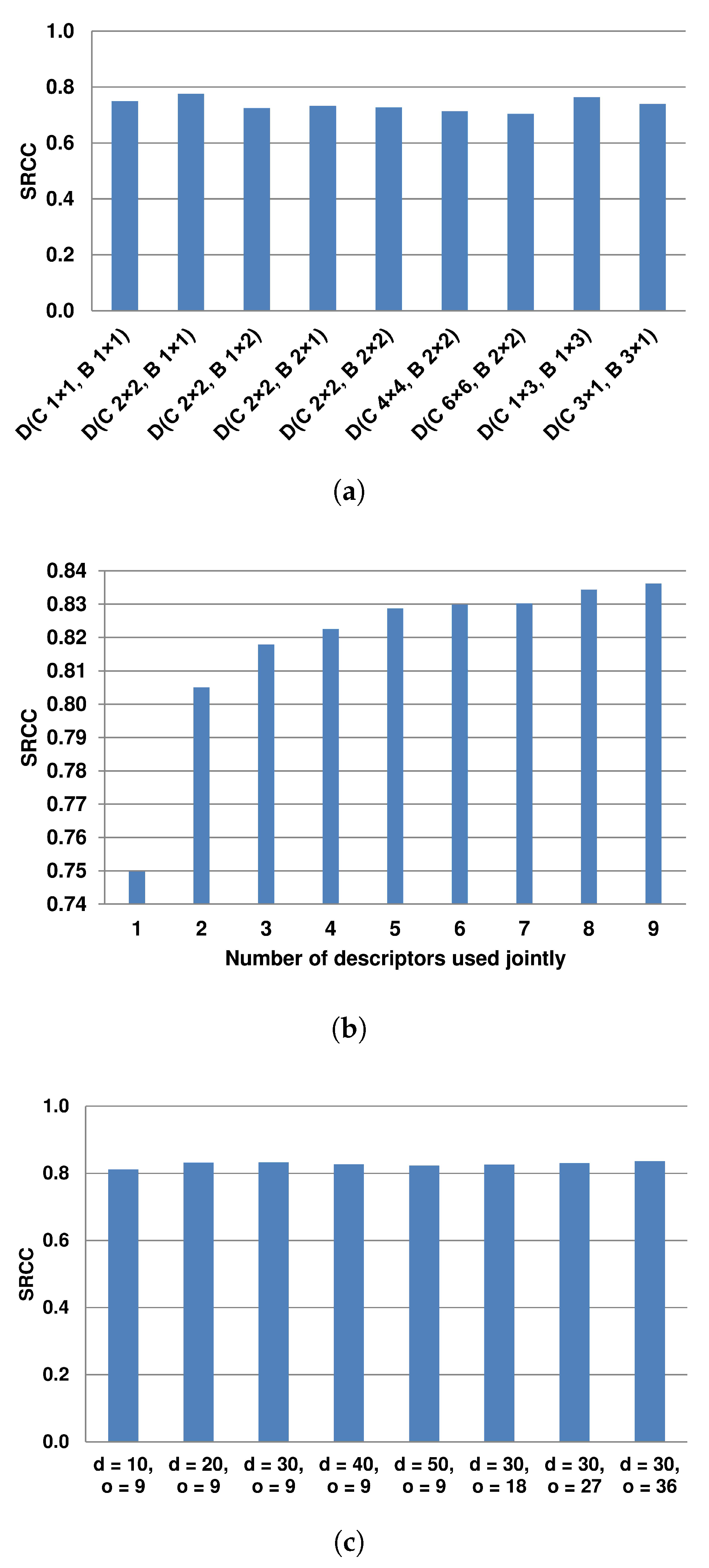
Figure 6a contains SRCC values obtained for the SEER with only one HOG descriptor, using the protocol introduced in the previous section, on the TID2013 dataset. TID2013 was used due to its size and the number of image distortions. In the experiment, the performance of the SEER with many different HOG parameters was investigated. The presented HOG descriptors were run with and . In the IQA, a detailed description of a pixel neighborhood is needed, confirmed by various NR approaches using LBP in which a pixel is characterized by its 8 neighbors. Therefore, HOG configurations with smaller pixel areas were taken into account to determine the IQA performance of the SEER with them. The nine HOG descriptors presented in Figure 6a were selected to be used jointly. In the case of single application of the descriptor , the method resembles approaches in which statistics for a gradient map, among other features, are used for the quality prediction (e.g., [27]). To show that such joint application of the HOG descriptors is beneficial, Figure 6b reports the performance of the method with HOG descriptors. Since the presentation of all possible combinations of these descriptors is unfeasible, the performance is reported for the descriptors added in the order presented in Figure 6a. Interestingly, the SEER with only two HOG descriptors delivered promising performance, outperforming the state-of-the-art measures evaluated in the previous section. It can be assumed that an application of dimensionality reduction or feature selection techniques, which would indicate the most influential descriptors or their statistics, may provide better results. However, these techniques can also deepen the dataset-dependency. Therefore, in this study, the selected HOG descriptors were used in the SEER.
In the proposed method, the descriptors , , and contributed the most to its performance (see Figure 6a). Apart from the size of the cell and the arrangement of cells in the block, the computation of the feature vector in the SEER requires two additional parameters, o and d. Therefore, the performance of the measure was evaluated taking into account their variability. The results in terms of SRCC on the TID2013 are shown in Figure 6c. They reveal that these two parameters almost did not affect the performance of the SEER. In other experiments with the method, and are used.
Since the measure uses YcbCr color space and filtered images, Table 8 presents their contribution to its performance in terms of SRCC on the TID2013. As reported, color channels contributed similarly. However, the channels filtered using the bilaplacian operators carry the most information that can be used for the quality prediction. As reported, the channels alone could not provide satisfactory SRCC performance, which confirms their complementary relationship and justifies their joint application in the SEER.
4. Conclusions
In this work, a novel NR-IQA technique has been presented. The introduced SEER incorporates the distribution of local intensity gradients. The histogram of a set of these descriptors, obtained for YCbCr channels of a distorted image, as well as its channels filtered with bilaplacian operators, are used as perceptual features to train an SVR model for the image quality prediction. It has been shown that the use of a descriptor, which takes into account different sizes of described image regions and their mutual relationship, is beneficial to the IQA, as obtained feature vectors respond consistently to the distortion type and its severity. Furthermore, it has been demonstrated that, to deliver superior performance, the information extracted from YCbCr channels in the bilaplacian domain should be employed. The introduced technique was evaluated and compared with the state-of-the-art NR hand-crafted and NN-based measures on six IQA datasets. The experimental results demonstrate that overall the SEER outperforms the compared NR measures in terms of prediction accuracy and generalization capability.
The future work on the SEER will focus on an application of a keypoint detector that indicates image regions for the description [27,67]. Another promising direction of research is to train a deep learning model using features provided by the SEER, similar to the work in [35].
The Matlab code of the proposed approach is publicly available at http://marosz.kia.prz.edu.pl/SEER.html.
Funding
This research received no external funding.
Conflicts of Interest
The author declares no conflict of interest.
References
- Chandler, D.M. Seven Challenges in Image Quality Assessment: Past, Present, and Future Research. ISRN Signal Process. 2013, 2013, 905685. [Google Scholar] [CrossRef]
- Korus, P.; Białas, J.; Dziech, A. Towards Practical Self-Embedding for JPEG-Compressed Digital Images. IEEE Trans. Multimed. 2015, 17, 157–170. [Google Scholar] [CrossRef]
- Kim, Y.G.; Lee, W.O.; Kim, K.W.; Hong, H.G.; Park, K.R. Performance Enhancement of Face Recognition in Smart TV Using Symmetrical Fuzzy-Based Quality Assessment. Symmetry 2015, 7, 1475–1518. [Google Scholar] [CrossRef] [Green Version]
- Zhu, W.; Zhai, G.; Hu, M.; Liu, J.; Yang, X. Arrow’s Impossibility Theorem inspired subjective image quality assessment approach. Signal Process. 2018, 145, 193–201. [Google Scholar] [CrossRef]
- Lin, W.; Kuo, C.C.J. Perceptual visual quality metrics: A survey. J. Vis. Commun. Image Represent. 2011, 22, 297–312. [Google Scholar] [CrossRef] [Green Version]
- Gabarda, S.; Cristobal, G.; Goel, N. Anisotropic blind image quality assessment: Survey and analysis with current methods. J. Vis. Commun. Image Represent. 2018, 52, 101–105. [Google Scholar] [CrossRef] [Green Version]
- Wang, Z.; Bovik, A.C.; Sheikh, H.R.; Simoncelli, E.P. Image Quality Assessment: From Error Visibility to Structural Similarity. IEEE Trans. Image Process. 2004, 13, 600–612. [Google Scholar] [CrossRef] [Green Version]
- Sheikh, H.R.; Bovik, A.C. Image information and visual quality. IEEE Trans. Image Process. 2006, 15, 430–444. [Google Scholar] [CrossRef] [Green Version]
- Zhang, L.; Shen, Y.; Li, H. VSI: A Visual Saliency-Induced Index for Perceptual Image Quality Assessment. IEEE Trans. Image Process. 2014, 23, 4270–4281. [Google Scholar] [CrossRef] [Green Version]
- Zhang, S.; Li, P.; Xu, X.; Li, L.; Chang, C.C. No-Reference Image Blur Assessment Based on Response Function of Singular Values. Symmetry 2018, 10, 304. [Google Scholar] [CrossRef]
- Liu, A.; Lin, W.; Narwaria, M. Image Quality Assessment Based on Gradient Similarity. IEEE Trans. Image Process. 2012, 21, 1500–1512. [Google Scholar] [CrossRef]
- Saha, A.; Wu, Q.J. Perceptual image quality assessment using phase deviation sensitive energy features. Signal Process. 2013, 93, 3182–3191. [Google Scholar] [CrossRef]
- Gu, K.; Wang, S.; Zhai, G.; Lin, W.; Yang, X.; Zhang, W. Analysis of Distortion Distribution for Pooling in Image Quality Prediction. IEEE Trans. Broadcast. 2016, 62, 446–456. [Google Scholar] [CrossRef]
- Okarma, K. Quality assessment of images with multiple distortions using combined metrics. Elektron. Elektrotech. 2014, 20, 128–131. [Google Scholar] [CrossRef]
- Oszust, M. Decision Fusion for Image Quality Assessment using an Optimization Approach. IEEE Signal Proc. Lett. 2016, 23, 65–69. [Google Scholar] [CrossRef]
- Wu, J.; Liu, Y.; Li, L.; Shi, G. Attended Visual Content Degradation Based Reduced Reference Image Quality Assessment. IEEE Access 2018, 6, 12493–12504. [Google Scholar] [CrossRef]
- Ospina-Borras, J.; Restrepo, H.D.B. Non-reference assessment of sharpness in blur/noise degraded images. J. Vis. Commun. Image Represent. 2016, 39, 142–151. [Google Scholar] [CrossRef]
- Ahn, S.; Park, J.; Chong, J. Blurring Image Quality Assessment Method Based on Histogram of Gradient. In Proceedings of the 19th Brazilian Symposium on Multimedia and the Web, Salvador, Brazil, 5–8 November 2013; ACM: New York, NY, USA, 2013; pp. 181–184. [Google Scholar] [CrossRef]
- Gerhard, H.E.; Wichmann, F.A.; Bethge, M. How Sensitive Is the Human Visual System to the Local Statistics of Natural Images? PLoS Comput. Biol. 2013, 9, 1–15. [Google Scholar] [CrossRef]
- Saad, M.A.; Bovik, A.C.; Charrier, C. Blind Image Quality Assessment: A Natural Scene Statistics Approach in the DCT Domain. IEEE Trans. Image Process. 2012, 21, 3339–3352. [Google Scholar] [CrossRef] [PubMed]
- Moorthy, A.K.; Bovik, A.C. Blind Image Quality Assessment: From Natural Scene Statistics to Perceptual Quality. IEEE Trans. Image Process. 2011, 20, 3350–3364. [Google Scholar] [CrossRef]
- Tang, L.; Li, L.; Sun, K.; Xia, Z.; Gu, K.; Qian, J. An efficient and effective blind camera image quality metric via modeling quaternion wavelet coefficients. J. Vis. Commun. Image Represent. 2017, 49, 204–212. [Google Scholar] [CrossRef]
- Mittal, A.; Moorthy, A.K.; Bovik, A.C. No-Reference Image Quality Assessment in the Spatial Domain. IEEE Trans. Image Process. 2012, 21, 4695–4708. [Google Scholar] [CrossRef] [PubMed] [Green Version]
- Liu, L.; Hua, Y.; Zhao, Q.; Huang, H.; Bovik, A.C. Blind image quality assessment by relative gradient statistics and adaboosting neural network. Signal Process. Image 2016, 40, 1–15. [Google Scholar] [CrossRef]
- Xue, W.; Mou, X.; Zhang, L.; Bovik, A.C.; Feng, X. Blind Image Quality Assessment Using Joint Statistics of Gradient Magnitude and Laplacian Features. IEEE Trans. Image Process. 2014, 23, 4850–4862. [Google Scholar] [CrossRef]
- Li, Q.; Lin, W.; Xu, J.; Fang, Y. Blind Image Quality Assessment Using Statistical Structural and Luminance Features. IEEE Trans. Multimed. 2016, 18, 2457–2469. [Google Scholar] [CrossRef]
- Oszust, M. No-Reference Image Quality Assessment Using Image Statistics and Robust Feature Descriptors. IEEE Signal Proc. Lett. 2017, 24, 1656–1660. [Google Scholar] [CrossRef]
- Xu, J.; Ye, P.; Li, Q.; Du, H.; Liu, Y.; Doermann, D. Blind Image Quality Assessment Based on High Order Statistics Aggregation. IEEE Trans. Image Process. 2016, 25, 4444–4457. [Google Scholar] [CrossRef]
- Zhang, L.; Gu, Z.; Liu, X.; Li, H.; Lu, J. Training Quality-Aware Filters for No-Reference Image Quality Assessment. IEEE MultiMedia 2014, 21, 67–75. [Google Scholar] [CrossRef]
- Xue, W.; Zhang, L.; Mou, X. Learning without Human Scores for Blind Image Quality Assessment. In Proceedings of the 2013 IEEE Conference on Computer Vision and Pattern Recognition, Portland, OR, USA, 23–28 June 2013; pp. 995–1002. [Google Scholar] [CrossRef]
- Zhang, L.; Zhang, L.; Bovik, A.C. A Feature-Enriched Completely Blind Image Quality Evaluator. IEEE Trans. Image Process. 2015, 24, 2579–2591. [Google Scholar] [CrossRef] [PubMed] [Green Version]
- Min, X.; Gu, K.; Zhai, G.; Liu, J.; Yang, X.; Chen, C.W. Blind Quality Assessment Based on Pseudo Reference Image. IEEE Trans. Multimed. 2017, PP, 1. [Google Scholar] [CrossRef]
- Bosse, S.; Maniry, D.; Wiegand, T.; Samek, W. A deep neural network for image quality assessment. In Proceedings of the IEEE International Conference on Image Processing (ICIP), Phoenix, AZ, USA, 25–28 September 2016; pp. 3773–3777. [Google Scholar] [CrossRef]
- Kim, J.; Lee, S. Fully Deep Blind Image Quality Predictor. IEEE J. Sel. Top. Signal 2017, 11, 206–220. [Google Scholar] [CrossRef]
- Ma, K.; Liu, W.; Liu, T.; Wang, Z.; Tao, D. dipIQ: Blind Image Quality Assessment by Learning-to-Rank Discriminable Image Pairs. IEEE Trans. Image Process. 2017, 26, 3951–3964. [Google Scholar] [CrossRef]
- Zeng, H.; Zhang, L.; Bovik, A.C. A Probabilistic Quality Representation Approach to Deep Blind Image Quality Prediction. arXiv, 2017; arXiv:1708.08190. [Google Scholar]
- Xie, X.; Zhang, Y.; Wu, J.; Shi, G.; Dong, W. Bag-of-words feature representation for blind image quality assessment with local quantized pattern. Neurocomputing 2017, 266, 176–187. [Google Scholar] [CrossRef]
- Li, Q.; Lin, W.; Fang, Y. BSD: Blind image quality assessment based on structural degradation. Neurocomputing 2017, 236, 93–103. [Google Scholar] [CrossRef]
- Zhou, W.; Qiu, W.; Wu, M.W. Utilizing Dictionary Learning and Machine Learning for Blind Quality Assessment of 3-D Images. IEEE Trans. Broadcast. 2017, 63, 404–415. [Google Scholar] [CrossRef]
- Dalal, N.; Triggs, B. Histograms of oriented gradients for human detection. In Proceedings of the 2005 IEEE Computer Society Conference on Computer Vision and Pattern Recognition (CVPR’05), San Diego, CA, USA, 20–25 June 2005; Volume 1, pp. 886–893. [Google Scholar] [CrossRef]
- Ponomarenko, N.; Jin, L.; Ieremeiev, O.; Lukin, V.; Egiazarian, K.; Astola, J.; Vozel, B.; Chehdi, K.; Carli, M.; Battisti, F.; Kuo, C.C.J. Image database TID2013: peculiarities results and perspectives. Signal Process. Image 2015, 30, 57–77. [Google Scholar] [CrossRef]
- Ponomarenko, N.; Lukin, V.; Zelensky, A.; Egiazarian, K.; Carli, M.; Battisti, F. TID2008—A Database for Evaluation of Full-Reference Visual Quality Assessment Metrics. Adv. Mod. Radioelectron. 2009, 10, 30–45. [Google Scholar]
- Larson, E.C.; Chandler, D.M. Most apparent distortion: Full-reference image quality assessment and the role of strategy. J. Electron. Imaging 2010, 19, 011006. [Google Scholar] [CrossRef]
- Ghadiyaram, D.; Bovik, A.C. Massive Online Crowdsourced Study of Subjective and Objective Picture Quality. IEEE Trans. Image Process. 2016, 25, 372–387. [Google Scholar] [CrossRef]
- Fang, R.; Al-Bayaty, R.; Wu, D. BNB Method for No-Reference Image Quality Assessment. IEEE Trans. Circuits Syst. Video Technol. 2017, 27, 1381–1391. [Google Scholar] [CrossRef]
- Li, Q.; Lin, W.; Fang, Y. No-Reference Quality Assessment for Multiply-Distorted Images in Gradient Domain. IEEE Signal Proc. Lett. 2016, 23, 541–545. [Google Scholar] [CrossRef]
- Oszust, M. Optimized Filtering With Binary Descriptor for Blind Image Quality Assessment. IEEE Access 2018, 6, 42917–42929. [Google Scholar] [CrossRef]
- Oszust, M. No-reference image quality assessment with local features and high-order derivatives. J. Vis. Commun. Image Represent. 2018, 56, 15–26. [Google Scholar] [CrossRef]
- Ye, P.; Kumar, J.; Kang, L.; Doermann, D. Unsupervised feature learning framework for no-reference image quality assessment. In Proceedings of the 2012 IEEE Conference on Computer Vision and Pattern Recognition, Providence, RI, USA, 16–21 June 2012; pp. 1098–1105. [Google Scholar] [CrossRef]
- Lu, N.; Li, G. Blind quality assessment for screen content images by orientation selectivity mechanism. Signal Process. 2018, 145, 225–232. [Google Scholar] [CrossRef]
- Wang, Y.; Jiang, T.; Ma, S.; Gao, W. Image quality assessment based on local orientation distributions. In Proceedings of the 28th Picture Coding Symposium, Nagoya, Japan, 8–10 December 2010; pp. 274–277. [Google Scholar] [CrossRef]
- Yang, Y.; Tu, D.; Cheng, G. Image quality assessment using Histograms of Oriented Gradients. In Proceedings of the 2013 Fourth International Conference on Intelligent Control and Information Processing (ICICIP), Beijing, China, 9–11 June 2013; pp. 555–559. [Google Scholar] [CrossRef]
- International Telecommunications Union. ITU-R Recommendation BT. 601-5: Studio Encoding Parameters of Digital Television for Standard 4:3 and Wide-screen 16:9 Aspect Ratios. 2011. Available online: http://www.itu.int/dms_pubrec/itu-r/rec/bt/r-rec-bt.601-7-201103-i!!pdf-e.pdf (accessed on 1 December 2018).
- Chang, C.C.; Lin, C.J. LIBSVM: A Library for Support Vector Machines. ACM Trans. Intell. Syst. Technol. 2011, 2, 1–27. [Google Scholar] [CrossRef]
- Ma, K.; Duanmu, Z.; Wu, Q.; Wang, Z.; Yong, H.; Li, H.; Zhang, L. Waterloo Exploration Database: New Challenges for Image Quality Assessment Models. IEEE Trans. Image Process. 2017, 26, 1004–1016. [Google Scholar] [CrossRef]
- Shi, Z.; Zhang, J.; Cao, Q.; Pang, K.; Luo, T. Full-reference image quality assessment based on image segmentation with edge feature. Signal Process. 2018, 145, 99–105. [Google Scholar] [CrossRef]
- Kim, J.; Zeng, H.; Ghadiyaram, D.; Lee, S.; Zhang, L.; Bovik, A.C. Deep Convolutional Neural Models for Picture-Quality Prediction: Challenges and Solutions to Data-Driven Image Quality Assessment. IEEE Signal Proc. Mag. 2017, 34, 130–141. [Google Scholar] [CrossRef]
- Ma, K.; Wu, Q.; Wang, Z.; Duanmu, Z.; Yong, H.; Li, H.; Zhang, L. Group MAD Competition—A New Methodology to Compare Objective Image Quality Models. In Proceedings of the IEEE Conference on Computer Vision and Pattern Recognition (CVPR), Las Vegas, NV, USA, 27–30 June 2016. [Google Scholar]
- Ma, K.; Duanmu, Z.; Wang, Z.; Wu, Q.; Liu, W.; Yong, H.; Li, H.; Zhang, L. Group Maximum Differentiation Competition: Model Comparison with Few Samples. IEEE Trans. Pattern Anal. Mach. Intell. 2018. [Google Scholar] [CrossRef]
- Sheikh, H.R.; Sabir, M.F.; Bovik, A.C. A Statistical Evaluation of Recent Full Reference Image Quality Assessment Algorithms. IEEE Trans. Image Process. 2006, 15, 3440–3451. [Google Scholar] [CrossRef] [PubMed]
- Lu, Q.; Zhou, W.; Li, H. A no-reference Image sharpness metric based on structural information using sparse representation. Inf. Sci. 2016, 369, 334–346. [Google Scholar] [CrossRef]
- Gu, K.; Zhai, G.; Yang, X.; Zhang, W. Hybrid No-Reference Quality Metric for Singly and Multiply Distorted Images. IEEE Trans. Broadcast. 2014, 60, 555–567. [Google Scholar] [CrossRef]
- Fan, C.; Zhang, Y.; Feng, L.; Jiang, Q. No Reference Image Quality Assessment based on Multi-Expert Convolutional Neural Networks. IEEE Access 2018, 6, 8934–8943. [Google Scholar] [CrossRef]
- Liu, X.; van de Weijer, J.; Bagdanov, A.D. RankIQA: Learning from Rankings for No-reference Image Quality Assessment. In Proceedings of the International Conference on Computer Vision (ICCV), Venice, Italy, 22–29 October 2017. [Google Scholar]
- Ma, K.; Liu, W.; Zhang, K.; Duanmu, Z.; Wang, Z.; Zuo, W. End-to-End Blind Image Quality Assessment Using Deep Neural Networks. IEEE Trans. Image Process. 2018, 27, 1202–1213. [Google Scholar] [CrossRef]
- Kang, L.; Ye, P.; Li, Y.; Doermann, D. Convolutional Neural Networks for No-Reference Image Quality Assessment. In Proceedings of the 2014 IEEE Conference on Computer Vision and Pattern Recognition, Columbus, OH, USA, 23–28 June 2014; pp. 1733–1740. [Google Scholar] [CrossRef]
- Matusiak, K.; Skulimowski, P.; Strumillo, P. Unbiased evaluation of keypoint detectors with respect to rotation invariance. IET Comput. Vis. 2017, 11, 507–516. [Google Scholar] [CrossRef]
Figure 1.
Image processing steps in the SEER.

Figure 2.
Block diagram of the method.

Figure 3.
Division of an image into blocks and cells in the HOG.

Figure 4.
Influence of the Gaussian blur on HOG descriptors obtained for YCbCr channels of an image. The descriptor is visualized for the selected image patch.
Figure 4.
Influence of the Gaussian blur on HOG descriptors obtained for YCbCr channels of an image. The descriptor is visualized for the selected image patch.

Figure 5.
Influence of distortions on features used in the SEER for exemplary images distorted with: Gaussian blur (a–e); and Gaussian noise (l–p). The images are ordered by the distortion severity (from left to right). Below distorted images, the histograms for two descriptors are shown: denoted by (f–h,r–t); and denoted by (i–k,u–w). Colors are assigned to distorted images.

Figure 6.
Influence of parameters of the SEER on its performance: (a) sizes of cells and their arrangement in blocks in the HOG descriptor; (b) the number of used descriptors added in the precedence shown in (a); and (c) the number of orientation bins o and intervals d, respectively.
Figure 6.
Influence of parameters of the SEER on its performance: (a) sizes of cells and their arrangement in blocks in the HOG descriptor; (b) the number of used descriptors added in the precedence shown in (a); and (c) the number of orientation bins o and intervals d, respectively.


Table 1.
Image quality assessment datasets.
| Dataset | Ref. Images | Dist. Images | Dist. Types | Score Type | Dist. Types in an Image |
|---|---|---|---|---|---|
| TID2013 | 25 | 3000 | 24 | MOS | 1, 2 |
| TID2008 | 25 | 1700 | 17 | MOS | 1 |
| CSIQ | 30 | 866 | 6 | DMOS | 1 |
| LIVE | 29 | 779 | 5 | DMOS | 1 |
| LIVE WIQC | NA | 1162 | NA | MOS | NA, multiple |
| WE | 4744 | 94,880 | 4 | None | 1 |
Table 2.
Performance evaluation on individual datasets.
| HOSA | BPRI | BRISQUE | IL-NIQE | SISBLIM | OG-IQA | GWH-GLBP | RATER | SEER | |
|---|---|---|---|---|---|---|---|---|---|
| TID2013, 3000 images | |||||||||
| SRCC | 0.7132 | 0.2222 | 0.5551 | 0.5126 | 0.3212 | 0.4855 | 0.4835 | 0.8269 | 0.8362 |
| KRCC | 0.5392 | 0.1527 | 0.3988 | 0.3631 | 0.2253 | 0.3473 | 0.3483 | 0.6411 | 0.6571 |
| PCC | 0.7823 | 0.4660 | 0.6486 | 0.6307 | 0.4920 | 0.6228 | 0.6448 | 0.8409 | 0.8588 |
| RMSE | 0.7734 | 1.0946 | 0.9422 | 0.9679 | 1.0734 | 0.9712 | 0.9470 | 0.6703 | 0.6327 |
| TID2008, 1700 images | |||||||||
| SRCC | 0.7732 | 0.1825 | 0.6066 | 0.1510 | 0.2427 | 0.5802 | 0.5208 | 0.8257 | 0.8444 |
| KRCC | 0.5935 | 0.1291 | 0.4423 | 0.1005 | 0.1705 | 0.4191 | 0.3716 | 0.6496 | 0.6767 |
| PCC | 0.8136 | 0.4747 | 0.6759 | 0.1984 | 0.4567 | 0.6666 | 0.6540 | 0.8362 | 0.8704 |
| RMSE | 0.7732 | 1.1801 | 0.9831 | 1.3157 | 1.1930 | 1.0024 | 1.0178 | 0.7361 | 0.6599 |
| CSIQ, 866 images | |||||||||
| SRCC | 0.8290 | 0.5679 | 0.8608 | 0.8683 | 0.6946 | 0.7689 | 0.7693 | 0.8983 | 0.9037 |
| KRCC | 0.6400 | 0.4238 | 0.6801 | 0.6852 | 0.5125 | 0.5759 | 0.5858 | 0.7240 | 0.7374 |
| PCC | 0.8473 | 0.7250 | 0.8851 | 0.8860 | 0.7044 | 0.8064 | 0.8158 | 0.9211 | 0.9218 |
| RMSE | 0.1433 | 0.1781 | 0.1250 | 0.1254 | 0.1901 | 0.1589 | 0.1577 | 0.1024 | 0.0997 |
| LIVE, 779 images | |||||||||
| SRCC | 0.9408 | 0.8826 | 0.9391 | 0.8993 | 0.0956 | 0.9159 | 0.8731 | 0.9422 | 0.9512 |
| KRCC | 0.7922 | 0.7211 | 0.7923 | 0.7200 | 0.0596 | 0.7638 | 0.6919 | 0.7987 | 0.8140 |
| PCC | 0.9415 | 0.8808 | 0.9427 | 0.9061 | 0.1924 | 0.9195 | 0.8918 | 0.9428 | 0.9534 |
| RMSE | 9.1579 | 13.002 | 8.9522 | 11.567 | 26.777 | 10.801 | 12.326 | 8.9412 | 8.2862 |
| LIVE WIQC, 1162 images | |||||||||
| SRCC | 0.5481 | 0.1700 | 0.6049 | 0.1917 | 0.4280 | 0.4702 | 0.5459 | 0.6033 | 0.6016 |
| KRCC | 0.3734 | 0.1140 | 0.4276 | 0.1289 | 0.2942 | 0.3223 | 0.3863 | 0.4277 | 0.4241 |
| PCC | 0.5853 | 0.2969 | 0.6422 | 0.1930 | 0.5038 | 0.5134 | 0.5918 | 0.6285 | 0.6293 |
| RMSE | 16.376 | 19.289 | 15.494 | 19.730 | 17.349 | 17.245 | 16.306 | 15.748 | 15.856 |
| Overall direct | |||||||||
| SRCC | 0.8141 | 0.4638 | 0.7404 | 0.6078 | 0.3385 | 0.6876 | 0.6617 | 0.8733 | 0.8839 |
| KRCC | 0.6412 | 0.3567 | 0.5784 | 0.4672 | 0.2420 | 0.5265 | 0.4994 | 0.7034 | 0.7213 |
| PCC | 0.8462 | 0.6366 | 0.7881 | 0.6553 | 0.4614 | 0.7538 | 0.7516 | 0.8853 | 0.9011 |
| Overall weighted | |||||||||
| SRCC | 0.7382 | 0.3135 | 0.6496 | 0.4622 | 0.3396 | 0.5820 | 0.5750 | 0.8122 | 0.8215 |
| KRCC | 0.5637 | 0.2316 | 0.4864 | 0.3416 | 0.2395 | 0.4293 | 0.4225 | 0.6359 | 0.6510 |
| PCC | 0.7829 | 0.5147 | 0.7116 | 0.5231 | 0.4792 | 0.6678 | 0.6840 | 0.8268 | 0.8430 |
Table 3.
SRCC-based statistical significance tests.
| Dataset | HOSA | BPRI | BRISQUE | IL-NIQE | SISBLIM | OG-IQA | GWH-GLBP | RATER |
|---|---|---|---|---|---|---|---|---|
| TID2013 | 1 | 1 | 1 | 1 | 1 | 1 | 1 | 1 |
| TID2008 | 1 | 1 | 1 | 1 | 1 | 1 | 1 | 1 |
| CSIQ | 1 | 1 | 1 | 1 | 1 | 1 | 1 | 0 |
| LIVE | 1 | 1 | 1 | 1 | 1 | 1 | 1 | 1 |
| LIVE WIQC | 1 | 1 | 0 | 1 | 1 | 1 | 1 | 0 |
Table 4.
Evaluation of measures on WE Database [55].
Table 4.
Evaluation of measures on WE Database [55].
| D-test | L-test | P-test | |
|---|---|---|---|
| BRISQUE [24] | 0.9204 | 0.9772 | 0.9930 |
| IL-NIQE [31] | 0.9084 | 0.9926 | 0.9927 |
| HOSA [28] | 0.9175 | 0.9647 | 0.9983 |
| SEER | 0.8547 | 0.9466 | 0.9895 |
Table 5.
Performance comparison between the SEER and NR measures which use NN architectures.
| BIECON [34] | PQR [36] (S CNN) | PQR [36] (ResNet50) | PQR [36] (AlexNet) | I-wise CNN [57] | IQAMSCN [63] | RIQA +FT [64] | MEON [65] | DeepIQA [35] | P-wise [33] | CNN [66] | SEER | |
|---|---|---|---|---|---|---|---|---|---|---|---|---|
| TID2013, 3000 images | ||||||||||||
| SRCC | 0.717 | 0.692 | 0.740 | 0.574 | 0.800 | - | 0.780 | 0.808 | 0.761 | - | - | 0.868 |
| PCC | 0.762 | 0.750 | 0.798 | 0.669 | 0.802 | - | - | - | - | - | - | 0.872 |
| CSIQ, 866 images | ||||||||||||
| SRCC | 0.815 | 0.908 | 0.873 | 0.871 | 0.812 | - | - | - | - | - | - | 0.901 |
| PCC | 0.823 | 0.927 | 0.901 | 0.896 | 0.791 | - | - | - | - | - | - | 0.920 |
| LIVE, 779 images | ||||||||||||
| SRCC | 0.958 | 0.964 | 0.965 | 0.955 | 0.963 | 0.953 | 0.981 | - | - | 0.960 | 0.956 | 0.937 |
| PCC | 0.960 | 0.966 | 0.971 | 0.964 | 0.964 | 0.957 | - | - | - | 0.972 | 0.953 | 0.941 |
Note: The comparison is based on published median values of SRCC and PCC over 10 training-testing iterations.
Table 6.
Cross-dataset performance of learning-based NR measures in terms of SRCC.
| Testing | HOSA | BRISQUE | OG-IQA | GWH-GLBP | RATER | SEER |
|---|---|---|---|---|---|---|
| Training on TID2013 | ||||||
| TID2008 | 0.839 | 0.752 | 0.580 | 0.936 | 0.927 | 0.953 |
| CSIQ | 0.610 | 0.622 | 0.581 | 0.307 | 0.684 | 0.687 |
| LIVE | 0.837 | 0.811 | 0.848 | 0.514 | 0.788 | 0.836 |
| Training on TID2008 | ||||||
| TID2013 | 0.772 | 0.656 | 0.507 | 0.807 | 0.753 | 0.816 |
| CSIQ | 0.607 | 0.595 | 0.475 | 0.316 | 0.648 | 0.672 |
| LIVE | 0.824 | 0.835 | 0.797 | 0.489 | 0.750 | 0.818 |
| Training on CSIQ | ||||||
| TID2013 | 0.534 | 0.414 | 0.335 | 0.139 | 0.430 | 0.446 |
| TID2008 | 0.485 | 0.501 | 0.322 | 0.165 | 0.488 | 0.449 |
| LIVE | 0.904 | 0.689 | 0.830 | 0.533 | 0.858 | 0.928 |
| Training on LIVE | ||||||
| TID2013 | 0.468 | 0.360 | 0.315 | 0.310 | 0.360 | 0.400 |
| TID2008 | 0.410 | 0.317 | 0.255 | 0.304 | 0.319 | 0.395 |
| CSIQ | 0.584 | 0.597 | 0.583 | 0.478 | 0.678 | 0.755 |
| Average | ||||||
| - | 0.656 | 0.596 | 0.536 | 0.441 | 0.640 | 0.680 |
Table 7.
Average run-time.
| NR Measure | Run-Time (in Seconds) |
|---|---|
| HOSA | 0.440 |
| BPRI | 0.997 |
| BRISQUE | 0.049 |
| IL-NIQE | 8.200 |
| SISBLIM | 2.200 |
| OG-IQA | 3.770 |
| GWH-GLBP | 0.064 |
| RATER | 0.168 |
| SEER, | 2.322 |
| SEER, | 1.121 |
Table 8.
Contribution of YCbCr channels with filtering to the performance of the SEER on the TID2013 in terms of SRCC.
Table 8.
Contribution of YCbCr channels with filtering to the performance of the SEER on the TID2013 in terms of SRCC.
| Described Images | SRCC |
|---|---|
| Y | 0.717 |
| 0.728 | |
| 0.729 | |
| 0.727 | |
| 0.788 | |
| 0.808 |
© 2019 by the author. Licensee MDPI, Basel, Switzerland. This article is an open access article distributed under the terms and conditions of the Creative Commons Attribution (CC BY) license (http://creativecommons.org/licenses/by/4.0/).
Share and Cite
MDPI and ACS Style
Oszust, M. No-Reference Image Quality Assessment with Local Gradient Orientations. Symmetry 2019, 11, 95. https://0-doi-org.brum.beds.ac.uk/10.3390/sym11010095
AMA Style
Oszust M. No-Reference Image Quality Assessment with Local Gradient Orientations. Symmetry. 2019; 11(1):95. https://0-doi-org.brum.beds.ac.uk/10.3390/sym11010095
Chicago/Turabian StyleOszust, Mariusz. 2019. "No-Reference Image Quality Assessment with Local Gradient Orientations" Symmetry 11, no. 1: 95. https://0-doi-org.brum.beds.ac.uk/10.3390/sym11010095
Note that from the first issue of 2016, this journal uses article numbers instead of page numbers. See further details here.