High Energy Behavior in Maximally Supersymmetric Gauge Theories in Various Dimensions
by
Dmitry Kazakov
1,2,*,†, 
Leonid Bork
3,4,†,
Arthur Borlakov
1,2,†,
Denis Tolkachev
1,5,† and
Dmitry Vlasenko
6,† 1
Bogoliubov Laboratory of Theoretical Physics, Joint Institute for Nuclear Research, Dubna 141980, Russia
2
Moscow Institute of Physics and Technology, Dolgoprudny 141701, Russia
3
Alikhanov Institute for Theoretical and Experimental Physics, Moscow 117218, Russia
4
Center for Fundamental and Applied Research, All-Russian Institute of Automatics, Moscow 101000, Russia
5
Stepanov Institute of Physics, 220072 Minsk, Belarus
6
Department of Physics, South Federal State University, Rostov-on-Don 344006, Russia
*
Author to whom correspondence should be addressed.
†
These authors contributed equally to this work.
Symmetry 2019, 11(1), 104; https://0-doi-org.brum.beds.ac.uk/10.3390/sym11010104
Submission received: 5 December 2018
/
Revised: 29 December 2018
/
Accepted: 15 January 2019
/
Published: 17 January 2019
(This article belongs to the Special Issue Supersymmetric Field Theory 2018)
Abstract
:Maximally supersymmetric field theories in various dimensions are believed to possess special properties due to extended supersymmetry. In four dimensions, they are free from UV divergences but are IR divergent on shell; in higher dimensions, on the contrary, they are IR finite but UV divergent. In what follows, we consider the four-point on-shell scattering amplitudes in supersymmetric Yang–Mills theory in the planar limit within the spinor-helicity and on-shell supersymmetric formalism. We study the UV divergences and demonstrate how one can sum them over all orders of PT. Analyzing the -operation, we obtain the recursive relations and derive differential equations that sum all leading, subleading, etc., divergences in all loops generalizing the standard RG formalism for the case of nonrenormalizable interactions. We then perform the renormalization procedure, which differs from the ordinary one in that the renormalization constant becomes the operator depending on kinematics. Solving the obtained RG equations for particular sets of diagrams analytically and for the general case numerically, we analyze their high energy behavior and find that, while each term of PT increases as a power of energy, the total sum behaves differently: in two partial amplitudes decrease with energy and the third one increases exponentially, while in and 10 the amplitudes possess an infinite number of periodic poles at finite energy.
1. Introduction
In the last decade, we witnessed serious progress in understanding the structure of the amplitudes (the S-matrix) in gauge theories in various dimensions (for review see, for example, [1,2,3,4,5,6,7]). This progress became possible due to the development of new techniques: the spinor helicity and momentum twistor formalisms [1,2,8], different sets of recurrence relations for the tree level amplitudes, the unitarity based methods for the loop amplitudes [1,2] and various realizations of the on-shell superspace formalism for theories with supersymmetry [9,10,11].
The subject of investigation was mainly related to the so-called maximally supersymmetric theories, which are believed to possess special properties due to higher symmetries. The number of supersymmetries that can be realized in D dimensions is limited if one restricts the maximal spin of the states. For the gauge theories with maximal spin 1, one has the following maximally supersymmetric theories:
While the SYM theory is completely on-shell UV finite and possesses only the IR divergences, in higher dimensions, the situation is the opposite: there are no IR divergences even on shell but all theories are UV nonrenormalizable by power counting. Among gauge theories, SYM [9,10,11] possesses some exceptional properties and is expected to be exactly solvable. Thus, one could expect that higher dimensional counterparts will also be, in some sense, exceptional theories.
Indeed, the integrands of the four-point amplitudes in SYM theory in any even dimension have almost identical form (only the tree level amplitudes, which are the common factors, are different). This is the consequence of the dual (super)conformal symmetry, which is present, in some form, in all the above-mentioned SYM theories [8,12,13].
In the sequence of papers [14,15,16,17], we considered the leading and subleading UV divergences of the on-shell four-point scattering amplitudes for all three cases of maximally supersymmetric SYM theories, ( SUSY), ( SUSY) and ( SUSY). We obtained the recursive relations that allow one to get leading and subleading divergences in all loops in a pure algebraic way [16,17]. Then, we constructed the differential equations, which are the generalization of the RG equations for non-renormalizable theories [16,17]. Similar to the renormalizable theories, these equations lead to summation of the leading (and subleading) divergences in all loops. In [18], we concentrated on solving these equations. For a particular set of diagrams, these equations allow for an analytical solution while in the general case we applied numerical methods. Remarkably, numerical solutions follow the general pattern of their analytical counterparts, which allows one to trace the main properties of the solutions explicitly. In [18], we considered also the sub-subleading case and focused on the scheme dependence of the counter terms. We studied the transition from the minimal to non-minimal subtraction scheme and showed that it was equivalent to the redefinition of the dimensionless couplings or similar to the renormalizable case. The difference from the latter case manifests itself in the fact that the renormalization constant becomes the operator depending on the kinematics. The peculiarities of the renormalization procedure for higher dimensional theories is discussed in detail in [19].
In this paper, we summarize all our results in studying maximally supersymmetric gauge theories in dimensions. For the sake of completeness, in Section 2, we remind the spinor helicity and on-shell superspace formalism. In Section 3, we consider the diagrams for four-point color-ordered planar scattering amplitudes that appear in this formalism and analyze their UV properties. We explain how the -operation works and derive the recursive relations that allow one to get the all-loop expressions for the leading, subleading, etc., divergences. We then convert these relations into differential equations, which are the generalization of the familiar RG equations for the case of non-renormalizable interactions. In Section 4, we consider the properties of these equations and solve them analytically for particular sets of diagrams and numerically in the general case. Section 5 is dedicated to the renormalization procedure. We show that it reminds the usual one when the UV divergences are removed by multiplication by the renormalization constants resulting in multiplicative renormalization of the coupling, but in this case it is not a simple multiplication but rather the action of the renormalization operator. Finally, in Section 6, we discuss the all-loop high energy asymptotics of the four-point scattering amplitudes in dimensions. The last section contains the summary of our views and conclusions.
2. Spinor-Helicity Formalism in Various Dimensions and Amplitudes in D = 6, 8, 10 SYM Theories
2.1. Spinor-Helicity Formalism
As mentioned in the Introduction, the spinor helicity and the on-shell momentum superspace formalisms play a crucial role in the above mentioned achievements in understanding the structure of the S-matrix of four-dimensional supersymmetric gauge field theories. In the following two sections, we discuss essential details of both formalisms. Let us start with the generalization of the spinor helicity formalism to the case of even dimensions and 10. In our discussion, we manly follow [8]. The corresponding on-shell momentum superspace is discussed in the next section.
In even dimensions, one can always choose the chiral representation of the gamma matrices as (as usual ):
Here, is the Lorentz group in D dimensions vector representation index, A and are the indices. Here, we are interested in . The explicit form of and can be found in [8]. Using this notation, one can decompose the Dirac spinor as a pair of Weyl chiral and anti-chiral spinors and .
One can construct the Lorentz invariant from two Dirac spinors and using the charge conjugation matrix C defined so that
The explicit form of C can be found in [8]. As for the Weyl spinors, there are two possible decompositions of C depending on dimension:
and
respectively, for and . The matrices obey the following relations:
for and
for .
One can use the matrices to raise and lower the indices of the spinors
for and to relate the chiral and anti-chiral spinors
for . Using these properties, one can also construct the Lorentz invariants for the pair of spinors which are labeled by i and j in two ways:
and
for and , respectively. The matrices C can be always chosen in such a way that
In some dimensions, it is also possible to construct additional Lorentz invariants. For example, in , one has , so one can use absolutely antisymmetric tensor assosiated with to contract spinorial indices of four spinors: , . These combinations are also Lorentz invariant.
It is always possible to relate light-like (massless) momentum with the pair of Weyl spinors using the Dirac equations for the spinors and :
The solutions to these equations can be labeled by additional helicity indices a and that transform under the little group of the Lorentz group, which is in our case. We want to stress that in dimensions, helicity of a massless particle is no longer conserved and transforms according to the little group similarly to helicity of a massive particle in . From the Dirac equations, one can see that
and for their conjugates
One can take the solutions to these equations (and their conjugates) in such a way that
This gives us the desired representation of light-like momentum as a pair of Weyl spinors.
Using Weyl spinors, one can also construct a representation for the polarization vectors of gluons in D dimensions, which is given up to normalization by
Note that the polarization vectors contain the dependence on an additional parameter (vector) q. This dependence parameterizes the gauge ambiguity and the dependence on q must cancel in gauge invariant objects such as scattering amplitudes. The polarization vectors for massless fermions can be chosen as Weyl spinors while the polarization vectors for scalars are trivial.
Using this representation of momenta and polarization vectors in terms of Weyl spinors, one can always write down the scattering amplitude in the gauge theory in arbitrary even dimension, which is the function of the Lorentz invariant products of momenta and polarization vectors in terms of the spinor products corresponding to the momenta of external particles only.
2.2. On-Shell Momentum Superspace
In this section, we discuss the essential details regarding the on-shell momentum superspace constructions in dimensions.
With the on-shell momentum superspace, one can obtain a compact representation for the amplitudes (all amplitudes with different particles are combined in a single object) in supersymmetric gauge theories, which is very convenient in the unitarity based computations [1,2].
Let us start with the on-shell momentum superspace formalism first [20]. The on-shell superspace for can be parameterized by the following set of coordinates:
where and are the Grassmannian coordinates, and and are the R-symmetry indices. Note that this superspace is not chiral. In this superspace, one has two types of supercharges and with the commutation relations
Using this superspace, similar to the SYM case [1,2], one can combine all creation/annihilation operators of the on-shell states from the supermultiplet into a single combination that is invariant under on-shell SUSY transformations. The supermultiplet itself is given by the following creation/annihilation operators
which correspond to the physical polarizations of the gluon , two fermions , and two complex scalars (antisymmetric with respect to ). This multiplet is CPT self-conjugated.
However, to do this, one has to perform a truncation of the full on-shell superspace [20]. This can be done consistently by using a special version of harmonic superspace [20]. The harmonic variables and in this setup must be chosen to parameterize the double coset space
Using these variables, we express the projected supercharges and the Grassmannian coordinates as
We can also re-express all creation/annihilation operators of the on-shell states of SYM using our new harmonic variables. The Bosonic states are
while the Fermionic states are
Then, we have to consider only the objects that depend on the set of variables that parameterize the subspace (“analytic superspace”) of the full on-shell superspace
The projected supercharges and momentum generators acting on the analytic superspace for the n-particle case can be explicitly written as:
Now one can finally combine all the on-shell state creation/annihilation operators (Equations (21) and (22)) into one superstate (here, i labels the momenta carried by the state):
where . Hereafter, we will drop the ± labels for simplicity. As in the case, we can formally write the color-ordered amplitude as
where S is the S-matrix operator of the theory, and the average is understood with respect to some (for example, component) formulation of the theory. The invariance with respect to translations and supersymmetry transformations requires the amplitude to be annihilated by the corresponding generators
Thus, the superamplitude should have the form
where is a polynomial with respect to and of degree . Since helicity is no longer conserved (it is not a conserved quantum number) in contrast to the case, there are no closed subsectors of MHV, NMHV, etc. amplitudes.
The Grassmannian delta functions and in the case under consideration are defined as
The delta function here is the usual Grassmannian delta function defined as , where I is the R-symmetry index. In the harmonic formulation, we simply have .
Let us consider now the four-point amplitude. The degree of the Grassmannian polynomial is , so is a function of Bosonic variables only, just as in the case
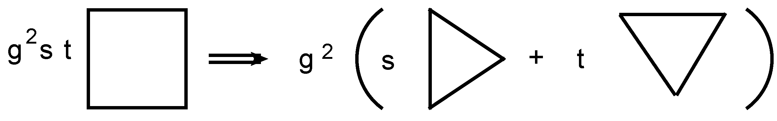
At the tree level can be found explicitly from a comparison with the expression for the four-gluon amplitude [20] obtained with the help of the six dimensional version of the BCFW recurrence relation or direct Feynman diagram computation [12,13]. This gives us that in fact has a very simple form: . Here, s and t are the standard Mandelstam variables defined as and . We also drop overall coupling constant dependence. Thus, one can see that at the tree level the four-point superamplitude can be written as:
Here, and are given by Equation (24). Note that already at the tree level the five-point amplitude is not so simple [12,13] compared to the four-point case. However, the iterated two particle cuts, which utilize only the tree level four-point amplitude, are enough to reconstruct the loop integrands up to three loops. The form of the integrand coincides with the case up to the tree level amplitude. One can argue [9,10,11] that this property will hold beyond the three-loop level.
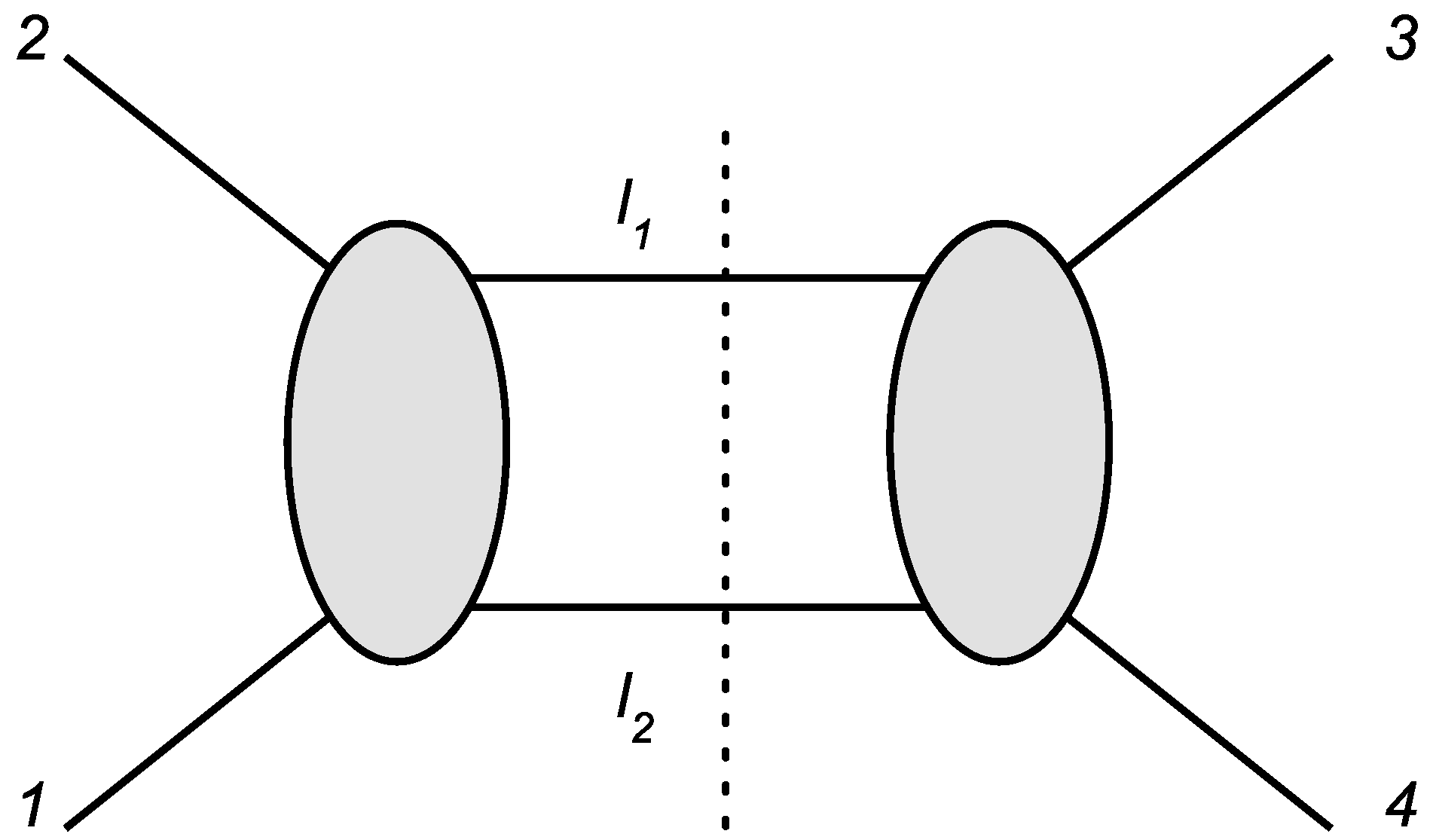
To illustrate how the unitarity cuts work, we consider a simple one loop computation(see Figure 1).
The integrand for the s-channel two particle cut of the one loop amplitude takes the form (here we explicitly label the (super)momentum dependence of the amplitudes) [20]
The integrals with respect to the Grassmannian variables can be evaluated, and after taking into account momentum conservation conditions, one gets: (the common factor is omitted)
The following formula for the Grassmannian integration is useful: ()
Equation (33) is consistent with the following ansatz for part of the amplitude associated with the s-channel cut
where is the scalar box function. The t-channel cut gives the same result, thus we conclude that the full one loop level amplitude has the form:
where is a one loop box scalar integral (see Figure 2).
Let us now consider the case. It can be constructed along the same lines as the one but in a more straightforward manner. Here, we follow [8]. The on-shell superspace can be parameterized by the following set of coordinates:
where are the Grassmannian coordinates, A and are the indices and a is the little group index. The R-symmetry group here is and carries the charge with respect to . This superspace is chiral.
The commutation relations for the supercharges in this case have the form
The supercharges in the on-shell momentum superspace representation for the n-particle state are given by
The creation/annihilation operator for the on-shell supermultiplet are
which corresponds to the physical polarizations of the gluon , two fermions , and two scalars , . Using on-shell momentum superspace Grassmann coordinates, one can straightforwardly combine the creation/annihilation operator into one “superstate” similar to the case
Here, is the absolutely antisymmetric tensor associated with the little group . No additional complications are needed.
Using the arguments identical to the previous discussion, we conclude that the color ordered superamplitude should have the form:
where is a polynomial with respect to and of degree , and the Grassmannian delta function is defined in this case as:
Here, is the absolutely antisymmetric tensor associated with the .
For the four-point amplitude, the degree of the Grassmannian polynomial is again , so as in the previous cases is a function of Bosonic variables and one can again write the four-point amplitude in the form
At the tree level can be found from a comparison with the explicit result of Feynman diagram computation or from the expression obtained as a field theory limit of the superstring scattering amplitude [8]. Similar to the previous discussion, one again has , so that at the tree level the four-point superamplitude can again be written as:
Using the iterated two particle cuts, this allows one to reconstruct the answer for the four-point amplitude up to three loops. To perform this computation, the following formula for the Grassmannian integration is useful:
Again, the form of the integrand coincides with the case (see Figure 2).
Let us now briefly discuss the situation in dimensions. The SYM supermultiplet of the on-shell states consists of the physical polarizations of the gluon and fermion fields. In this case, one encounters the following difficulty in the attempt to construct the corresponding on-shell momentum superspace: there are too many variables [12,13] to combine all the on-shell states in a manifestly Lorentz invariant manner. We need 4 variables to accommodate all the on-shell states in the theory, but the smallest representation of the little group gives 8 ’s. This problem, most likely, can be solved by using a modification of the harmonic superspace approach [21], although the resulting structure of the tree level amplitude looks complicated and no unitarity based computations have been performed thus far in such a setup.
3. The Structure of UV Divergences in the Leading, Subleading, etc. Orders of PT in SYM Theories
To calculate the amplitude, it is convenient first to extract the color ordered partial amplitude by executing the color decomposition [9,10,11]
The color ordered amplitude is evaluated in the limit , and is fixed, which corresponds to the planar diagrams. In the case of the four-point amplitudes, the color decomposition is performed as follows:
where denote the trace combinations of generators in the fundamental representation
The four-point tree-level amplitude is always factorized which is obvious within the superspace formalism. Hence, the color decomposed L-loop amplitude can be represented as
or using the standard Mandelstam variables
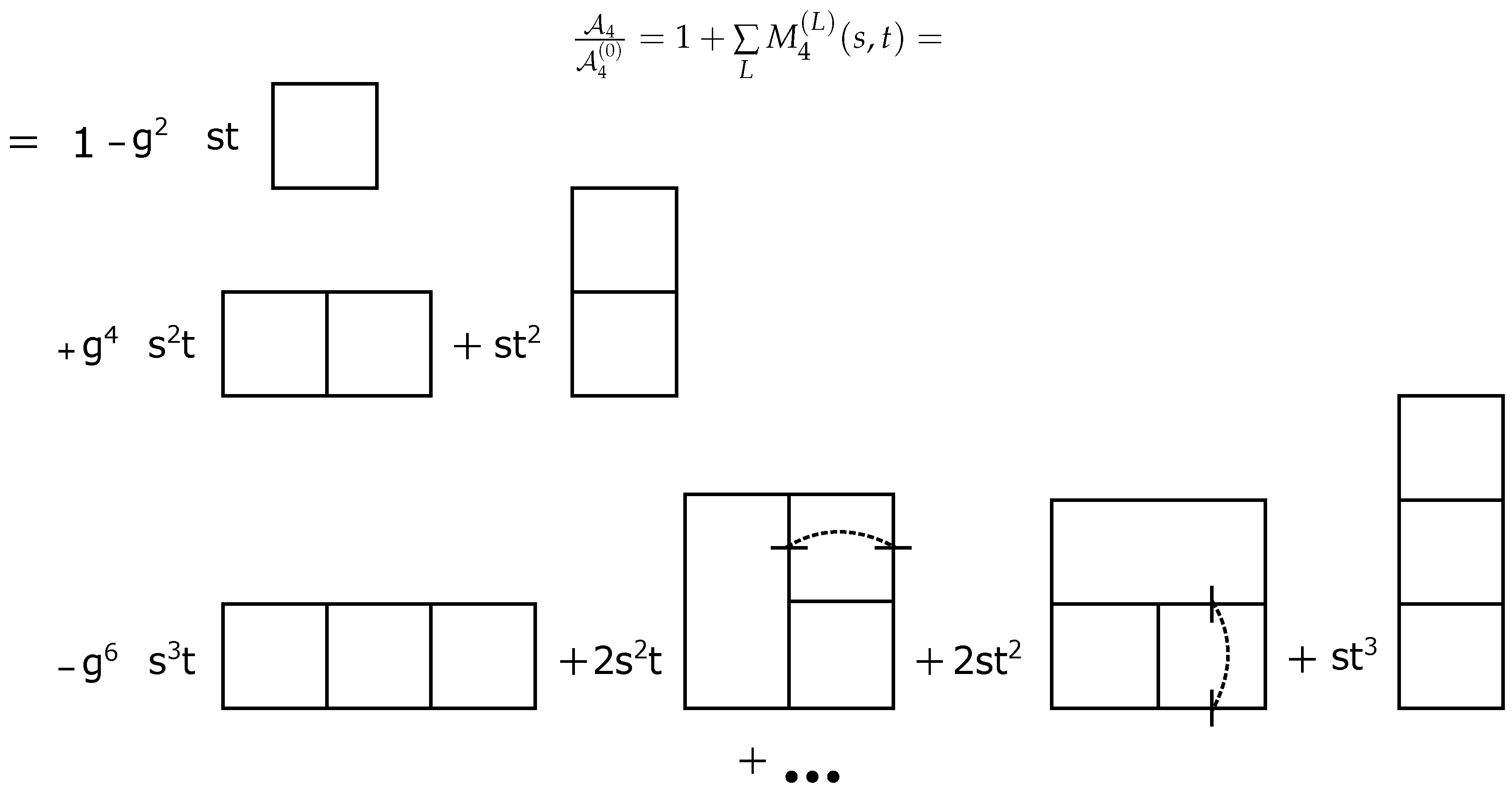
The factorized amplitude is the subject of calculation in this paper. Remarkably, it can be expressed in terms of some combination (which is universal for dimensions) of the pure scalar master integrals times some polynomial in the Mandelstam variables shown in Figure 2 [23,24].
Dimensional regularization (dimensional reduction) is common for calculation of UV divergences since the latter is manifested as pole terms with the numerators being the polynomials over the kinematic variables. In D-dimensions, the first UV divergences start from L = 6/(D-4) loops; therefore, in D = 8 and D = 10 SYM theories, they start already at one loop. As one can see in Figure 2, all the bubble subgraphs as well as triangles are entirely omitted in PT of any order, which is the result of maximal supersymmetry, and appear only in less symmetric cases. In the D = 4 and N = 4 case, this means the abandonment of all the UV divergences since the boxes are finite whereas at higher dimensions they are non-renormalizable by power counting.
In general, has the form
where , the are some monomials of s and t, and the is one of the master integrals in D-dimensional Minkowski space shown in Figure 2. The complete list of the master integrals up to five loops is presented in [23,24].These master integrals are universal for any dimension.
We use the following definition of the L-loop master integrals applied throughout the paper
Since we are interested in the UV divergences only, there is no need to calculate the multi-loop diagram itself. The task is reduced to the extraction of the pole terms that essentially simplifies the calculation. To do this, we use the BPHZ -operation [25,26,27,28,29].
For any local quantum field theory, it is inherent that, after performing the incomplete -operation, e.g., -operation, the remaining UV divergences are always local. Due to this peculiarity, it is possible to produce the so-called recurrence relations, which link the divergent contributions in all orders of perturbation theory (PT) with the ones of the lower order. These relations are known as pole equations (within dimensional regularization) in renormalizable theories [30] and can be expressed in the form of the renormalization group. This holds true for any local theory, though can be trickier to execute technically, as we showed in [16,17]. We recall the main steps of this procedure below.
The incomplete -operation (-operation) subtracts only the subdivergences of a given graph while the full -operation is defined as
where is an operator that extracts out the singular part of the graph and - is the counter term corresponding to the graph G. Applying the -operation to a given graph G in the n-th order of PT, one gets a series of terms presented below:
where terms such as or , originate from the k-loop graph which remains after subtraction of the -loop counterterm. The resulting expression has to be local and hence does not contain terms such as from any l and k. This requirement leads to a sequence of relations for and , which can be solved in favor of the lowest order terms
It is also useful to write down the local expression for the terms (counterterms) equal to
Then, one has, respectively,
This means that, by performing the -operation of the higher order diagrams, it is possible to deal only with the one-, two-, or three-loop subgraphs surviving after contraction of subdivergences and get the desired leading pole terms via Equation (54) in the leading, subleading and sub-subleading order, respectively. The latter can be evaluated in all loops algebraically.
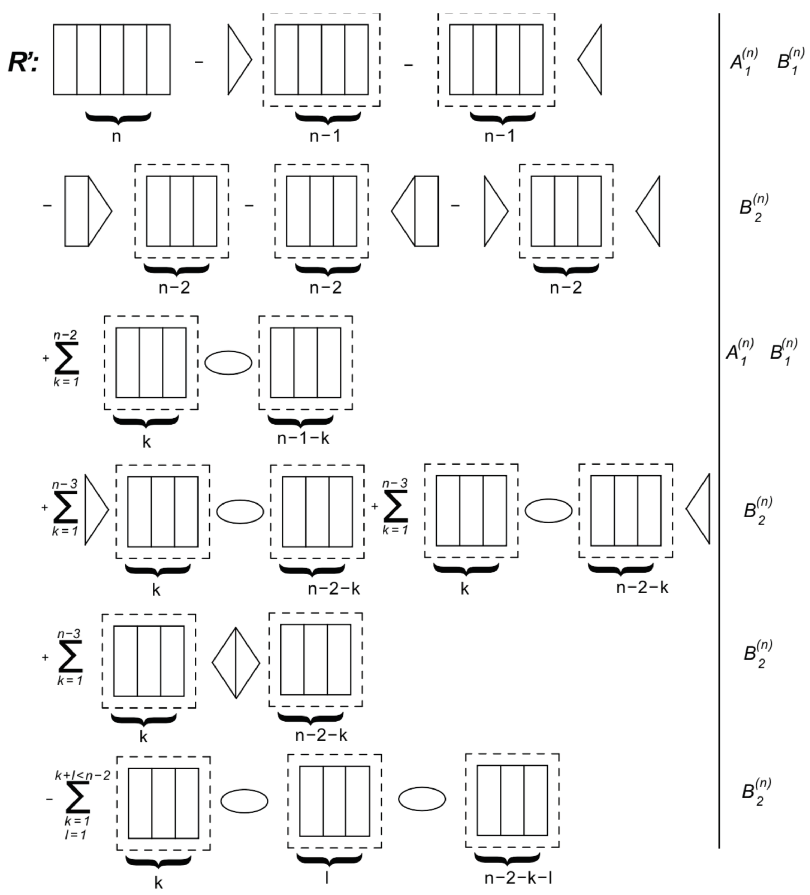
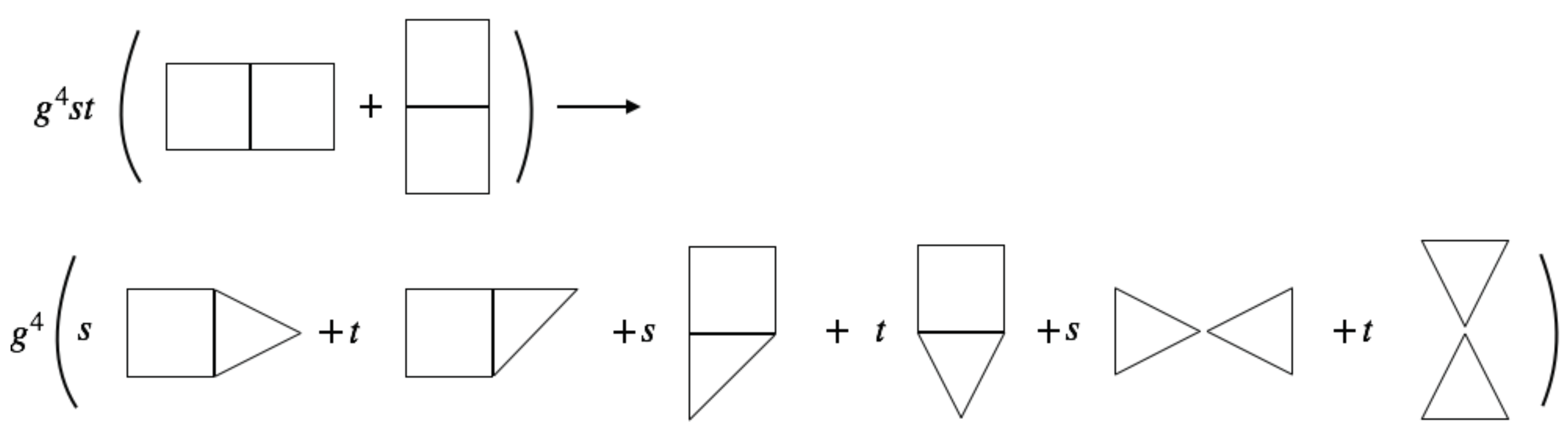
The discussed procedure makes it possible not only to derive solutions for a fixed number of loops but also to obtain the recurrence relations in any loop order. We demonstrate this derivation by the example of the horizontal ladder-type diagrams in [17] (see Figure 3).
We start with the leading order. First, one can simplify the notation and since the horizontal ladder-type diagrams in the leading order depend only on s. By calculating the one-loop diagrams shown in the first and third lines of Figure 3 and substituting them into Equation (54), we receive the recurrence relation in the leading order.
where . Starting from one-loop term, the leading divergence in any loop order can be calculated using this recurrence relation solely algebraically.
In the subleading order, one has already the t dependence but it is linear. To separate it, we use the notation and . To derive the recurrence relation in the subleading case, one has to calculate the two-loop diagrams shown in the second and last lines of Figure 3. We begin with the primed quantities since they actually enter into the recurrence relations
where , , .
Proceeding in a similar way one can get relations for the unprimed quantities. The recurrence relations for the sub-subleading divergences are not presented here due to their length.
Solving the recurrence relations in Equations (57)–(59) is complicated. However, since we actually need the sum of the series, we perform the summation multiplying both sides of Equation (57) by and take the sum from 3 to infinity. After some algebraic manipulation and introducing the notation , we finally transform the recurrence relation to the differential equation. In the leading order, we get (here )
Similar differential equations can be constructed for and ,
with
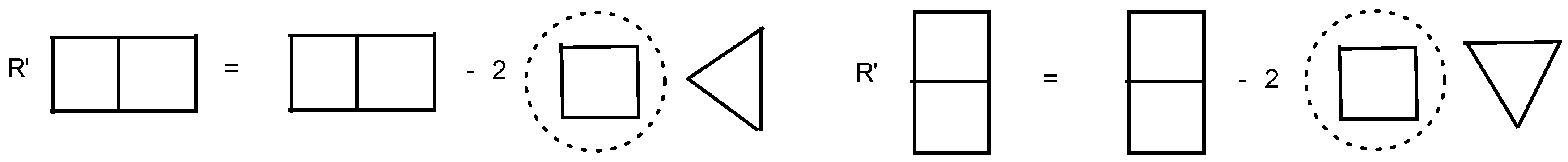
One can perform the same procedure for a specific series of diagrams as well as for the entire set by using some symmetry arguments. In [16], we constructed the full recurrence relations for the leading divergences for SYM theories in D = 6 and D = 8, 10. This was performed by consistent application of the -operation and integration over the remaining triangle and bubble diagrams with the help of Feynman parameters. While executing this, we notice that the full set of UV divergent diagrams (master integrals) consists of the s-channel and t-channel ones, and it is needed simply to add the box to the corresponding channel in order to move from to n loops. Denoting by and the sum of all contributions in the nth order of PT in s and t channels, respectively, so that
we get the following recursive relations for the and cases, respectively:
where , , and .
where .
where . The leading divergences in any order of PT can be designed in algebraic form using these recurrence relations, starting from the known values of and .
Similar to the ladder case, these recurrence relations include all the diagrams of a given order of PT and allow summing all orders of PT. This can be done by multiplying both sides of Equations (64)–(66) by , where and summing up from to infinity. Denoting the sum by , we finally obtain the following differential equations in the and cases:
The same equations with the replacement are valid for .
4. Properties of the Solutions and Numerical Analysis
Since Equations (67)–(70) are integro-differential, their analytical solution is problematic. Therefore, we use the ladder type diagrams, which are much simpler and allow for the explicit solution, as an approximation to the solution of the exact equations. We show that the ladder type diagrams are in good agreement with the total PT series and may serve as a model for the full answer.
4.1. The Ladder Case
4.1.1. D = 6
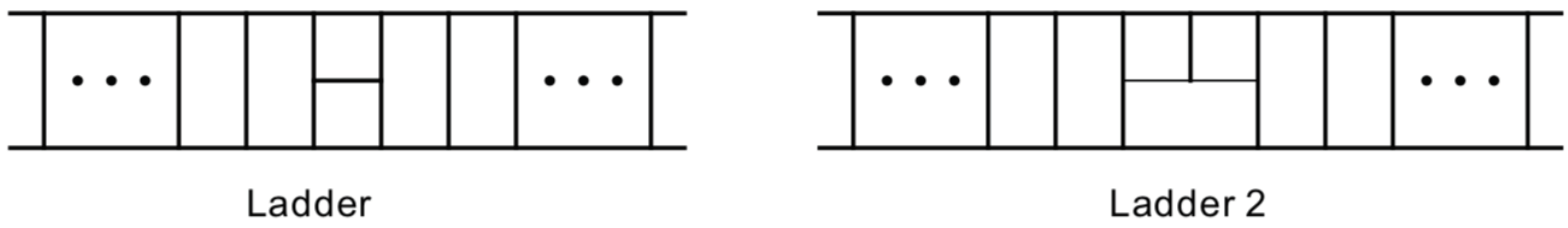
The D=6 case is of particular interest since the boxes are finite. Therefore, the s-ladder type diagram of interest contains one tennis-court subdiagram and the ladder added from the left or right (see Figure 4, left).
Using the recursive relations (see [16]), one can obtain the equation for the ladder diagrams; however, it is also possible to derive it from Equation (67). These diagrams contain only s-dependence, so it drops out from the integrals in the right-hand side of Equation (67) for the first term. The second term corresponds to the t-ladder subdiagrams and does not give a contribution to the ladder approximation. As a result, we have the ordinary differential equation
Here, is dimensionless and depends on a single dimensionless argument .
Solution to this equation is
For the vertical ladder, we have the same solution with the replacement .
Depending on the sign of s, the obtained solution tends either to infinity or to a constant when . We show further that the full solution has the same behavior and discuss its consequences below.
One can derive a similar equation for the next sequence of ladder type diagrams, which starts from four loops (Figure 4 right). The resulting expression also contains only s-dependence except for one power of t. This leads to two coupled recursive relations and hence two coupled differential equations. The solution of these equations has the form
4.1.2. D = 8
In this case, the ladder starts already from one loop. It also contains only s-dependence, so all the integrals in Equation (68) are trivial for the first terms in the bracket while the second terms have no contributions to the s-ladder like in the previous case. Then, Equation (68) reduces to the ordinary nonlinear differential equation
Here, is also dimensionless and depends on the single dimensionless argument .
This equation refers to Riccati type equations with constant coefficients. The solution has the form
This function has an infinite number of periodical poles and there is no simple limit when regardless of kinematics. Further, we show that this property also characterizes the full solution.
4.1.3. D = 10
This case looks similar to D = 8 but becomes more complicated due to the genuine box diagram in D = 10. Contrary to D = 8, this diagram is not a constant but is proportional to . Consequently, the s-ladder has dimension and consists of two parts, one proportional to s and the other to t times dimensionless function of
Equation (70) reduces to the ordinary nonlinear differential equation as in the D = 8 case; however, we have two coupled equations for and . To obtain these equations in a simple way, one needs to use the recursive relations [16]
Note that both functions are dimensionless and depend on the single dimensionless argument .
The solution of the first equation is
while the second one is expressed in the form
where the function is the solution to the nonlinear differential equation
This is also a dimensionless function of the single dimensionless variable . The solution of Equation (79) is
The behavior of is similar to in the D = 8, i.e., it possesses an infinite number of periodical poles. There is also a single pole in the function for positive values of s.
4.2. The General Case
In this subsection, we analyze Equations (67), (68) and (70) that give us the sum of infinite series of diagrams. Due to complexity of these equations, a numerical solution can be a suitable method, although this approach also has its difficulties. We cannot use the standard recursive algorithm because unknown functions are under the integral and depend on integration variables in a complex way.
We use an algorithm that is a combination of the standard numerical method and the method of successive approximations. First, we select some initial value of the function and then start with it. If we start with , then a suitable choice is . After that, we substitute it in the right-hand side and perform formal integration to get the following approximation for :
which is now a polynomial over s and t. At this step, the right-hand side is calculated with equal to a constant.
The next step is setting up of the polynomial in the right-hand side. Changing the arguments and , we perform the integration. This generates the next approximation value of : . Continuing this procedure, we generate the highest degree polynomials s and t at each step. However, starting with 3–4 iterations, the length of the polynomials becomes too time consuming for further calculation. At this step, we estimate the value of with the fixed values of s and t, for example, s = t = 1. The calculated value gives us a constant, which we identify with the value of at . We use this value to run the same procedure again for the next iteration. This way, we calculate the values of at the points along the axis .
Then, we interpolate all obtained points to a smooth function. We found that makes the solutions stable. The numerical results demonstrate a reasonable approximation being applied to the known functions, although this method is not justified.
Note that, after calculating the function , we can replace its argument having in mind that it depends on the dimensionless combinations and (and the same for t) for 6, 8 and 10, respectively, for dimensional reasons.
It should also be said that, in the 8 and 10 cases, the form of Equations (68) and (70) is not suitable for numerical analysis since the second term contains an infinite sum with an infinite number of derivatives. Cutting this sum makes the numerical solution unstable. To avoid this problem, we note that the construction resembles an ordinary shift operator with slightly modified coefficients. This infinite sum can be removed by introducing two additional integrations, which do not cause difficulties in numerical integration. One has:
We use this technique for numerical calculations in the case of and . The results of application of the described techniques for all three cases are presented below.
To test our numerical procedure, we compared the results of our calculation with the results obtained using PT, the Pade approximation and the Ladder approximation. For comparison, we used the first 15 terms of the PT series that are generated using our recurrence relations. This seemed to be far enough since the successive PT coefficients are falling rapidly.
The next step is to use the Pade approximation. This is not always stable since Pade approximations sometimes have fictitious poles. It is a well-known feature, and we tried to avoid it using mainly diagonal approximations. With 15 terms of PT, the (6,6), (6,7) and (7,7) approximants are almost identical and give a smooth function.
The third curve in the graphs corresponds to the ladder approximation. Analytical solutions here are given by Equations (71), (74), (77) and (80) from the previous subsection. In the case of D = 6, we also considered the second ladder, which is based on the tennis court diagram in the t-channel (see Figure 4) and is given by Equation (72).
Finally, we built a numerical solution obtained by the iteration procedure described above. In the case when the function has poles, we built a numerical solution separately for each finite interval.
The function is a function of three variables. However, as mentioned above, for dimensional reasons, it has only two independent dimensionless arguments. In 6, 8 and 10, they are , and , respectively. We constructed both two-dimensional graphs with and three-dimensional graphs in the plane for better presentation.
4.2.1. D = 6
In D=6, the PT series looks like
where the dots stand for the higher order terms. We used 15 terms for numerical comparison with the other approaches.
From Equation (82), we constructed the diagonal Pade approximant [7/7] as a function of a new variable in the case when . It has the form
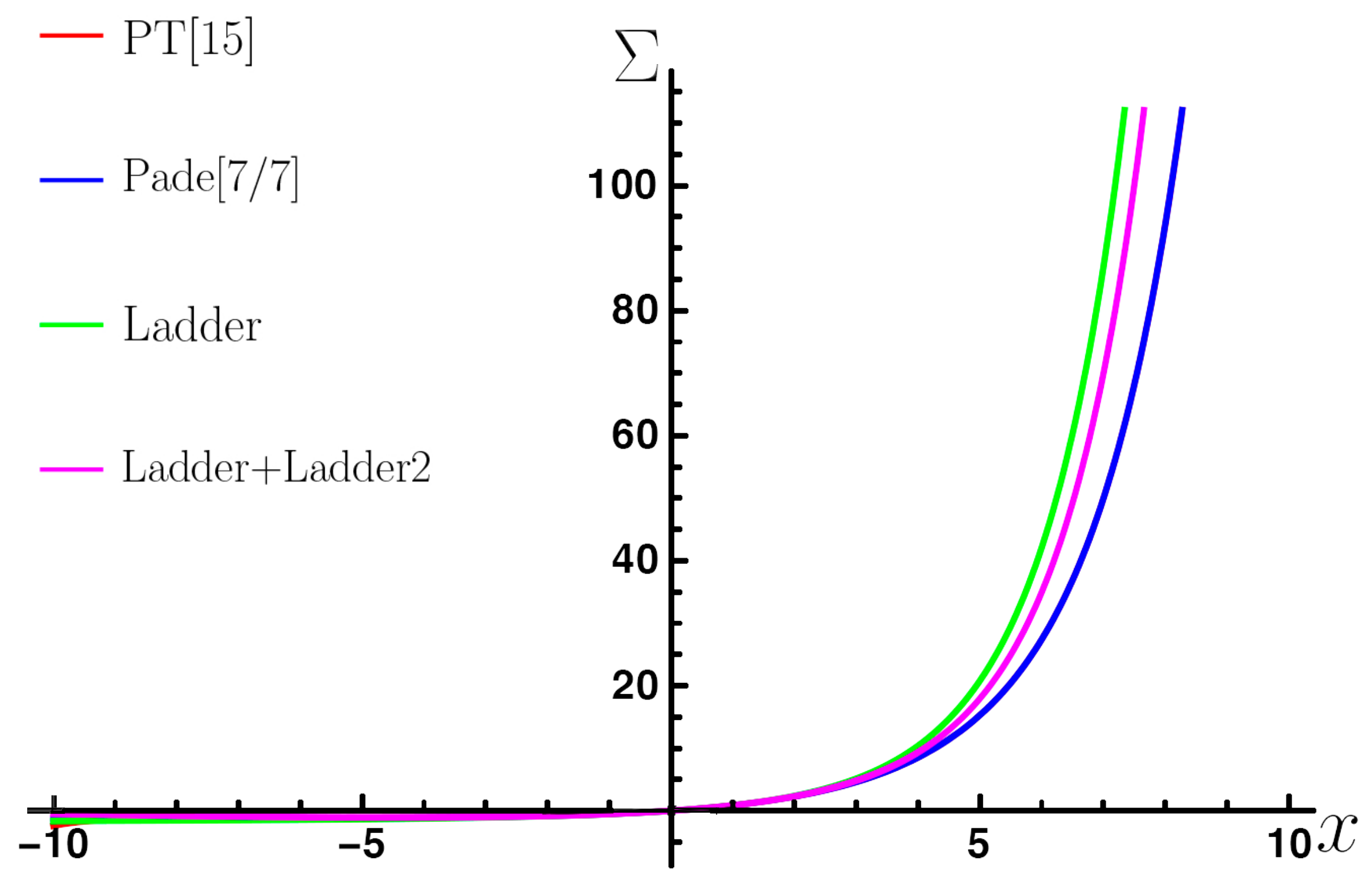
The ladder approximation is given by Equation (71) and the second ladder by Equation (72) with . The numerical solution starts from and in this case has only one interval. To demonstrate the behavior of the function obtained by different approaches and compare them all together, we built two types of graphs. The first one, shown in Figure 5, contains four different curves corresponding to four different approaches.
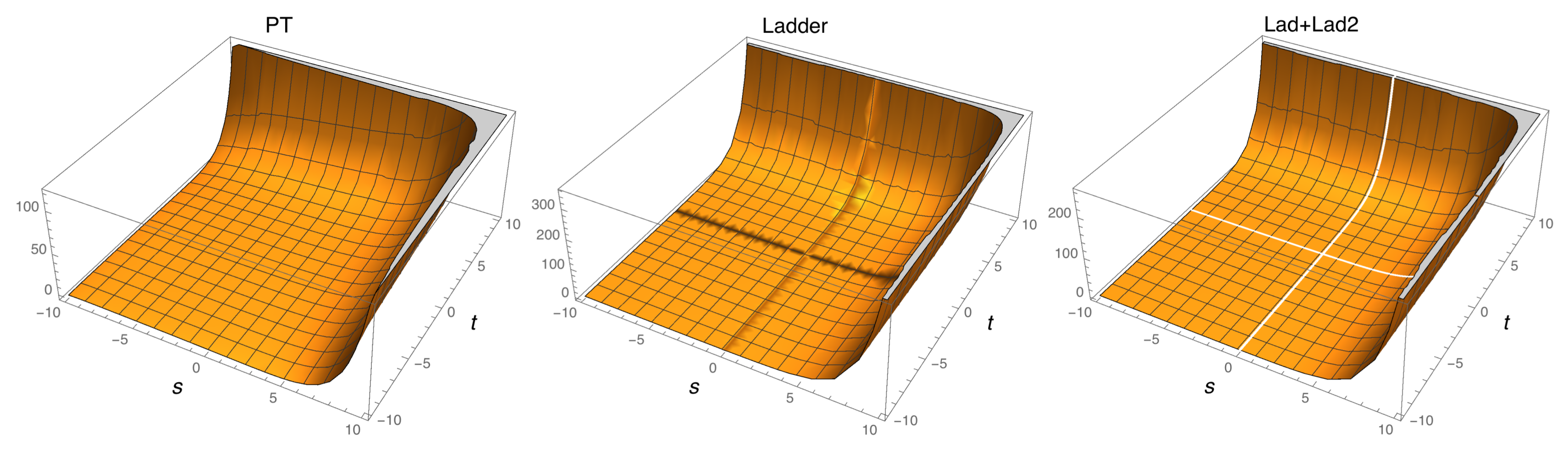
The second graph is a three-dimensional plot shown in Figure 6. Here, we plot the PT approximation, the ladder approximation and the second ladder approximation.
The first graph shows that all curves have almost the same behavior. Analytically, it is perfectly described by a ladder approximation. This is also confirmed by the three-dimensional graph shown in Figure 6. The inclusion of the second ladder does not change the solution qualitatively but provides a better match with PT. The function has no restrictions for () for and tends to a fixed point when . This limit would correspond to the removal of the UV regularization. It can be seen that the summation of the entire infinite series does not lead to a finite theory.
4.2.2. D = 8
In the case of D = 8, the PT series starts already from one loop and has the form
For , the [7/6] Pade approximant is
where now .
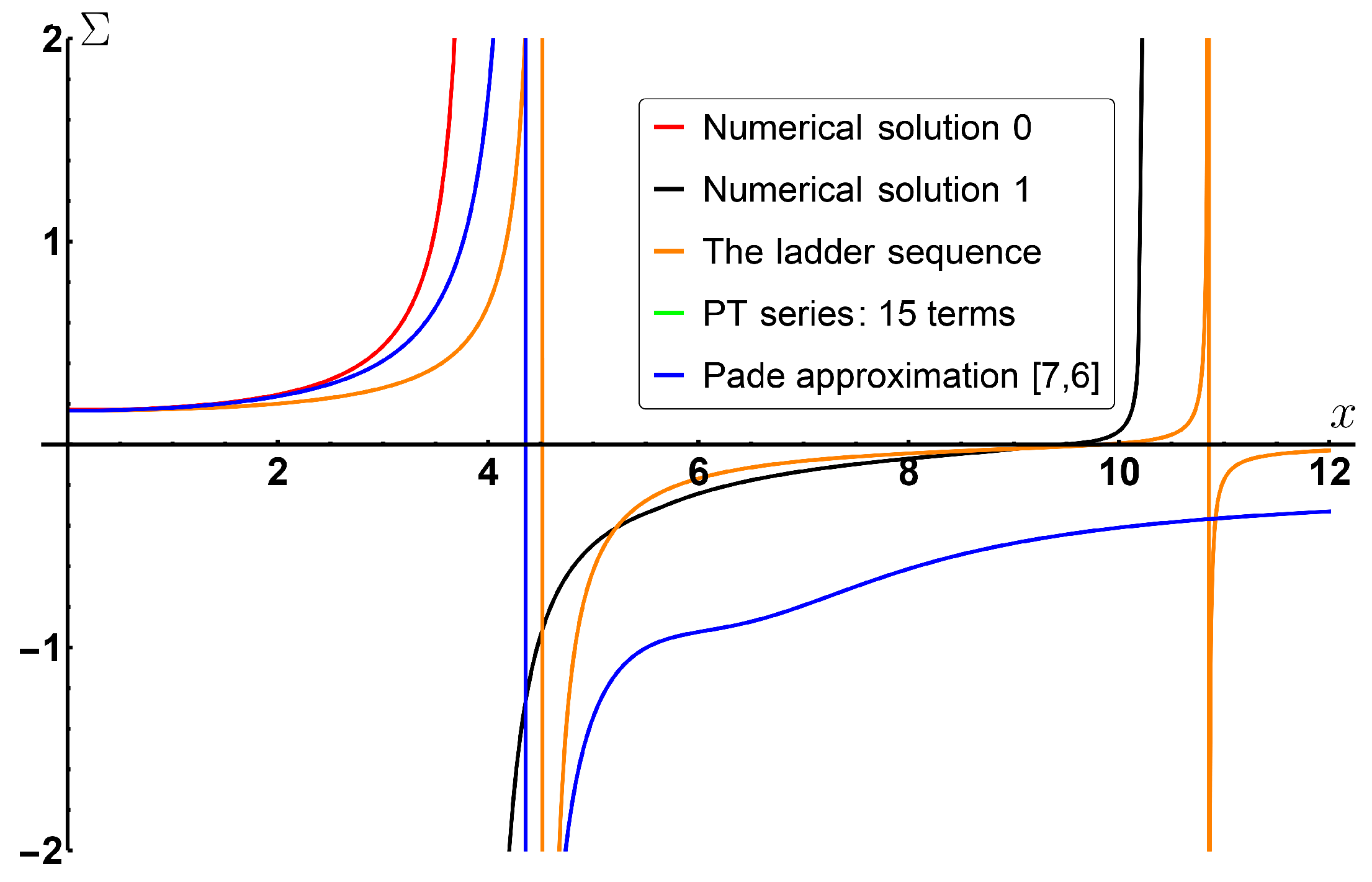
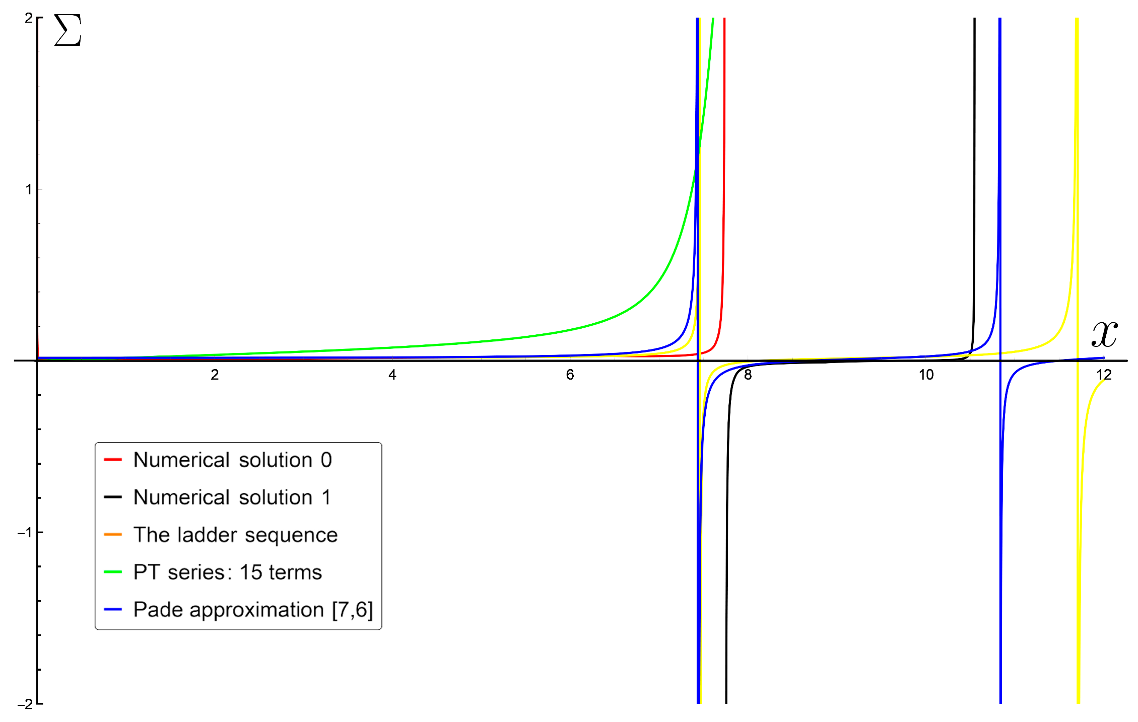
The ladder approximation is given by Equation (74). The numerical solution starts with and continues to the first pole . Then, we start it again for and reach the second pole at and so on. The poles coincide with the poles in the ladder approximation (Equation (74)). A comparison of various curves for is shown in Figure 7.
It can be seen that in the first interval all curves almost coincide. The PT curve exists only in the interval below the first pole. The Pade curve reproduces the first pole but does not fit to the others. The numerical curve reproduces both poles and is close to the ladder approximation.
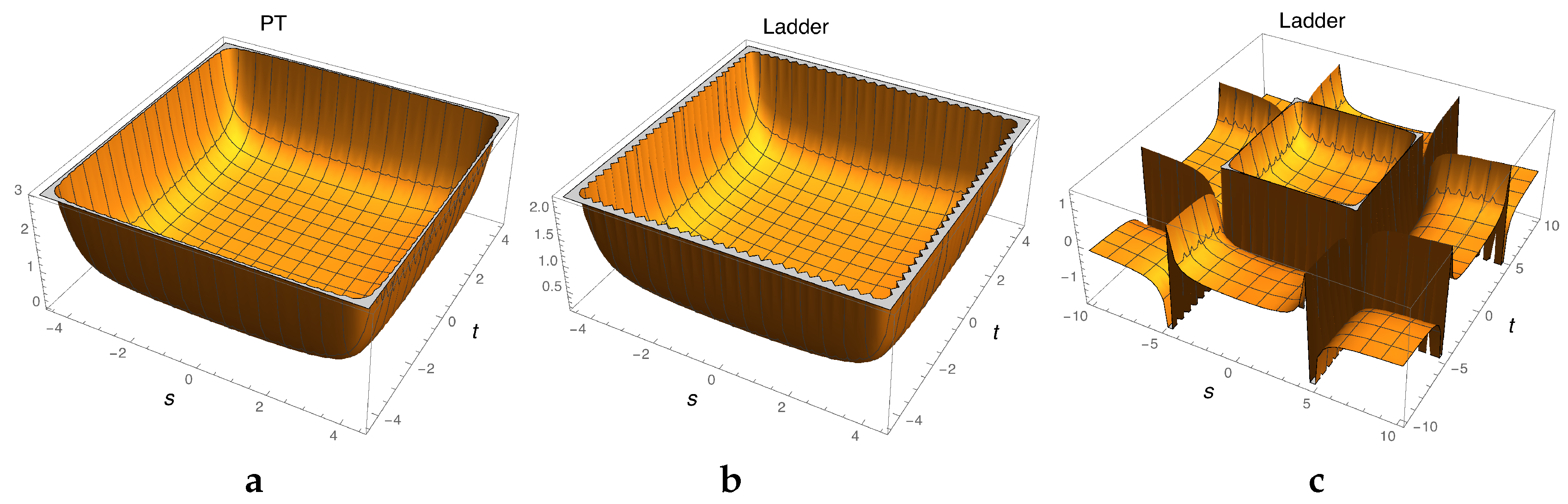
We present also the three-dimensional plot in the plane for in Figure 8.
It can be seen that the ladder as in the case of gives a very accurate approximation to PT and allows you to go beyond the limits of the first pole. A comparison of the ladder approximation and the numerical solution of the complete equation confirms our conclusion that the ladder approximation gives the correct behavior of the function.
Again, we must admit that the limit () does not exist. The function has an infinite number of periodic poles for any choice of kinematics. Therefore, finiteness is not achieved when the sum over the entire cycles is taken into account.
4.2.3. D = 10
This case is quite similar to the one. The PT series is now
while the [6/7] Pade approximation for reads
where .
The ladder approximation is given by Equations (77) and (80), and the numerical approximation is constructed first for the interval from to the first pole, then continues to the second, etc. The comparison of all the curves is shown in Figure 9.
The situation here is the same as in the case of . The ladder approximation works quite well, and its analytical solution qualitatively describes all the features of the full equation. The function obeys an infinite number of periodic poles and one single pole is obtained from (Equation (80)). There is no limit when .
Since the removal of the regularization () does not lead to finite amplitudes, it is necessary to perform a kind of renormalization procedure. It has some peculiarities because these theories are nonrenormalizable.
5. The Renormalization Procedure
All higher dimensional gauge theories are non-renormalizable. Of course, the scattering amplitudes can be made finite by subtracting all UV divergences in some way. This is not a problem. The problem is that the counter terms do not repeat the original Lagrangian and one gets new structures with increasing power of momenta at each step of perturbation theory. This means that, subtracting the UV divergence each time, one has to define the normalization of a new operator, thus having a new arbitrary constant. The number of these constants is infinite. However, as we demonstrate above, all the higher order divergences are related via the generalized RG equations. Hence, changing the subtraction condition at a given loop, one consistently changes the normalization condition of an infinite set of operators. Hence, one may hope to relate them removing the arbitrariness.
5.1. The Scheme Dependence
All our considerations thus far are based on the minimal subtraction scheme. To trace what happens when one changes the normalization condition, we consider now the non-minimal subtraction scheme. As an example, we take the case where divergences appear already in one loop.
Obviously, the leading divergences are scheme independent but the subleading ones depend on a scheme. However, this dependence in all orders of PT is defined by a single arbitrary constant which appears in subtraction of a single one-loop box-type diagram. The recurrence relations obtained above are scheme independent. Indeed, if one chooses the one-loop counter term in the form
( corresponds to the minimal subtraction scheme), then using the recurrence relations for the subleading divergences, one gets the following additional term to the sum of the counter terms in all orders of PT (remind the notation )
Thus, the arbitrariness in the counter terms with an infinite number of derivatives is reduced in the leading order to the choice of the single parameter . It is equivalent to a finite change of the renormalization constant
This is exactly what happens to renormalizable interactions except that there we redefine a single coupling and here it is an infinite series of couplings with increasing power of derivatives.
Consider now what happens in the sub-subleading order. In this case, the dependence on the subtraction scheme is contained also in the two-loop box-type diagram. Following the subleading case, we choose the counter term in the form
where comes from the one-loop counter term and is the new subtraction constant. Using the recurrence relation for the sub-subleading divergences, one gets the following additional term proportional to in all orders of PT:
This corresponds to the finite renormalizations
This simple pattern obviously has a one-loop origin since it comes from the leading divergences and they are defined by the one-loop box diagram.
The situation with dependence on in the sub-subleading order is more complicated. There are two contributions here: the linear and quadratic. The quadratic dependence obviously appears from the substitution of Equation (90) into the minimal scheme counter term (Equation (89)), which gives the second derivative of . However, the redefinition of the coupling contains an extra part compared to Equation (93), which is proportional to that gives the first derivative of . All together, the full quadratic dependence has the form
Using the recurrence relations in the sub-subleading order, we have checked that this result is valid in all orders of PT.
The situation with the linear term is not that straightforward. It is not given by the leading term only but involves also the subleading one. Here, for the first time, we meet the situation where the renormalization is not reduced to a simple multiplication. It happens because the subleading terms depend on both s and t and one cannot separate them anymore.
This is clearly seen in the third order of PT. Namely, if we consider the -operation of the three-loop box diagram and calculate the arbitrariness , which is due to arbitrariness in the two-loop counter-term (the last diagram in Figure 10).
The latter is independent of the t contribution. The reason is that, while the two loop box contains the t contribution in the subleading order, the arbitrariness is contained only in the s term. At the same time, when one evaluates the sub-subleading divergence in the three-loop box diagram using the -operation, one has a nonzero contribution from both the s and t terms in the last diagram in Figure 10. The two expressions are obviously unrelated
whereas in three loops has the following form:
The discrepancy comes from this last term in Figure 10. To see this, we subtract the unmatched t contribution from and compare it with . We call it
Taking the derivative with respect to z, one reproduces the desired result
The situation repeats itself in the fourth order of PT being even more tricky.
This consideration shows us what actually goes wrong in the renormalization procedure and suggests the right way to formulate it. The key reason is that the divergent expressions and, hence, the counter terms are not constants anymore but are polynomials of momenta. This means that this momentum dependent counter terms have to enter inside the integrals when performing the -operation, i.e., this is not a simple multiplication procedure anymore.
5.2. Kinematically Dependent Renormalization
Based on the performed analysis, below we describe how the renormalization procedure can be reformulated in non-renormalizable theories and illustrate it by the example of two- and three-loop divergences in D = 8 SYM theory. Formally, it looks precisely like a familiar renormalization procedure in any renormalizable theory, but the renormalization constant Z becomes the function of kinematic variables and acts on the amplitude not as a simple multiplication but as the operator in momentum space. Namely, to remove all the UV divergences in the amplitudes and get a finite answer, one follows the usual prescription multiplying the bare amplitude by the proper renormalization constant and replacing the bare coupling with the renormalized one:
where is the ratio (). Remember also that the renormalization constant can be calculated diagrammatically with the help of the following standard operation [31]:
The essential difference between the non-renormalizable and the renormalizable cases manifests itself in momentum dependence of the renormalization constant Z. This actually means that it becomes the operator acting on the amplitude according to the rules of the -operation. To demonstrate how this renormalization procedure works, we apply Equations (99) and (100) to the singular part of the amplitude
order by order in PT.
In the one-loop order, the coupling is not changed and the renormalization constant is chosen in the form . This leads to a finite answer. Notice that the renormalization constant is not really a constant but depends on the kinematic factors s and t!
In the two-loop order, the coupling is changed now according to Equation (100), namely,
and the renormalization constant is taken in the form
where the coefficients and have to be chosen in a way to cancel all divergences both local and nonlocal ones.
Consider how it works in practice: When substituting Equations (103) and (104) into Equation (99), one can notice that the replacement of by Equation (103) in the one loop term (∼) and multiplication of one loop contributions from the renormalization constant and from the amplitude have the effect of subtraction of subdivergences in the two loop graph. This is exactly what guarantees the locality of the counter terms within the -operation. However, contrary to the renormalizable case, here the renormalization constant contains the kinematic factors, the powers of momenta, which are external momenta for the subgraph but are internal ones for the whole diagram. This means that, evaluating the counter term, they have to be inserted inside the remaining diagram and integrated out. To clarify this point, we consider the corresponding term which appears when multiplying the one loop Z factor by the one loop amplitude. The s and t factors from the Z factor have to be inserted inside the box diagram, as shown in Figure 11.
This means that the usual multiplication procedure has to be modified: the Z factor becomes the operator acting on the diagram which inserts the powers of momenta inside the diagram. This looks a bit artificial but exactly reproduces the -operation for the two loop diagram shown below in Figure 12.
One can see that the one-loop divergences (∼) cancel and the cancellation of the two-loop ones requires
One deduces that , thus the renormalization constant takes the form
which exactly corresponds to the one obtained using Equation (101). This expression now has to be substituted into Equation (100) to obtain the renormalized coupling. Note that it also depends on kinematics.
The same way, one can trace the action of the Z-operator in the three-loop diagram, as shown in Figure 13. In this case, besides the three-loop box diagram, one also has the tennis-court one, and the resulting counter terms correspond to both of them.
In the context of the present discussion, the transition to a non-minimal scheme is equivalent to the multiplication of the amplitude by the finite renormalization constant
and the corresponding finite change of the coupling g. This looks similar to the renormalizable case though the meaning is different. Again, not only the multiplication but also the action of the operator is kinematically dependent. Therefore, it is not a simple change of a single coupling but of the whole infinite series of higher derivative terms. Similarly, the subtraction arbitrariness of the double box influences the sub-subleading divergences and results in higher order terms in Equation (108) as in Equation (107), just as in renormalizable theories [18]. Therefore, the whole arbitrariness is accumulated in one renormalization constant evaluated order by order in PT, which acts as an operator and generates an infinite series of terms. In fact, this means that we build this way an induced higher derivative theory where higher terms appear order by order of PT with fixed coefficients. For instance, the one-loop term generates the gauge invariant counter term
that contains higher derivatives as well as new vertices with extra gauge fields, etc.
6. High Energy Behavior
Assuming that one accepts these arguments, there is still a problem that at each order of PT the amplitude increases with energy, thus violating the unitarity. However, apparently, this problem has to be addressed after summation of the whole PT series. While each term of PT behaves badly, the whole sum might behave differently.
To analyze the high energy behavior of the full amplitude, one can use the solutions of the generalized RG equations obtained above. Indeed, as in any renormalizable case, the high energy behavior is associated with the UV divergences. Considering the case when and expanding the amplitude over , one finds the one-to-one correspondence between the coefficient of the leading pole and the leading asymptotic term : Thus, , as considered in Section 4, corresponds to the limit .
Having this in mind, we can analyze the high energy asymptotics of the amplitudes in and 10. The task becomes more complicated since we have the function of two variables and one may have different limits in different directions. We looked for the case when and corresponding to the center of mass frame.
In the D = 6 case, in the leading order, the full amplitude behaves qualitatively similar to the ladder. For the partial amplitude, it contains the exponent , and, since , one has a decreasing exponent and hence a smooth function of energy without violation of unitarity. The same is true for the partial amplitude. However, for the amplitude, one has , which results in increasing exponent. This amplitude obviously violates unitarity and spoils the picture. The subleading asymptotics does not improve the situation having the same type of behavior.
In the D = 8 and 10 cases, again, the ladder diagrams qualitatively correctly reproduce the behavior of the full amplitude. Here, all partial amplitudes behave similarly. They have poles for finite values of z and, hence, for finite values of E. This is similar to QED; however, in this case, the pole is much closer due to the power law behavior of the function. There are multiple poles. Thus, again, one has problems with unitarity at high energy.
It would be interesting to find an example of a theory where such kind of summation leads to a smooth high energy limit such as in asymptotically free theory in the renormalizable case.
7. Discussion
Our main concern here was the understanding of the structure of UV divergences in supersymmetric gauge theories with maximal supersymmetry.
We restricted ourselves to the on-shell scattering amplitudes, since after all it is the S-matrix, which we want to make finite.
Our main results can be formulated as follows:
- (1)
- The on-shell scattering amplitudes contain the UV divergences that start from one loop (three loops) and do not cancel (except for the all-loop cancellation of the bubbles and triangles).
- (2)
- These divergences possess increasing powers of momenta (derivatives) with increasing order of PT. For the four-point scattering amplitude, this manifests itself as increasing power of the Mandelstam variables s or t. This means that the theory is not renormalizable by power counting.
- (3)
- Nevertheless, all the higher loop divergences are related to the lower ones via explicit pole equations which are the generalization of the RG equations to the case of non-renormalizable theories. The leading divergences are governed by the one-loop counter term, the subleading ones by the two-loop counter term, etc. This happens exactly as in the well known case of renormalizable interactions.
- (4)
- The summation of the leading and subleading divergences can be performed by solving the generalized RG equations. The solution to these equations depends on dimension and has a different form in different dimensions. For particular sets of diagrams, one can get an analytical solution, while in the general case it is only numerical.
- (5)
- In D = 6, the solution is characterized by the exponential function that decreases for some partial amplitudes and increases for the other as a function of . In D = 8 and D = 10, the solutions possess an infinite number of poles. This means that they do not have a finite limit when () which would correspond to the finite answer when removing the regularization.
- (6)
- We reformulate the multiplicative renormalization procedure with replacement of the renormalization constant by an operator that depends on kinematics. As a result, one can construct a higher derivative theory that gives finite scattering amplitudes with a single arbitrary coupling g defined in PT within a given renormalization scheme. Transition to another scheme is performed by the action on the amplitude of the finite renormalization operator.
- (7)
- The high energy behavior of the amplitudes is governed by the generalized RG equations just as in renormalizable theories. In the three examples that we considered, this behavior is different but in all cases the amplitudes either increase with energy or hit the pole at finite energy, as in QED.
- (8)
- Thus, the maximal supersymmetric gauge theories at higher dimensions despite many attractive features still happened to be inconsistent at high energies. We hope that the methods of analysis developed here can be used in other non-renormalizable theories including gravity.
Author Contributions
Investigation, D.K., L.B., A.B., D.T. and D.V.; writing—original draft preparation, D.K., L.B., A.B., D.T. and D.V.; writing—review and editing, D.K., L.B., A.B., D.T. and D.V.; supervision, D.K.
Funding
This work was supported by the Russian Science Foundation grant # 16-12-10306. A. Borlakov acknowledges the support of the Russian Foundation for Basic Research, grant # 17-02-00872.
Conflicts of Interest
The authors declare no conflict of interest.
References
- Bern, Z.; Huang, Y.-T. Basics of Generalized Unitarity. J. Phys. A 2011, 44, 454003. [Google Scholar] [CrossRef]
- Elvang, H.; Huang, Y.-T. Scattering Amplitudes. arXiv, 2013; arXiv:1308.1697. [Google Scholar]
- Bartels, J.; Schomerus, V.; Sprenger, M. The Bethe roots of Regge cuts in strongly coupled N = 4 SYM theory. J. High Energy Phys. 2015, 1507, 098. [Google Scholar] [CrossRef]
- Dixon, L.J.; Drummond, J.M.; Duhr, C.; Pennington, J. The four-loop remainder function and multi-Regge behaviour at NNLLA in planar = 4 super-Yang-Mills theory. J. High Energy Phys. 2014, 1406, 166. [Google Scholar] [CrossRef]
- Bern, Z.; Carrasco, J.J.; Dixon, L.; Johansson, H.; Roiban, R. Amplitudes and Ultraviolet Behavior of N = 8 Supergravity. Fortsch. Phys. 2011, 59, 561–578. [Google Scholar] [CrossRef]
- Kallosh, R. 7(7) Symmetry and Finiteness of N = 8 Supergravity. J. High Energy Phys. 2012, 1203, 083. [Google Scholar] [CrossRef]
- Heslop, P.; Lipstein, A.E. On-shell diagrams for N = 8 supergravity amplitudes. J. High Energy Phys. 2016, 1606, 069. [Google Scholar] [CrossRef]
- Boels, R.H.; O’Connel, D. Simple superamplitudes in higher dimensions. J. High Energy Phys. 2012, 1206, 163. [Google Scholar] [CrossRef]
- Andrei Smilga, Ultraviolet divergences in non-renormalizable supersymmetric theories. Phys. Part. Nucl. Lett. 2016, 14, 245–260. [CrossRef]
- Broedel, J.; Sprenger, M. Six-point remainder function in multi-Regge-kinematics: An efficient approach in momentum space. J. High Energy Phys. 2016, 1605, 055. [Google Scholar] [CrossRef]
- Dennen, T.; Huang, Y.-T. Dual Conformal Properties of Six-Dimentional Maximal Super Yang-Mills Amplitudes. J. High Energy Phys. 2011, 1101, 140. [Google Scholar] [CrossRef]
- Caron-Huot, S.; O’Connel, D. Spinor Helicity and Dual Conformal Symmetry in Ten Dimensions. J. High Energy Phys. 2011, 1108, 014. [Google Scholar] [CrossRef]
- Cheung, C.; O’Connel, D. Amplitudes and Spinor-Helicity in Six Dimensions. J. High Energy Phys. 2014, 0907, 075. [Google Scholar] [CrossRef]
- Bork, L.V.; Kazakov, D.I.; Vlasenko, D.E. On the amplitudes in N = (1,1) D = 6 SYM. J. High Energy Phys. 2013, 1311, 065. [Google Scholar] [CrossRef]
- Bork, L.V.; Kazakov, D.I.; Vlasenko, D.E. Challenges of D = 6 N = (1,1) SYM theory. Phys. Lett. 2014, B374, 111–115. [Google Scholar] [CrossRef]
- Bork, L.V.; Kazakov, D.I.; Kompaniets, M.V.; Tolkachev, D.M.; Vlasenko, D.E. Divergences in maximal supersymmetric Yang-Mills theories in diverse dimensions. J. High Energy Phys. 2015, 1511, 059. [Google Scholar] [CrossRef]
- Kazakov, D.I.; Vlasenko, D.E. Leading and subleading UV divergences in scattering amplitudes for D = 8 SYM theory in all loops. Phys. Rev. 2017, D95, 045006. [Google Scholar] [CrossRef]
- Borlakov, A.T.; Kazakov, D.I.; Tolkachev, D.M.; Vlasenko, D.E. Summation of all-loop UV Divergences in Maximally Supersymmetric Gauge Theories. J. High Energy Phys. 2016, 1612, 154. [Google Scholar] [CrossRef]
- Kazakov, D.I. Kinematically dependent renormalization. Phys. Lett. 2018, B786, 327–331. [Google Scholar] [CrossRef]
- Dennen, T.; Huang, Y.-T.; Siegel, W. Supertwistor space for D = 6 maximal super Yang-Mills. J. High Energy Phys. 2010, 1104, 127. [Google Scholar] [CrossRef]
- Bandos, I. Spinor frame formalism for amplitudes and constrained superamplitudes of 10D SYM and 11D supergravity. J. High Energy Phys. 2018, 1811, 017. [Google Scholar] [CrossRef]
- Mafra, C.R.; Schlotterer, O. Two-loop five-point amplitudes of super Yang-Mills and supergravity in pure spinor superspace. J. High Energy Phys. 2015, 1510, 124. [Google Scholar] [CrossRef]
- Bern, Z.; Dixon, L.J.; Smirnov, V.A. Iteration of planar amplitudes in maximally supersymmetric Yang-Mills theory at three loops and beyond. Phys. Rev. D 2005, 72, 085001. [Google Scholar] [CrossRef]
- Bern, Z.; Carrasco, J.J.M.; Johansson, H.; Roiban, R. The Five-Loop Four-Point Amplitude of N = 4 super-Yang-Mills Theory. Phys. Rev. Lett. 2012, 109, 241602. [Google Scholar] [CrossRef] [PubMed]
- Bogoliubov, N.; Parasiuk, O. Über die Multiplikation der Kausalfunktionen in der Quan-Tentheorie der Felder. Acta Math. 1957, 97, 227–266. [Google Scholar] [CrossRef]
- Hepp, K. Proof of the Bogolyubov-Parasiuk theorem on renormalization. Commun. Math. Phys. 1966, 2, 301–326. [Google Scholar] [CrossRef]
- Zimmermann, W. Local field equation for A4-coupling in renormalized perturbation theory. Commun. Math. Phys. 1967, 6, 161–188. [Google Scholar] [CrossRef]
- Bogolyubov, N.N.; Shirkov, D.V. Introduction to the Theory of Quantized Fields; Nauka: Moscow, Russia, 1976; (In Russian). English Translation: Bogolyubov, N.N.; Shirkov, D.V. Introduction to the Theory of Quantized Fields, 3rd ed.; Wiley: New York, NY, USA, 1980. [Google Scholar]
- Zavyalov, O.I. Renormalized Feynman Diagrams; Nauka: Moscow, Russia, 1979; (In Russian). English Translation: Renormalized Quantum Field Theory; Kluwer: Dordrecht, The Netherlands, 1990. [Google Scholar]
- Hooft, F.T. Dimensional regularization and the renormalization group. Nucl. Phys. B 1973, 61, 455–468. [Google Scholar] [CrossRef] [Green Version]
- Vasiliev, A.N. Quantum Field Renormalization Group in Critical Behavior Theory and Stochastic Dynamics; Petersburg Institute for Nuclear Physics: St. Petersburg, Russia, 1998; English Translation: The Field Theoretic Renormalization Group in Critical Behavior Theory and Stochastic Dynamics; Chapman & Hall/CRC: Boca Raton, FL, USA, 2004. [Google Scholar]
Figure 1.
Two particle s-channel cut for the one loop SYM amplitude.

Figure 2.
The universal expansion for the four-point scattering amplitude in SYM theories in terms of master integrals. The connected strokes on the lines mean the square of the flowing momentum.
Figure 2.
The universal expansion for the four-point scattering amplitude in SYM theories in terms of master integrals. The connected strokes on the lines mean the square of the flowing momentum.

Figure 3.
The -operation for the horizontal ladder in D = 8.

Figure 4.
The ladder type diagrams in D = 6.

Figure 5.
Comparison of various approaches to solve Equation (67): PT, Pade, Ladder and Numerics. The PT and Pade curves coincide in a given interval.
Figure 5.
Comparison of various approaches to solve Equation (67): PT, Pade, Ladder and Numerics. The PT and Pade curves coincide in a given interval.

Figure 6.
Comparison of PT, Ladder and Ladder2.

Figure 7.
Comparison of various approaches to solve Equation (68). The red and black lines are the numerical solutions described in the previous section between the first pole and between the first and the second ones. The green one is the PT. The blue one is the Pade approximation. The yellow one represents the Ladder analytical solution.

Figure 8.
Comparison of PT (a) and the ladder approximation (b) in the region up to the first pole and (c) the ladder approximation beyond the first pole. One can clearly see the pole structure of the function .
Figure 8.
Comparison of PT (a) and the ladder approximation (b) in the region up to the first pole and (c) the ladder approximation beyond the first pole. One can clearly see the pole structure of the function .

Figure 9.
Comparison of various approaches to solve Equation (70). The red and black lines are the numerical solutions described in the previous section before the first pole and between the first and the second ones. The green one is the PT. The blue one is the Pade approximation. The yellow one represents the Ladder analytical solution.

Figure 10.
-operation for the three-loop box diagram.

Figure 11.
Action of the Z-operator at the two loop level.

Figure 12.
-operation for the two loop diagrams.

Figure 13.
Action of the Z-operator at the three loop level. The first, second and the last two diagrams in the right-hand side correspond to the three loop box counter terms and the third and fourth ones to the tennis-court counter terms.
Figure 13.
Action of the Z-operator at the three loop level. The first, second and the last two diagrams in the right-hand side correspond to the three loop box counter terms and the third and fourth ones to the tennis-court counter terms.

© 2019 by the authors. Licensee MDPI, Basel, Switzerland. This article is an open access article distributed under the terms and conditions of the Creative Commons Attribution (CC BY) license (http://creativecommons.org/licenses/by/4.0/).
Share and Cite
MDPI and ACS Style
Kazakov, D.; Bork, L.; Borlakov, A.; Tolkachev, D.; Vlasenko, D. High Energy Behavior in Maximally Supersymmetric Gauge Theories in Various Dimensions. Symmetry 2019, 11, 104. https://0-doi-org.brum.beds.ac.uk/10.3390/sym11010104
AMA Style
Kazakov D, Bork L, Borlakov A, Tolkachev D, Vlasenko D. High Energy Behavior in Maximally Supersymmetric Gauge Theories in Various Dimensions. Symmetry. 2019; 11(1):104. https://0-doi-org.brum.beds.ac.uk/10.3390/sym11010104
Chicago/Turabian StyleKazakov, Dmitry, Leonid Bork, Arthur Borlakov, Denis Tolkachev, and Dmitry Vlasenko. 2019. "High Energy Behavior in Maximally Supersymmetric Gauge Theories in Various Dimensions" Symmetry 11, no. 1: 104. https://0-doi-org.brum.beds.ac.uk/10.3390/sym11010104
Note that from the first issue of 2016, this journal uses article numbers instead of page numbers. See further details here.