Some Similarity Solutions and Numerical Solutions to the Time-Fractional Burgers System

Abstract

In the paper, we discuss some similarity solutions of the time-fractional Burgers system (TFBS). Firstly, with the help of the Lie-point symmetry and the corresponding invariant variables, we transform the TFBS to a fractional ordinary differential system (FODS) under the case where the time-fractional derivative is the Riemann–Liouville type. The FODS can be approximated by some integer-order ordinary differential equations; here, we present three such integer-order ordinary differential equations (called IODE-1, IODE-2, and IODE-3, respectively). For IODE-1, we obtain its similarity solutions and numerical solutions, which approximate the similarity solutions and the numerical solutions of the TFBS. Secondly, we apply the numerical analysis method to obtain the numerical solutions of IODE-2 and IODE-3.

1. Introduction

We have known that fractional differential equations (FDEs) have many applications in many branches of physics and engineering, such as statistical mechanics, fluid flow, medicine, electromagnetics, material science, and optics [1,2]. Some FDEs can be used to describe many phenomena like control theory, chaos synchronization, wave propagation, and image processing [3,4,5,6,7,8,9]. Therefore, researching some properties of FDEs is an important work for us. At present, one usually tries to transform FDEs to the fractional ordinary differential equations (FODEs) by the use of the Lie group analysis method [10,11,12,13,14], so that some similarity solutions, symmetries, and infinite conservation laws are obtained. The work in [15,16] employed the Lie group analysis method to generate the symmetries and infinite conservation laws of a few of FDEs. The papers [17,18] applied scalar Lie transformations to deduce some similarity solutions of some FDEs. Besides, after obtaining FODEs, one develops some approximated computation formulas and utilizes the numerical analysis method to search for approximated solutions of FDEs. For example, the papers [19,20] presented the numerical procedures for solving FDEs and then made use of modified expansion formulas to generate approximated solutions of FDEs based on the work [21]. In addition, V. Lakshmikantham and A. S. Vatsala [22] developed a general theory of fractional differential inequalities involving Riemann–Liouville operators for which the existence of extremal solutions and global existence were discussed. Furthermore, the qualitative behavior of solutions to fractional differential equations were also studied by a comparison principle. Recently, Tavares, Almeida, and Torres [23] introduced two types of Riemann–Liouville fractional derivatives of order $\alpha \left(t\right)$. For each one of them, the explicit approximation formula was obtained. The estimations for the error of the approximations were also given. Povstenko [24] systematically presented solutions to the linear time-fractional diffusion-wave equation and the integral transform technique, and the properties of the Mittag–Leffler, Wright, and so on, were introduced, which appeared in the solutions. In the paper, we shall discuss some similarity solutions and numerical solutions of the time-fractional Burgers system (TFBS) under the case where the time-fractional derivatives are the Riemann–Liouville type. We first transform the TFBS into a fractional ordinary differential system (FODS) under the case where the time-fractional derivative is the Riemann–Liouville type with the help of a Lie-point symmetry of the TFBS. It follows that the FODS are approximated by three integer-order ordinary differential equations (IODE-1, IODE-2, and IODE-3). By applying IODE-1, we obtain the approximated similarity solutions and the numerical solutions of the TFBS. Finally, we turn IODE-2 and IODE-3 into two discrete systems whose numerical solutions are generated by using the general numerical method.

2. Similarity Soliton and FODS of TFBS

The so-called TFBS means the following coupled equations:

$$\left\{\begin{array}{c}{\partial }_t^{\alpha }u=u_{xx}+2u{u}_x-{\left(uv\right)}_x,\hfill \\ {\partial }_t^{\alpha }v=v_{xx}+2v{v}_x-{\left(uv\right)}_x,x\in (0,\infty ),t>0,\hfill \\ u(x,t_0)=v(x,t_0)=0,x\in (0,\infty ),\hfill \end{array}\right.$$

(1)

where $t_0>0$ is some fixed time and ${\partial }_t^{\alpha }f$ stands for the Riemann–Liouville derivative of order $\alpha (0<\alpha <1)$ for function $f\left(t\right)$:

$$\begin{array}{c}\hfill {\partial }_t^{\alpha }f=\frac{1}{\Gamma (1-\alpha )}\frac{\partial }{\partial t}{\int }_0^t{(t-\tau )}^{-\alpha }f\left(\tau \right)d\tau =\frac{1}{\Gamma (1-\alpha )}\left[\frac{f\left(0\right)}{t^{\alpha }}+{\int }_0^t\frac{f^{\prime }\left(\tau \right)}{{(t-\tau )}^{\alpha }}d\tau \right].\end{array}$$

In [15,16], the symmetries and infinite conservation laws of (1) were obtained by the use of the Lie group analysis method, which have the infinitesimal symmetry as follows:

$$V=\xi (x,t,u,v){\partial }_x+\tau (x,t,u,v){\partial }_t+\eta (x,t,u,v){\partial }_u+\varphi (x,t,u,v){\partial }_v,$$

(2)

where $\xi =\frac{c_{1}x}{2}+c_2,\tau =\frac{c_{1}t}{\alpha },\eta =\frac{u{c}_1}{2},\varphi =\frac{v{c}_1}{2}$.

A corresponding Lie algebra presents that:

$$\begin{array}{c}{V}_1=\frac{x}{2}{\partial }_x+\frac{t}{\alpha }{\partial }_t-\frac{u}{2}{\partial }_u-\frac{v}{2}{\partial }_v,\hfill \\ V_2={\partial }_x,\mathrm{with}\mathrm{the}\mathrm{commutative}\mathrm{relation},\hfill \\ [V_1,V_2]=-\frac{1}{2}{V}_2.\hfill \end{array}$$

A kind of similarity invariance corresponding to the vector field $V_1$ was given by [15]:

$$\begin{array}{c}\hfill z=x{t}^{-\frac{\alpha }{2}},u(x,t)=t^{-\frac{\alpha }{2}}f\left(z\right),v(x,t)=t^{-\frac{\alpha }{2}}g\left(z\right),\end{array}$$

from which System (1) reduces to a nonlinear FODS:

$$\left\{\begin{array}{c}\hfill \left(P^{1-\frac{3}{\alpha },\alpha }f\right)\left(z\right)=f^{″}\left(z\right)+2f\left(z\right)f^{\prime }\left(z\right)-(g\left(z\right)f^{\prime }\left(z\right)+f\left(z\right)g^{\prime }\left(z\right)),\\ \hfill \left(P^{1-\frac{3}{\alpha },\alpha }g\right)\left(z\right)=g^{″}\left(z\right)+2g\left(z\right)g^{\prime }\left(z\right)-(g\left(z\right)f^{\prime }\left(z\right)+f\left(z\right)g^{\prime }\left(z\right)).\end{array}\right.$$

(3)

where $P_{\delta }^{\xi ,\alpha }$ is the Erdelyi–Kober fractional differential operator defined by the following form:

$$\begin{array}{c}\hfill \left(P_{\delta }^{\xi ,\alpha }h\right)\left(z\right)=\prod _{j=0}^{m-1}\left(\xi +j-\frac{1}{\delta }z\frac{d}{dz}\right)\left(K_{\delta }^{\xi +\alpha ,m-\alpha }h\right)\left(z\right),\\ \hfill \alpha >0,\delta >0,m=\left\{\begin{array}{c}\hfill \left[\alpha \right]+1,\mathrm{if}\alpha \notin \mathbb{N},\\ \hfill \alpha ,\mathrm{if}\alpha \in \mathbb{N},\end{array}\right.\end{array}$$

here:

$$\begin{array}{c}\hfill \left(K_{\delta }^{\xi ,\alpha }h\right)\left(z\right)=\left\{\begin{array}{c}\hfill \frac{1}{\Gamma \left(\alpha \right)}{\int }_1^{\infty }{(p-1)}^{\alpha -1}{p}^{-(\xi +\alpha )}h\left(z{p}^{\frac{1}{\delta }}\right)dp,\alpha >0\\ \hfill h\left(z\right),\alpha =0.\end{array}\right.\end{array}$$

If the solutions of (3) were obtained, the exact similarity solutions of TFBS (1) could be generated; however, the authors did not further discuss the exact solutions of (3). However, when choosing a new similarity variable, we can obtain the approximated similarity solutions of (1). In fact, starting from the characteristic equation corresponding to the vector field $V_1$:

$$\begin{array}{c}\hfill \frac{2dx}{x}=\frac{\alpha dt}{t}=-\frac{2du}{u}=-\frac{2dv}{v},\end{array}$$

we can choose:

$$\xi =x^{-\frac{2}{\alpha }}t,u=x^{-1}F\left(\xi \right),v=x^{-1}G\left(\xi \right),$$

(4)

where $F\left(\xi \right),G\left(\xi \right)$ are arbitrary smooth functions with respect to the new variable $\xi$. It is easy to find that:

$$\begin{array}{cc}\hfill {\partial }_t^{\alpha }u& =\frac{1}{\Gamma (1-\alpha )}\frac{\partial }{\partial t}{\int }_0^t\frac{u(x,\tau )}{{(t-\tau )}^{\alpha }}d\tau \hfill \\ & =\frac{1}{\Gamma (1-\alpha )}\frac{\partial }{\partial t}{\int }_0^t\frac{x^{-1}F\left(x^{-\frac{2}{\alpha }}\tau \right)}{{(t-\tau )}^{\alpha }}d\tau \hfill \\ & =\frac{1}{\Gamma (1-\alpha )}{x}^{-\frac{2}{\alpha }}\frac{\partial }{\partial \xi }{\int }_0^{\xi }\frac{x^{-1}F\left(y\right)}{x^2{(\xi -y)}^{\alpha }}{x}^{\frac{2}{\alpha }}dy\hfill \\ & =\frac{x^{-3}}{\Gamma (1-\alpha )}\frac{\partial }{\partial \xi }{\int }_0^{\xi }\frac{F\left(y\right)}{{(\xi -y)}^{\alpha }}d\tau \hfill \\ & =x^{-3}\frac{d^{\alpha }F\left(\xi \right)}{d{\xi }^{\alpha }},\hfill \\ \hfill {\partial }_t^{\alpha }v& =x^{-3}\frac{d^{\alpha }G\left(\xi \right)}{d{\xi }^{\alpha }},\hfill \\ \hfill u_x& =-x^{-2}\left(F\left(\xi \right)+\frac{2}{\alpha }\xi F^{\prime }\left(\xi \right)\right),\hfill \\ \hfill v_x& =-x^{-2}\left(G\left(\xi \right)+\frac{2}{\alpha }\xi G^{\prime }\left(\xi \right)\right),\hfill \\ \hfill u_{xx}& =x^{-3}\left[2F\left(\xi \right)+\frac{6}{\alpha }\xi F^{\prime }\left(\xi \right)+\frac{4}{{\alpha }^2}\xi F^{\prime }\left(\xi \right)+\frac{4}{{\alpha }^2}{\xi }^2{F}^{″}\left(\xi \right)\right],\hfill \\ \hfill v_{xx}& =x^{-3}\left[2G\left(\xi \right)+\frac{6}{\alpha }\xi G^{\prime }\left(\xi \right)+\frac{4}{{\alpha }^2}\xi G^{\prime }\left(\xi \right)+\frac{4}{{\alpha }^2}{\xi }^2{G}^{″}\left(\xi \right)\right],\hfill \\ \hfill {\left(uv\right)}_x& =x^{-3}\left[-2F\left(\xi \right)G\left(\xi \right)-\frac{2}{\alpha }\xi F^{\prime }\left(\xi \right)G\left(\xi \right)+\frac{2}{\alpha }\xi F\left(\xi \right)G^{\prime }\left(\xi \right)\right].\hfill \end{array}$$

Substituting the above consequences into (1) reads as:

$$\left\{\begin{array}{c}\hfill \frac{d^{\alpha }F\left(\xi \right)}{d{\xi }^{\alpha }}=2F\left(\xi \right)+\left(\frac{6}{\alpha }+\frac{4}{{\alpha }^2}\right)\xi F^{\prime }\left(\xi \right)+\frac{4}{{\alpha }^2}{\xi }^2{F}^{″}\left(\xi \right)-2F^2\left(\xi \right)-\frac{4}{\alpha }\xi \\ \hfill \times F\left(\xi \right)F^{\prime }\left(\xi \right)-2F\left(\xi \right)G\left(\xi \right)-\frac{2}{\alpha }\xi F^{\prime }\left(\xi \right)G\left(\xi \right)-\frac{2}{\alpha }\xi F\left(\xi \right)G^{\prime }\left(\xi \right)=:P\left(\xi \right),\\ \hfill \frac{d^{\alpha }G\left(\xi \right)}{d{\xi }^{\alpha }}=2G\left(\xi \right)+\left(\frac{6}{\alpha }+\frac{4}{{\alpha }^2}\right)\xi G^{\prime }\left(\xi \right)+\frac{4}{{\alpha }^2}{\xi }^2{G}^{″}\left(\xi \right)-2G^2\left(\xi \right)-\frac{4}{\alpha }\xi \\ \hfill \times G\left(\xi \right)G^{\prime }\left(\xi \right)-2F\left(\xi \right)G\left(\xi \right)-\frac{2}{\alpha }\xi F^{\prime }\left(\xi \right)G\left(\xi \right)-\frac{2}{\alpha }\xi F\left(\xi \right)G^{\prime }\left(\xi \right)=:Q\left(\xi \right).\end{array}\right.$$

(5)

We can transform the FODS (5) into integer-order ODEs by using the known approximation formulas. For example, in [20], an expansion formula for the Riemann–Liouville derivative was given by:

$$\begin{array}{c}\left({\partial }_t^{\alpha }y\right)\left(t\right)=\frac{y\left(t\right)}{t^{\alpha }}A(N,\alpha )-\sum _{p=1}^N{C}_{p-1}\left(\alpha \right)\frac{V_{p-1}\left(y\right)\left(t\right)}{t^{p+\alpha }}+Q_{N+1}\left(y\right)\left(t\right),\\ t\in [0,T],y\left(t\right)\in C^1\left([0,T]\right),0<\alpha <1,\end{array}$$

(6)

where:

$$\begin{array}{cc}\hfill A(N,\alpha )& =\frac{1}{\Gamma (1-\alpha )}+\sum _{p=1}^N\frac{\Gamma (p+\alpha )}{\Gamma (1-\alpha )\Gamma \left(\alpha \right)p!}=\frac{\Gamma (N+1+\alpha )}{\alpha \Gamma (1-\alpha )\Gamma \left(\alpha \right)N!},\hfill \\ \hfill C_{p-1}\left(\alpha \right)& =\frac{\Gamma (p+\alpha )}{\Gamma (1-\alpha )\Gamma \left(\alpha \right)(p-1)!},\hfill \\ \hfill V_p\left(y\right)\left(t\right)& ={\int }_0^t{\tau }^{p}y\left(\tau \right)d\tau ,p\in \mathbb{N},\hfill \\ \hfill \left|Q_{N+1}\left(y\right)\left(t\right)\right|& \le \frac{C{M}_t}{\Gamma (1-\alpha )\Gamma \left(\alpha \right)}\frac{t^{1-\alpha }}{N^{{\alpha }_1}},0<{\alpha }_1<1-\alpha ,\hfill \\ & M_t=\underset{0\le \tau \le t}{max}\left|y^{\left(1\right)}\left(\tau \right)\right|,C>0.\hfill \end{array}$$

When $N=0$, FODS (5) reduces to the following integer ODE by using Equation (6):

$$\left\{\begin{array}{c}\hfill \frac{F\left(\xi \right)}{\Gamma (1-\alpha ){\xi }^{\alpha }}=P\left(\xi \right),\\ \hfill \frac{G\left(\xi \right)}{\Gamma (1-\alpha ){\xi }^{\alpha }}=Q\left(\xi \right),\end{array}\right.$$

(7)

which is called the IODE-1.

When $N=2$, FODS (5) becomes:

$$\left\{\begin{array}{c}\hfill \frac{\Gamma (3+\alpha )}{2\alpha \Gamma (1-\alpha )\Gamma \left(\alpha \right)}\frac{F\left(\xi \right)}{{\xi }^{\alpha }}-\frac{\alpha }{\Gamma (1-\alpha )}\frac{\left(V_{0}F\right)\left(\xi \right)}{{\xi }^{1+\alpha }}-\frac{\Gamma (2+\alpha )}{\Gamma (1-\alpha )\Gamma \left(\alpha \right)}\frac{\left(V_{1}F\right)\left(\xi \right)}{{\xi }^{2+\alpha }}=P\left(\xi \right),\\ \hfill \frac{\Gamma (3+\alpha )}{2\alpha \Gamma (1-\alpha )\Gamma \left(\alpha \right)}\frac{G\left(\xi \right)}{{\xi }^{\alpha }}-\frac{\alpha }{\Gamma (1-\alpha )}\frac{\left(V_{0}G\right)\left(\xi \right)}{{\xi }^{1+\alpha }}-\frac{\Gamma (2+\alpha )}{\Gamma (1-\alpha )\Gamma \left(\alpha \right)}\frac{\left(V_{1}G\right)\left(\xi \right)}{{\xi }^{2+\alpha }}=Q\left(\xi \right),\end{array}\right.$$

(8)

which is called IODE-2, where:

$$\begin{array}{c}\hfill \left(V_{0}F\right)\left(\xi \right)={\int }_0^{\xi }F\left(\tau \right)d\tau ,\left(V_{1}F\right)\left(\xi \right)={\int }_0^{\xi }\tau F\left(\tau \right)d\tau ,\\ \hfill \left(V_{0}G\right)\left(\xi \right)={\int }_0^{\xi }G\left(\tau \right)d\tau ,\left(V_{1}G\right)\left(\xi \right)={\int }_0^{\xi }\tau G\left(\tau \right)d\tau .\end{array}$$

In what follows, we consider solutions of System (7), which can be written as:

$$\left\{\begin{array}{cc}\hfill F^{″}\left(\xi \right)=\frac{{\alpha }^2}{4}\frac{1}{{\xi }^2}& \left[\frac{1}{\Gamma (1-\alpha )}\frac{1}{{\xi }^{\alpha }}F\left(\xi \right)-2F\left(\xi \right)-\left(\frac{6}{\alpha }+\frac{4}{{\alpha }^2}\right)\xi F^{\prime }\left(\xi \right)+2F^2\left(\xi \right)\right.\hfill \\ & \left.+\frac{4}{\alpha }\xi F\left(\xi \right)F^{\prime }\left(\xi \right)+2F\left(\xi \right)G\left(\xi \right)+\frac{2}{\alpha }\xi F^{\prime }\left(\xi \right)G\left(\xi \right)+\frac{2}{\alpha }\xi F\left(\xi \right)G^{\prime }\left(\xi \right)\right],\hfill \\ \hfill G^{″}\left(\xi \right)=\frac{{\alpha }^2}{4}\frac{1}{{\xi }^2}& \left[\frac{1}{\Gamma (1-\alpha )}\frac{1}{{\xi }^{\alpha }}G\left(\xi \right)-2G\left(\xi \right)-\left(\frac{6}{\alpha }+\frac{4}{{\alpha }^2}\right)\xi G^{\prime }\left(\xi \right)+2G^2\left(\xi \right)\right.\hfill \\ & \left.+\frac{4}{\alpha }\xi G\left(\xi \right)G^{\prime }\left(\xi \right)+2F\left(\xi \right)G\left(\xi \right)+\frac{2}{\alpha }\xi F^{\prime }\left(\xi \right)G\left(\xi \right)+\frac{2}{\alpha }\xi F\left(\xi \right)G^{\prime }\left(\xi \right)\right],\hfill \end{array}\right.$$

(9)

Suppose:

$$F\left(\xi \right)=M_1{\xi }^{\gamma },G\left(\xi \right)=M_2{\xi }^{\sigma }$$

(10)

is a set of solutions to Equation (9), then we have:

$$\left\{\begin{array}{cc}\hfill M_1\gamma (\gamma -1){\xi }^{\gamma -2}=& \frac{{\alpha }^2}{4}\frac{1}{\Gamma (1-\alpha )}{M}_1{\xi }^{\gamma -2-\alpha }-\frac{{\alpha }^2}{2}{M}_1{\xi }^{\gamma -2}\hfill \\ & -\frac{{\alpha }^2}{4}{M}_1\gamma \left(\frac{6}{\alpha }+\frac{4}{{\alpha }^2}\right){\xi }^{\gamma -2}+\frac{{\alpha }^2}{2}{M}_1^2{\xi }^{2\gamma -2}\hfill \\ & +\alpha M_1^2\gamma {\xi }^{2\gamma -2}+\frac{{\alpha }^2}{2}{M}_1{M}_2{\xi }^{\gamma +\sigma -2}\hfill \\ & +\frac{\alpha }{2}{M}_1{M}_2\gamma {\xi }^{\gamma -2+\sigma }+\frac{\alpha }{2}{M}_1{M}_2\sigma {\xi }^{\gamma +\sigma -2},\hfill \\ \hfill M_2\sigma (\sigma -1){\xi }^{\sigma -2}=& \frac{{\alpha }^2}{4}\frac{1}{\Gamma (1-\alpha )}{M}_2{\xi }^{\sigma -2-\alpha }-\frac{{\alpha }^2}{2}{M}_2{\xi }^{\sigma -2}\hfill \\ & -\frac{{\alpha }^2}{4}{M}_2\sigma \left(\frac{6}{\alpha }+\frac{4}{{\alpha }^2}\right){\xi }^{\sigma -2}+\frac{{\alpha }^2}{2}{M}_2^2{\xi }^{2\sigma -2}\hfill \\ & +\alpha M_2^2\sigma {\xi }^{2\sigma -2}+\frac{{\alpha }^2}{2}{M}_1{M}_2{\xi }^{\gamma +\sigma -2}\hfill \\ & +\frac{\alpha }{2}{M}_1{M}_2\gamma {\xi }^{\gamma -2+\sigma }+\frac{\alpha }{2}{M}_1{M}_2\sigma {\xi }^{\gamma +\sigma -2}.\hfill \end{array}\right.$$

(11)

In order to solve (11), we consider the case where:

$$\left\{\begin{array}{c}-\alpha -2+\gamma =2\gamma -2=\gamma +\sigma -2⟹\gamma =\sigma =-\alpha ,\hfill \\ M_1\gamma (\gamma -1)+\frac{{\alpha }^2}{2}{M}_1+\frac{{\alpha }^2}{4}\left(\frac{6}{\alpha }+\frac{4}{{\alpha }^2}\right)M_1\gamma =0.\hfill \end{array}\right.$$

(12)

$$\left\{\begin{array}{c}-\alpha -2+\sigma =2\sigma -2=\gamma +\sigma -2⟹\gamma =\sigma =-\alpha ,\hfill \\ M_2\sigma (\sigma -1)+\frac{{\alpha }^2}{2}{M}_2+\frac{{\alpha }^2}{4}\left(\frac{6}{\alpha }+\frac{4}{{\alpha }^2}\right)M_2\sigma =0.\hfill \end{array}\right.$$

(13)

Substituting (12) and (13) into (11) produces:

$$\left\{\begin{array}{c}\hfill \frac{{\alpha }^2}{4}\frac{1}{\Gamma (1-\alpha )}{M}_1+\frac{{\alpha }^2}{2}{M}_1^2+\alpha M_1^2\gamma +\frac{{\alpha }^2}{2}{M}_1{M}_2+\frac{\alpha }{2}{M}_1{M}_2\gamma +\frac{\alpha }{2}{M}_1{M}_2\sigma =0,\\ \hfill \frac{{\alpha }^2}{4}\frac{1}{\Gamma (1-\alpha )}{M}_2+\frac{{\alpha }^2}{2}{M}_2^2+\alpha M_2^2\gamma +\frac{{\alpha }^2}{2}{M}_1{M}_2+\frac{\alpha }{2}{M}_1{M}_2\gamma +\frac{\alpha }{2}{M}_1{M}_2\sigma =0,\end{array}\right.$$

which gives rise to:

$$\begin{array}{c}\hfill M_1+M_2=\frac{1}{2\Gamma (1-\alpha )}.\end{array}$$

If taking $M_2=m$ (arbitrary constant), then we have that:

$$\begin{array}{c}\hfill M_1=\frac{1}{2\Gamma (1-\alpha )}-m.\end{array}$$

Hence, a set of solutions to Equation (9) is obtained as follows:

$$\begin{array}{c}\hfill F\left(\xi \right)=\left(\frac{1}{2\Gamma (1-\alpha )}-m\right){\xi }^{-\alpha },G\left(\xi \right)=m{\xi }^{-\alpha }.\end{array}$$

A special similarity solution of the system (9) is given by:

$$\begin{array}{c}\hfill F\left(\xi \right)=G\left(\xi \right)=\frac{1}{4\Gamma (1-\alpha )}{\xi }^{-\alpha }.\end{array}$$

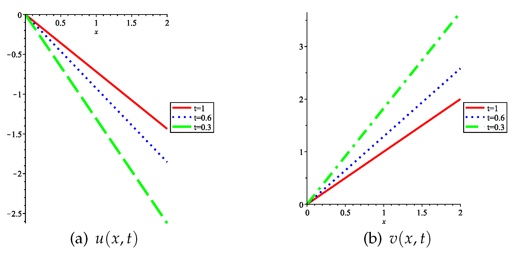
Therefore, an approximated similarity solution to System (1) is given by:

$$\left\{\begin{array}{cc}\hfill u(x,t)& =\left(\frac{1}{2\Gamma (1-\alpha )}-m\right)x{t}^{-\alpha },\hfill \\ \hfill v(x,t)& =mx{t}^{-\alpha },\hfill \end{array}\right.$$

(14)

which is plotted at time $t=1,0.6,0.3$ with $\alpha =\frac{1}{2},m=1$ in Figure 1.

A special approximated similarity solution presents that:

$$\begin{array}{c}\hfill u(x,t)=v(x,t)=\frac{1}{4\Gamma (1-\alpha )}x{t}^{-\alpha }.\end{array}$$

Remark 1.

Similarity solutions of TFBS (1) cannot be obtained by using the similarity variable obtained in [15]. This is the essential difference between the work and that in [15].

For System (9), we can also apply the numerical method to discuss its discrete form and approximated solutions. Assume $\xi \in [1,T+1]$; the grid points are ${\xi }_j=1+jh,h=\frac{T}{N}$. By employing the Taylor formula, we see that:

$$\begin{array}{c}\hfill f({\xi }_j+h)=f\left({\xi }_j\right)+f^{\prime }\left({\xi }_j\right)h+\frac{1}{2}{f}^{″}\left({\xi }_j\right)h^2+o\left(h^2\right),\\ \hfill f({\xi }_j-h)=f\left({\xi }_j\right)-f^{\prime }\left({\xi }_j\right)h+\frac{1}{2}{f}^{″}\left({\xi }_j\right)h^2+o\left(h^2\right),\end{array}$$

from which one gets:

$$\begin{array}{cc}\hfill f^{\prime }\left({\xi }_j\right)& =\frac{f({\xi }_j+h)-f({\xi }_j-h)}{2h}=\frac{f_{j+1}-f_{j-1}}{2h},\hfill \\ \hfill f^{″}\left({\xi }_j\right)& =\frac{f({\xi }_j+h)-2f\left({\xi }_j\right)+f({\xi }_j-h)}{h^2}=\frac{f_{j+1}-2f_j+f_{j-1}}{h^2}.\hfill \end{array}$$

Thus, System (9) can be discretized at point ${\xi }_j$:

$$\left\{\begin{array}{cc}\hfill \frac{F_{j+1}-2F_j+F_{j-1}}{h^2}=& \frac{{\alpha }^2}{4{\xi }_j^2}\left[\frac{1}{\Gamma (1-\alpha )}\frac{F_j}{{\xi }_j^{\alpha }}-2F_j-\left(\frac{6}{\alpha }+\frac{4}{{\alpha }^2}\right){\xi }_j\right.\hfill \\ & \frac{F_{j+1}-F_{j-1}}{2h}+2F_j^2+\frac{2}{\alpha h}{\xi }_j{F}_j(F_{j+1}-F_{j-1})+2F_j{G}_j\hfill \\ & \left.+\frac{1}{\alpha h}{\xi }_j(F_{j+1}-F_{j-1})G_j+\frac{1}{\alpha h}{\xi }_j{F}_j(G_{j+1}-G_{j-1})\right],\hfill \\ \hfill \frac{G_{j+1}-2G_j+G_{j-1}}{h^2}=& \frac{{\alpha }^2}{4{\xi }_j^2}\left[\frac{1}{\Gamma (1-\alpha )}\frac{G_j}{{\xi }_j^{\alpha }}-2G_j-\left(\frac{6}{\alpha }+\frac{4}{{\alpha }^2}\right){\xi }_j\right.\hfill \\ & \frac{G_{j+1}-G_{j-1}}{2h}+2G_j^2+\frac{2}{\alpha h}{\xi }_j{G}_j(G_{j+1}-G_{j-1})+2F_j{G}_j\hfill \\ & \left.+\frac{1}{\alpha h}{\xi }_j(F_{j+1}-F_{j-1})G_j+\frac{1}{\alpha h}{\xi }_j{F}_j(G_{j+1}-G_{j-1})\right].\hfill \end{array}\right.$$

(15)

Choosing $F_{-1}=(\frac{1}{2\Gamma (1-\alpha )}-1)/\sqrt{0.9},F_0=\frac{1}{2\Gamma (1-\alpha )}-1,G_{-1}=1/\sqrt{0.9},G_0=1$ as initial values of system (15), then we can solve (15) by the recurrence procedure, as shown in

Table 1. Solutions of Integer-order ordinary differential equation 1 (IODE-1) with $\alpha =0.5$.

$\mathit{\xi }$	$\mathit{F}\left(\mathit{\xi }\right)$ *	$\mathit{F}\left(\mathit{\xi }\right)$ **	$\mathit{G}\left(\mathit{\xi }\right)$ *	$\mathit{G}\left(\mathit{\xi }\right)$ **
1.1000	−0.6845	−0.6845	0.9535	0.9535
1.2000	−0.6553	−0.6554	0.9129	0.9129
1.3000	−0.6296	−0.6296	0.8770	0.8771
1.4000	−0.6067	−0.6067	0.8451	0.8452
1.5000	−0.5861	−0.5862	0.8165	0.8165
1.6000	−0.5675	−0.5676	0.7905	0.7906
1.7000	−0.5506	−0.5506	0.7669	0.7670
1.8000	−0.5351	−0.5351	0.7453	0.7454
1.9000	−0.5208	−0.5208	0.7254	0.7255
2.0000	−0.5076	−0.5076	0.7070	0.7071

* The numerical solutions of IODE-1 with $T=1,h=0.1$; ** The approximated similarity solutions of Fractional Ordinary Differential System (FODS) (5).

. The error is obviously $O\left(h^2\right)$.

3. Numerical Solutions

In this section, we first investigate the numerical solutions of (1) by making use of the approximated system (8).

According to the method presented in [17,19], we could discuss the numerical solutions of (16) with given initial values. However, we would like to adopt the approach in [25] to introduce discrete equations corresponding to System (8) just like Equation (15), so that we could obtain numerical solutions of System (8). System (8) can be written as follows:

$$\left\{\begin{array}{cc}\hfill F^{″}\left(\xi \right)=& \frac{{\alpha }^2}{4{\xi }^2}\left[-2F\left(\xi \right)-\frac{6\alpha +4}{{\alpha }^2}\xi F^{\prime }\left(\xi \right)+2F^2\left(\xi \right)+\frac{4}{\alpha }\xi F\left(\xi \right)F^{\prime }\left(\xi \right)\right.\hfill \\ & +2F\left(\xi \right)G\left(\xi \right)+\frac{2}{\alpha }\xi F^{\prime }\left(\xi \right)G\left(\xi \right)+\frac{2}{\alpha }\xi F\left(\xi \right)G^{\prime }\left(\xi \right)\hfill \\ & +\frac{\Gamma (3+\alpha )}{2\alpha \Gamma (1-\alpha )\Gamma \left(\alpha \right)}\frac{F\left(\xi \right)}{{\xi }^{\alpha }}-\frac{\alpha }{\Gamma (1-\alpha )}\frac{\left(V_{0}F\right)\left(\xi \right)}{{\xi }^{1+\alpha }}\hfill \\ & \left.-\frac{\Gamma (2+\alpha )}{\Gamma \left(\alpha \right)\Gamma (1-\alpha )\left(\alpha \right)}\frac{\left(V_{1}F\right)\left(\xi \right)}{{\xi }^{2+\alpha }}\right],\hfill \\ \hfill G^{″}\left(\xi \right)=& \frac{{\alpha }^2}{4{\xi }^2}\left[-2G\left(\xi \right)-\frac{6\alpha +4}{{\alpha }^2}\xi G^{\prime }\left(\xi \right)+2G^2\left(\xi \right)+\frac{4}{\alpha }\xi G\left(\xi \right)G^{\prime }\left(\xi \right)\right.\hfill \\ & +2F\left(\xi \right)G\left(\xi \right)+\frac{2}{\alpha }\xi F\left(\xi \right)G^{\prime }\left(\xi \right)+\frac{2}{\alpha }\xi F^{\prime }\left(\xi \right)G\left(\xi \right)\hfill \\ & +\frac{\Gamma (3+\alpha )}{2\alpha \Gamma (1-\alpha )\Gamma \left(\alpha \right)}\frac{G\left(\xi \right)}{{\xi }^{\alpha }}-\frac{\alpha }{\Gamma (1-\alpha )}\frac{\left(V_{0}G\right)\left(\xi \right)}{{\xi }^{1+\alpha }}\hfill \\ & \left.-\frac{\Gamma (2+\alpha )}{\Gamma \left(\alpha \right)\Gamma (1-\alpha )\left(\alpha \right)}\frac{\left(V_{1}G\right)\left(\xi \right)}{{\xi }^{2+\alpha }}\right].\hfill \end{array}\right.$$

(16)

Through the medium-value theorem, the moments $\left(V_{0}F\right)\left(\xi \right),\left(V_{0}G\right)\left(\xi \right),\left(V_{1}F\right)\left(\xi \right)$, and $\left(V_{1}G\right)\left(\xi \right)$ can be expressed approximately as:

$$\begin{array}{c}\hfill \left(V_{0}F\right)\left(\xi \right)\approx \xi F\left(\xi \right),\left(V_{0}G\right)\left(\xi \right)\approx \xi G\left(\xi \right),\left(V_{1}F\right)\left(\xi \right)\approx {\xi }^{2}F\left(\xi \right),\left(V_{1}G\right)\left(\xi \right)\approx {\xi }^{2}G\left(\xi \right).\end{array}$$

Substituting these results into (16) gives rise to:

$$\left\{\begin{array}{cc}\hfill F^{″}\left(\xi \right)=\frac{{\alpha }^2}{4{\xi }^2}& \left\{-2F\left(\xi \right)-\frac{6\alpha +4}{{\alpha }^2}\xi F^{\prime }\left(\xi \right)+2F^2\left(\xi \right)+\frac{4}{\alpha }\xi F\left(\xi \right)F^{\prime }\left(\xi \right)\right.\hfill \\ & +2F\left(\xi \right)G\left(\xi \right)+\frac{2}{\alpha }\xi F^{\prime }\left(\xi \right)G\left(\xi \right)+\frac{2}{\alpha }\xi F\left(\xi \right)G^{\prime }\left(\xi \right)\hfill \\ & \left.+\left[\frac{\Gamma (3+\alpha )}{2\alpha \Gamma (1-\alpha )\Gamma \left(\alpha \right)}-\frac{\alpha }{\Gamma (1-\alpha )}-\frac{\Gamma (2+\alpha )}{\Gamma \left(\alpha \right)\Gamma (1-\alpha )\left(\alpha \right)}\right]\frac{F\left(\xi \right)}{{\xi }^{\alpha }}\right\},\hfill \\ \hfill G^{″}\left(\xi \right)=\frac{{\alpha }^2}{4{\xi }^2}& \left\{-2G\left(\xi \right)-\frac{6\alpha +4}{{\alpha }^2}\xi G^{\prime }\left(\xi \right)+2G^2\left(\xi \right)+\frac{4}{\alpha }\xi G\left(\xi \right)G^{\prime }\left(\xi \right)\right.\hfill \\ & +2F\left(\xi \right)G\left(\xi \right)+\frac{2}{\alpha }\xi F\left(\xi \right)G^{\prime }\left(\xi \right)+\frac{2}{\alpha }\xi F^{\prime }\left(\xi \right)G\left(\xi \right)\hfill \\ & \left.+\left[\frac{\Gamma (3+\alpha )}{2\alpha \Gamma (1-\alpha )\Gamma \left(\alpha \right)}-\frac{\alpha }{\Gamma (1-\alpha )}-\frac{\Gamma (2+\alpha )}{\Gamma \left(\alpha \right)\Gamma (1-\alpha )\left(\alpha \right)}\right]\frac{G\left(\xi \right)}{{\xi }^{\alpha }}\right\}.\hfill \end{array}\right.$$

(17)

Similar to the discussion on Equation (9), we suppose $\xi \in [1,1+T]$; the mean node points are ${\xi }_j=1+jh,h=\frac{T}{N},j=0,1,2,\cdots$. The derivatives of $F\left(\xi \right),G\left(\xi \right)$ can be written as:

$$\begin{array}{c}{F}^{\prime }\left({\xi }_j\right)=\frac{F_{j+1}-F_{j-1}}{2h},F^{″}\left({\xi }_j\right)=\frac{F_{j+1}-2F_j+F_{j-1}}{h^2},\hfill \\ G^{\prime }\left({\xi }_j\right)=\frac{G_{j+1}-G_{j-1}}{2h},G^{″}\left({\xi }_j\right)=\frac{G_{j+1}-2G_j+G_{j-1}}{h^2}.\hfill \end{array}$$

(18)

Using Equation (17) on the points ${\xi }_j$, and inserting (18) into (17), one infers the following discrete equations:

$$\left\{\begin{array}{cc}\hfill \frac{F_{j+1}-2F_j+F_{j-1}}{h^2}=\frac{{\alpha }^2}{4{\xi }_j^2}& \left\{-2F_j-\frac{6\alpha +4}{{\alpha }^2}{\xi }_j\frac{F_{j+1}-F_{j-1}}{2h}+2F_j^2\right.\hfill \\ & +\frac{4}{\alpha }{\xi }_j{F}_j\frac{F_{j+1}-F_{j-1}}{2h}+2F_j{G}_j+\frac{2}{\alpha }{\xi }_j{G}_j\frac{F_{j+1}-F_{j-1}}{2h}\hfill \\ & \left.+\left[\frac{\Gamma (3+\alpha )}{2\alpha \Gamma (1-\alpha )\Gamma \left(\alpha \right)}-\frac{\alpha }{\Gamma (1-\alpha )}-\frac{\Gamma (2+\alpha )}{\Gamma \left(\alpha \right)\Gamma (1-\alpha )}\right]\frac{F_j}{{\xi }_j^{\alpha }}\right\},\hfill \\ \hfill \frac{G_{j+1}-2G_j+G_{j-1}}{h^2}=\frac{{\alpha }^2}{4{\xi }_j^2}& \left\{-2G_j-\frac{6\alpha +4}{{\alpha }^2}{\xi }_j\frac{G_{j+1}-G_{j-1}}{2h}+2G_j^2\right.\hfill \\ & +\frac{4}{\alpha }{\xi }_j{F}_j\frac{G_{j+1}-G_{j-1}}{2h}+2F_j{G}_j+\frac{2}{\alpha }{\xi }_j{F}_j\frac{G_{j+1}-G_{j-1}}{2h}\hfill \\ & \left.+\left[\frac{\Gamma (3+\alpha )}{\alpha \Gamma (1-\alpha )\Gamma \left(\alpha \right)}-\frac{\alpha }{\Gamma (1-\alpha )}-\frac{\Gamma (2+\alpha )}{\Gamma \left(\alpha \right)\Gamma (1-\alpha )}\right]\frac{G_j}{{\xi }_j^{\alpha }}\right\}.\hfill \end{array}\right.$$

(19)

Choosing $F_{-1}=(\frac{1}{2\Gamma (1-\alpha )}-1)/\sqrt{0.9},F_0=\frac{1}{2\Gamma (1-\alpha )}-1,G_{-1}=1/\sqrt{0.9},G_0=1$ as the initial values of System (19), we can obtain some numerical solutions of (19), which are approximated solutions of Equation (5) when $N=2$ (

Table 2. Solutions of IODE-2 with $\alpha =0.5$.

$\mathit{\xi }$	$\mathit{F}\left(\mathit{\xi }\right)$ *	$\mathit{F}\left(\mathit{\xi }\right)$ **	$\mathit{G}\left(\mathit{\xi }\right)$ *	$\mathit{G}\left(\mathit{\xi }\right)$ **
1.1000	−0.6844	−0.6845	0.9533	0.9535
1.2000	−0.6551	−0.6554	0.9125	0.9129
1.3000	−0.6292	−0.6296	0.8765	0.8771
1.4000	−0.6061	−0.6067	0.8443	0.8452
1.5000	−0.5853	−0.5862	0.8153	0.8165
1.6000	−0.5665	−0.5676	0.7891	0.7906
1.7000	−0.5493	−0.5506	0.7652	0.7670
1.8000	−0.5336	−0.5351	0.7433	0.7454
1.9000	−0.5191	−0.5208	0.7231	0.7255
2.0000	−0.5057	−0.5076	0.7045	0.7071

* The numerical solution of IODE-2 with $T=1,h=0.1$; ** the approximated similarity solution of FODS (5).

).

In order to discuss the numerical solutions to System (1), we add another example when $N=3$ in (6) to illustrate the numerical solutions of the FODS (5). When $N=3$, FODS (5) becomes, by using Formula (6),

$$\left\{\begin{array}{c}\frac{\Gamma (4+\alpha )}{6\alpha \Gamma (1-\alpha )\Gamma \left(\alpha \right)}\frac{F\left(\xi \right)}{{\xi }^{\alpha }}-\frac{\Gamma (1+\alpha )}{\Gamma (1-\alpha )\Gamma \left(\alpha \right)}\frac{\left(V_{0}F\right)\left(\xi \right)}{{\xi }^{1+\alpha }}\hfill \\ -\frac{\Gamma (2+\alpha )}{\Gamma (1-\alpha )\Gamma \left(\alpha \right)}\frac{\left(V_{1}F\right)\left(\xi \right)}{{\xi }^{2+\alpha }}-\frac{\Gamma (3+\alpha )}{2\Gamma (1-\alpha )\Gamma \left(\alpha \right)}\frac{\left(V_{2}F\right)\left(\xi \right)}{{\xi }^{3+\alpha }}=P\left(\xi \right),\hfill \\ \frac{\Gamma (4+\alpha )}{6\alpha \Gamma (1-\alpha )\Gamma \left(\alpha \right)}\frac{G\left(\xi \right)}{{\xi }^{\alpha }}-\frac{\Gamma (1+\alpha )}{\Gamma (1-\alpha )\Gamma \left(\alpha \right)}\frac{\left(V_{0}G\right)\left(\xi \right)}{{\xi }^{1+\alpha }}\hfill \\ -\frac{\Gamma (2+\alpha )}{\Gamma (1-\alpha )\Gamma \left(\alpha \right)}\frac{\left(V_{1}G\right)\left(\xi \right)}{{\xi }^{2+\alpha }}-\frac{\Gamma (3+\alpha )}{2\Gamma (1-\alpha )\Gamma \left(\alpha \right)}\frac{\left(V_{2}G\right)\left(\xi \right)}{{\xi }^{3+\alpha }}=Q\left(\xi \right),\hfill \end{array}\right.$$

(20)

where $\left(V_{0}F\right)\left(\xi \right),\left(V_{0}G\right)\left(\xi \right),\left(V_{1}F\right)\left(\xi \right)$, and $\left(V_{1}G\right)\left(\xi \right)$ are the same as those in System (16). We take:

$$\begin{array}{cc}\left(V_{2}F\right)\left(\xi \right)={\int }_0^{\xi }{\tau }^{2}F\left(\tau \right)d\tau \approx {\xi }^{3}F\left(\xi \right),\hfill & \hfill \left(V_{2}G\right)\left(\xi \right)={\int }_0^{\xi }{\tau }^{2}G\left(\tau \right)d\tau \approx {\xi }^{3}G\left(\xi \right).\end{array}$$

Substituting all of results in System (20) yields the following integer-order system of differential equations:

$$\left\{\begin{array}{cc}\hfill F^{″}\left(\xi \right)=\frac{{\alpha }^2}{4{\xi }^2}& \left\{-2F\left(\xi \right)-\frac{6\alpha +4}{{\alpha }^2}\xi F^{\prime }\left(\xi \right)+2F^2\left(\xi \right)+\frac{4}{\alpha }\xi F\left(\xi \right)F^{\prime }\left(\xi \right)+2F\left(\xi \right)G\left(\xi \right)\right.\hfill \\ & +\frac{2}{\alpha }\xi F^{\prime }\left(\xi \right)G\left(\xi \right)+\frac{2}{\alpha }\xi F\left(\xi \right)G^{\prime }\left(\xi \right)+\left[\frac{\Gamma (4+\alpha )}{6\alpha \Gamma (1-\alpha )\Gamma \left(\alpha \right)}\right.\hfill \\ & \left.\left.-\frac{\Gamma (1+\alpha )}{\Gamma (1-\alpha )\Gamma \left(\alpha \right)}-\frac{\Gamma (2+\alpha )}{\Gamma (1-\alpha )\Gamma \left(\alpha \right)}-\frac{\Gamma (3+\alpha )}{2\Gamma (1-\alpha )\Gamma \left(\alpha \right)}\right]\frac{F\left(\xi \right)}{{\xi }^{\alpha }}+2F\left(\xi \right)G\left(\xi \right)\right\},\hfill \\ \hfill G^{″}\left(\xi \right)=\frac{{\alpha }^2}{4{\xi }^2}& \left\{-2G\left(\xi \right)-\frac{6\alpha +4}{{\alpha }^2}\xi G^{\prime }\left(\xi \right)+2G^2\left(\xi \right)+\frac{4}{\alpha }\xi G\left(\xi \right)G^{\prime }\left(\xi \right)\right.\hfill \\ & +\frac{2}{\alpha }\xi F\left(\xi \right)G^{\prime }\left(\xi \right)+\frac{2}{\alpha }\xi F\left(\xi \right)G^{\prime }\left(\xi \right)+\left[\frac{\Gamma (4+\alpha )}{6\alpha \Gamma (1-\alpha )\Gamma \left(\alpha \right)}\right.\hfill \\ & \left.\left.-\frac{\Gamma (1+\alpha )}{\Gamma (1-\alpha )\Gamma \left(\alpha \right)}-\frac{\Gamma (2+\alpha )}{\Gamma (1-\alpha )\Gamma \left(\alpha \right)}-\frac{\Gamma (3+\alpha )}{2\Gamma (1-\alpha )\Gamma \left(\alpha \right)}\right]\frac{G\left(\xi \right)}{{\xi }^{\alpha }}\right\},\hfill \end{array}\right.$$

(21)

which is called IODE-3.

Substituting (18) into (21), we obtain a discrete system:

$$\left\{\begin{array}{cc}\hfill \frac{F_{j+1}-2F_j+F_{j-1}}{h^2}=\frac{{\alpha }^2}{4{\xi }_j^2}& \left\{-2F_j-\frac{6\alpha +4}{{\alpha }^2}{\xi }_j\frac{F_{j+1}-F_{j-1}}{2h}+2F_j^2+\frac{4}{\alpha }{\xi }_j{F}_j\frac{F_{j+1}-F_{j-1}}{2h}\right.\hfill \\ & +2F_j{G}_j+\frac{2}{\alpha }{\xi }_j{G}_j\frac{F_{j+1}-F_{j-1}}{2h}+\left[\frac{\Gamma (4+\alpha )}{6\alpha \Gamma (1-\alpha )\Gamma \left(\alpha \right)}\right.\hfill \\ & \left.\left.-\frac{\Gamma (1+\alpha )}{\Gamma (1-\alpha )\Gamma \left(\alpha \right)}-\frac{\Gamma (2+\alpha )}{\Gamma (1-\alpha )\Gamma \left(\alpha \right)}-\frac{\Gamma (3+\alpha )}{2\Gamma (1-\alpha )\Gamma \left(\alpha \right)}\right]\frac{F_j}{{\xi }_j^{\alpha }}\right\},\hfill \\ \hfill \frac{G_{j+1}-2G_j+G_{j-1}}{h^2}=\frac{{\alpha }^2}{4{\xi }_j^2}& \left\{-2G_j-\frac{6\alpha +4}{{\alpha }^2}{\xi }_j\frac{G_{j+1}-G_{j-1}}{2h}+2G_j^2+\frac{4}{\alpha }{\xi }_j{F}_j\frac{F_{j+1}-F_{j-1}}{2h}\right.\hfill \\ & +2F_j{G}_j+\frac{2}{\alpha }{\xi }_j{G}_j\frac{F_{j+1}-F_{j-1}}{2h}+\left[\frac{\Gamma (4+\alpha )}{6\alpha \Gamma (1-\alpha )\Gamma \left(\alpha \right)}\right.\hfill \\ & \left.\left.-\frac{\Gamma (1+\alpha )}{\Gamma (1-\alpha )\Gamma \left(\alpha \right)}-\frac{\Gamma (2+\alpha )}{\Gamma (1-\alpha )\Gamma \left(\alpha \right)}-\frac{\Gamma (3+\alpha )}{2\Gamma (1-\alpha )\Gamma \left(\alpha \right)}\right]\frac{G_j}{{\xi }_j^{\alpha }}\right\}\hfill \end{array}\right.$$

(22)

Choosing $F_{-1}=(\frac{1}{2\Gamma (1-\alpha )}-1)/\sqrt{0.9},F_0=\frac{1}{2\Gamma (1-\alpha )}-1,G_{-1}=1/\sqrt{0.9},G_0=1$ as initial values of System (22), we can obtain some numerical solutions of (22), which are approximated solutions of FODS (5) when $N=3$ (

Table 3. Solutions of IODE-3 with $\alpha =0.5$.

$\mathit{\xi }$	$\mathit{F}\left(\mathit{\xi }\right)$ *	$\mathit{F}\left(\mathit{\xi }\right)$ **	$\mathit{G}\left(\mathit{\xi }\right)$ *	$\mathit{G}\left(\mathit{\xi }\right)$ **
1.1000	−0.6843	−0.6845	0.9531	0.9535
1.2000	−0.6547	−0.6554	0.9120	0.9129
1.3000	−0.6286	−0.6296	0.8755	0.8771
1.4000	−0.6051	−0.6067	0.8429	0.8452
1.5000	−0.5840	−0.5862	0.8135	0.8165
1.6000	−0.5648	−0.5676	0.7868	0.7906
1.7000	−0.5473	−0.5506	0.7624	0.7670
1.8000	−0.5312	−0.5351	0.7400	0.7454
1.9000	−0.5164	−0.5208	0.7193	0.7255
2.0000	−0.5027	−0.5076	0.7002	0.7071

* The numerical solution of IODE-3 with $T=1,h=0.1$; ** the approximated similarity solution of FODS (5).

).

4. Conclusions

In the paper, we discussed some similarity solutions and some numerical solutions of the TFBS (1) under the case where the time-fractional derivatives are the Riemann–Liouville type. In order to generate similarity solutions, we adopted two approaches, which comprise the Lie-point symmetry method. Thus, two different similarity solutions to the TFBS were obtained. Finally, we investigated some numerical solutions of the TFBS so that we verified the similarity solutions obtained as above with the numerical solutions. The method presented in the paper can be used to study other time-fractional differential systems of equations. Therefore, it has extensive applications. In addition, we could discuss some new symmetries of the TFBS by the developed Lie-group method [14], as well as discuss some conservation laws of the TFBS by using the method presented in [26,27,28]. We would like to further discuss these questions in the forthcoming days.

References

- Kilbas, A.A.; Srivastava, H.M.; Trujillo, J.J. Theory and Applications of Fractional Differential Equations. In North-Holland Mathematics Studies; Elsevier: Amsterdam, The Netherlands, 2006; Volume 204. [Google Scholar]
- Miller, K.S.; Ross, B. An Introduction to the Fractional Calculus and Fractional Differential Equations; Wiley: New York, NY, USA, 1993. [Google Scholar]
- Hilfer, R. Applications of Fractional Calculus in Physics; World Scientific: River Edge, NJ, USA, 2000. [Google Scholar]
- Ortigueira, M.D. Fractional Calculus for Scientists and Engineers; Springer: Amsterdam, The Netherlands, 2011. [Google Scholar]
- Yang, X.J.; Baleanu, D.; Srivastava, H.M. Local Fractional Integral Transforms and their Applications; Academic Press: London, UK, 2016. [Google Scholar]
- Yang, X.J.; Machado, J.A.T.; Srivastava, H.M. A new numerical technique for solving the local fractional diffusion equation: Two-dimensional extended differential transform approach. Appl. Math. Comput. 2016, 274, 143–151. [Google Scholar] [CrossRef]
- Diethelm, K. The Analysis of Fractional Differential Equations; Springer-Verlag: Berlin/Heidelberg, Germany, 2010. [Google Scholar]
- Lakshmikantham, V.; Leela, S.; Devi, J.V. Theory of Fractional Dynamic Systems; CSP: Cambridge, UK, 2009; 170p. [Google Scholar]
- Podlubny, I. Fractional Differential Equations; Academic Press: San Diego, CA, USA, 1999. [Google Scholar]
- Bakkyaraj, T.; Sahadevan, R. Invariant analysis of nonlinear fractional ordinary differential equations with Riemann–Liouville fractional derivative. Nonlinear Dyn. 2015, 80, 447–455. [Google Scholar] [CrossRef]
- Kasatkin, A.A. Symmetry properties for systems of two ordinary fractional differential equations. Ufa Math. J. 2012, 4, 65–75. [Google Scholar]
- Buckwar, E.; Luchko, Y. Invariance of a partial differential equation of fractional order under the Lie group of scaling transformations. J. Math. Anal. Appl. 1998, 227, 81–97. [Google Scholar] [CrossRef]
- Hashemi, M.S. Group analysis and exact solutions of the time fractional Fokker-Plank equation. Phys. A 2015, 417, 141–149. [Google Scholar] [CrossRef]
- Huang, Q.; Shan, S.F. Lie symmetries and group classification of a class of time fractional evolution systems. J. Math. Phys. 2015, 56, 123504. [Google Scholar] [CrossRef]
- Singla, K.; Gupta, R.K. On invariant analysis of some time fractional nonliear systems of partial differential equations I. J. Math. Phys. 2016, 57, 101504. [Google Scholar] [CrossRef]
- Singla, K.; Gupta, R.K. Conservation laws for certain time fractional nonlinear systems of partial differential equations. Commun. Nonlinear Sci. Numer. Simulat. 2017, 53, 10–21. [Google Scholar] [CrossRef]
- Djordjevic, V.D.; Atanackovic, T.M. Similarity solutions to nonlinear heat conduction and Burgers/Kortewge-de Vries fractional equations. J. Comput. Appl. Math. 2008, 222, 701–714. [Google Scholar] [CrossRef]
- Zhang, Y.F.; Mei, J.; Zhang, X. Symmetry properties and explicit solutions of some nonlinear differential and fractional equations. Appl. Math. Comput. 2018, 337, 408–418. [Google Scholar] [CrossRef]
- Atanackovic, T.M.; Stankovic, B. On a numerical scheme for solving differential equations of fractional order. Mech. Res. Commun. 2008, 35, 429–438. [Google Scholar] [CrossRef]
- Atanacković, T.M.; Janev, M.; Konjik, S.; Pilipović, S.; Zorica, D. Expansion formula for fractional derivatives in variational problems. J. Math. Anal. Appl. 2014, 409, 911–924. [Google Scholar] [CrossRef]
- Atanackovic, T.M.; Stankovic, B. An expansion formula for fractional derivatives and its application. Fractional Calculus Appl. Anal. 2004, 7, 365–378. [Google Scholar]
- Lakshmikantham, V.; Vatsala, A.S. Theory of fractional differential inequalities and applications. Commun. Appl. Anal. 2007, 11, 395–402. [Google Scholar]
- Tavares, D.; Almeida, R.; Torres, D.F.M. Caputo derivatives of fractional variable order: Numerical approximations. Commun. Nonlinear Sci. Numer. Simulat. 2016, 35, 69–87. [Google Scholar] [CrossRef] [Green Version]
- Povstenko, Y. Linear Fractional Diffusion-Wave Equation for Scientists and Engineers; Birkhäuser: New York, NY, USA, 2015. [Google Scholar]
- Zhang, Y.F.; Wu, L.X.; Rui, W.J. A corresponding Lie algebra of a reductive homogeneous group and its applications. Commun. Theor. Phys. 2015, 63, 535–548. [Google Scholar] [CrossRef]
- Lukashchuk, S.Y. Conservation laws for time-fractional subdiffusion and diffusion-wave equations. Nonlinear Dynam. 2014, 80, 1–12. [Google Scholar] [CrossRef]
- Ibragimov, N.H. A new conservation theorem. J. Math. Anal. Appl. 2007, 333, 311–328. [Google Scholar] [CrossRef] [Green Version]
- Ibragimov, N.H. Nonlinear self-adjointness and conservation laws. J. Phys. A Math. Theor. 2011, 44, 432002–432010. [Google Scholar] [CrossRef]
Figure 1.
The approximated similarity solution to time-fractional Burgers system (TFBS) at time with .