Enhancement of Curve-Fitting Image Compression Using Hyperbolic Function


1
Computer Engineering Department, College of Engineering, Mustansiriyah University, Baghdad 10047, Iraq
2
Civil Engineering Department, University of Technology, Baghdad 10066, Iraq
*
Author to whom correspondence should be addressed.
Symmetry 2019, 11(2), 291; https://0-doi-org.brum.beds.ac.uk/10.3390/sym11020291
Submission received: 3 December 2018
/
Revised: 6 February 2019
/
Accepted: 21 February 2019
/
Published: 23 February 2019
Abstract
:Image compression is one of the most interesting fields of image processing that is used to reduce image size. 2D curve-fitting is a method that converts the image data (pixel values) to a set of mathematical equations that are used to represent the image. These equations have a fixed form with a few coefficients estimated from the image which has been divided into several blocks. Since the number of coefficients is lower than the original block pixel size, it can be used as a tool for image compression. In this paper, a new curve-fitting model has been proposed to be derived from the symmetric function (hyperbolic tangent) with only three coefficients. The main disadvantages of previous approaches were the additional errors and degradation of edges of the reconstructed image, as well as the blocking effect. To overcome this deficiency, it is proposed that this symmetric hyperbolic tangent (tanh) function be used instead of the classical 1st- and 2nd-order curve-fitting functions which are asymmetric for reformulating the blocks of the image. Depending on the symmetric property of hyperbolic tangent function, this will reduce the reconstruction error and improve fine details and texture of the reconstructed image. The results of this work have been tested and compared with 1st-order curve-fitting, and standard image compression (JPEG) methods. The main advantages of the proposed approach are: strengthening the edges of the image, removing the blocking effect, improving the Structural SIMilarity (SSIM) index, and increasing the Peak Signal-to-Noise Ratio (PSNR) up to 20 dB. Simulation results show that the proposed method has a significant improvement on the objective and subjective quality of the reconstructed image.
1. Introduction
Image processing has been considered to be one of the most important applications of computer engineering in recent decades. It has become one of the pillars of modern technology, and consists of several branches that work to improve image quality [1], image retrieval [2], image restoration [3], and image compression [4], which is considered to be the most important branch as it deals with reducing the size of the image. Due to the large increase of data and information, including the increased volumes of digitized medical information, hyperspectral, and digital images, the challenge now is how to deal with the storage and transmission requirements. This is why image and data compression is still considered an effective research field [5,6].
The purpose of image compression is to minimize image size while retaining maximum information considering the human eye abilities such as a low sensitivity of distinguishing colors. For example, the uncompressed colored image BMP contains (more than 16 million) colors while the human eye can only distinguish up to 256 color levels. Therefore, high accuracy color information will not be sensed by the human eye, thus, image size can be reduced and therefore this can be considered to be the basic principle of image compression [1].
In general, image compression methods are divided into two categories; lossless and lossy methods. Lossless methods maintain image pixels without any loss, i.e., the original image can be completely recovered after the decompression process. TIFF (Tagged Image File Format), LZW (Lempel-Ziv-Welch), and PNG (Portable Network Graphics) are examples of these methods that are suitable for web browsing, image editing, and printing. Lossy methods benefit from the inherent redundancies of the image, such as psycho-visual redundancy, inter-pixel redundancy, or coding redundancy to reduce the amount of data needed to represent the image, i.e., the original image cannot be completely recovered. Therefore, lossy methods give high compression ratios with low signal-to-noise ratios (PSNR). JPEG is an example of this approach, which is a suitable method for most images [7].
Furthermore, image compression can be implemented into two domains, namely spatial and frequency. In the spatial domain, the digital image is decomposed into its bit-planes [8], and the process detects how to ignore some of these pixels without affecting the resulting image [9]. In the frequency domain a discrete transform such as Discrete Cosine transform (DCT), Fourier Transform (FT), or Wavelet Transform (WT) that can be applied to compact the energy of the image into only few coefficients, while low coefficients can be set to zero, followed by quantization and entropy coding, such as Huffman coding method, to reduce the number of bits required to represent pixel value (bpp) [10].
Curve-fitting has been used in different image processing algorithms, such as image compression through plane fitting [11], block-based piecewise linear image coding using surface triangulation [12], image representation and creation based on curvilinear feature driven subdivision surfaces [13], segmentation-based compression using modified competitive learning network [14], as well as segmentation-based gray image compression through global approximations of sub-images by 2D polynomial along with corrections [15].
During the last two decades, image compression methods in the spatial domain have been developed using 2D curve-fitting, which essentially transforms the image from random values to simple mathematical equations (linear or non-linear) [2]. 2D curve-fitting depends on dividing the image into blocks of pixels, which are converted into a set of equations. Thus, it can reduce the size of the storage space and save only a few coefficients of the equation that represent the blocks of image. This is the essential idea of this image compression approach [2,11,13].
Ameer and Basir implemented a scalable image compression scheme via plane fitting by dividing the image into non-overlapping blocks (typically of pixels) and presented each block with only three or four quantized coefficients. The block center was chosen as the origin followed by simple quantization and coding schemes to reduce the cost [16]. Sadanandan and Govindan proposed a lossy compression method to eliminate the redundancy in the image using two steps, namely skip line encoding and curve-fitting-based encoding [17]. Liu and Peng proposed a rotating mapping curve-fitting algorithm for image compression; this method depends on the correlation of the DC component and the rotation angle between adjacent blocks. They have proven that lots of blocks need less curve-fitting data to fit the AC component [18]. Sajikumar and Anilkumar proposed bivariate polynomial surface fitting for image compression. Chebyshev polynomials of first kind were used to generate the surface for each block; this method stores three to four parameters of the fitted surface at each block instead of pixel values. Therefore, its compression ratio did not depend on redundant information but depended on a predefined block size [19]. Al-Bahadili proposed a method that depended on the value of block-pixels variance to apply two adaptive polynomial fittings for image compression combined with uniform quantizer and Huffman encoding, the variance value of each block determined the minimum number of coefficients for each block [20]. Image compression using curve-fitting has applied on wireless multimedia sensor networks (WMSNs) for energy saving [21] and has been applied for intra-prediction coding modality of High-Efficiency Video Coding (HEVC) using a piecewise mapping (pwm) function [22]. Hyperspectral image compression using Savitzky-Golay smoothing filter with curve-fitting model is presented in [23]. Butt and Sattar proposed a curve-fitting model for image compression in [24]. This study discussed a comparison using and block sizes at 1st- and 2nd-order curve and showed that there was a large difference in compression ratio for the same value of mean squared error or Peak Signal-to-Noise Ratio (PSNR). Using block size has given better quality of images in comparison to block size at the same curve-fitting order but less compression ratio [24].
Image compression using curve-fitting has many disadvantages and artifacts. Thus, it is still not widely used, but it is a promising and scalable method for research. This paper aims to improve the results that depend only on curve-fitting approach without applying any smoothing filter [23], segmentation algorithms [14], defining some polygon vertices [11,12,13], or without applying coding technique to the parameters [12,21,22]. It uses a non-linear function which is more flexible than previous proposed curve-fitting or interpolation functions, which incorporates better edge and texture description. The proposed function model focuses on solving the problem of edge distortion of the decompressed image to get an image that is very similar to the original one.
The main weaknesses in all previously mentioned curve-fitting functions (linear or non-linear) in the related work are the edge quality (fine features) of the image and the blocking effects of the reconstructed image. Some works proposed a post-processing [16,19] or pre-processing process [13] to reduce these imperfections; however, this paper proposes an able curve-fitting function to maintain the fine details of compressed image.
2. 2D Curve-Fitting of Image
Curve-fitting refers to the use of a mathematical expression to represent gathered random data into a group. This data has one or two dimensions. The 2-dimensional (2D) data is represented by a matrix of data such as the digital image that is saved and processed. This duality means that the image or block (small part) of the image () can be represented as a 2D mathematical expression ().
To achieve data compression, least squares approximation was presented as an optimization algorithm where only a small number of coefficients is enough to represent all pixels in the block of the image. Mathematically, we have
where is the original intensity value of the image (or any color component) and is the value from the suggested function. A simplified derivation of first order (plane) fitting was proposed by [24] as the following
The coefficients a, b, and c of a block are computed from their counter parts and were assumed uniformly distributed. The resulting values of the minimization procedure, usually or , were retained whenever the resulting error was less than a prescribed threshold. A PSNR of 32 dB was reported for 16:1 compression (0.5 bpp) with high complexity in building the quad tree describing the sizes of the compressed blocks. To reduce the error energy imposed by quantizing a and b, the block center was selected as the origin of the coordinate system. In fact, the selection of the origin can also affect the range values of c [25,26].
3. The Proposed Method
In the abovementioned works, different functions (linear and non-linear) for 2D curve-fitting were used. These functions have satisfied good subjective results for the general view of the image, but the main drawback was the subjective quality (edges of the image). However, some works proposed special processes [13,14,16,19] to resolve the edges and texture description problem, but these processes have reduced PSNR and increased the image reconstruction time.
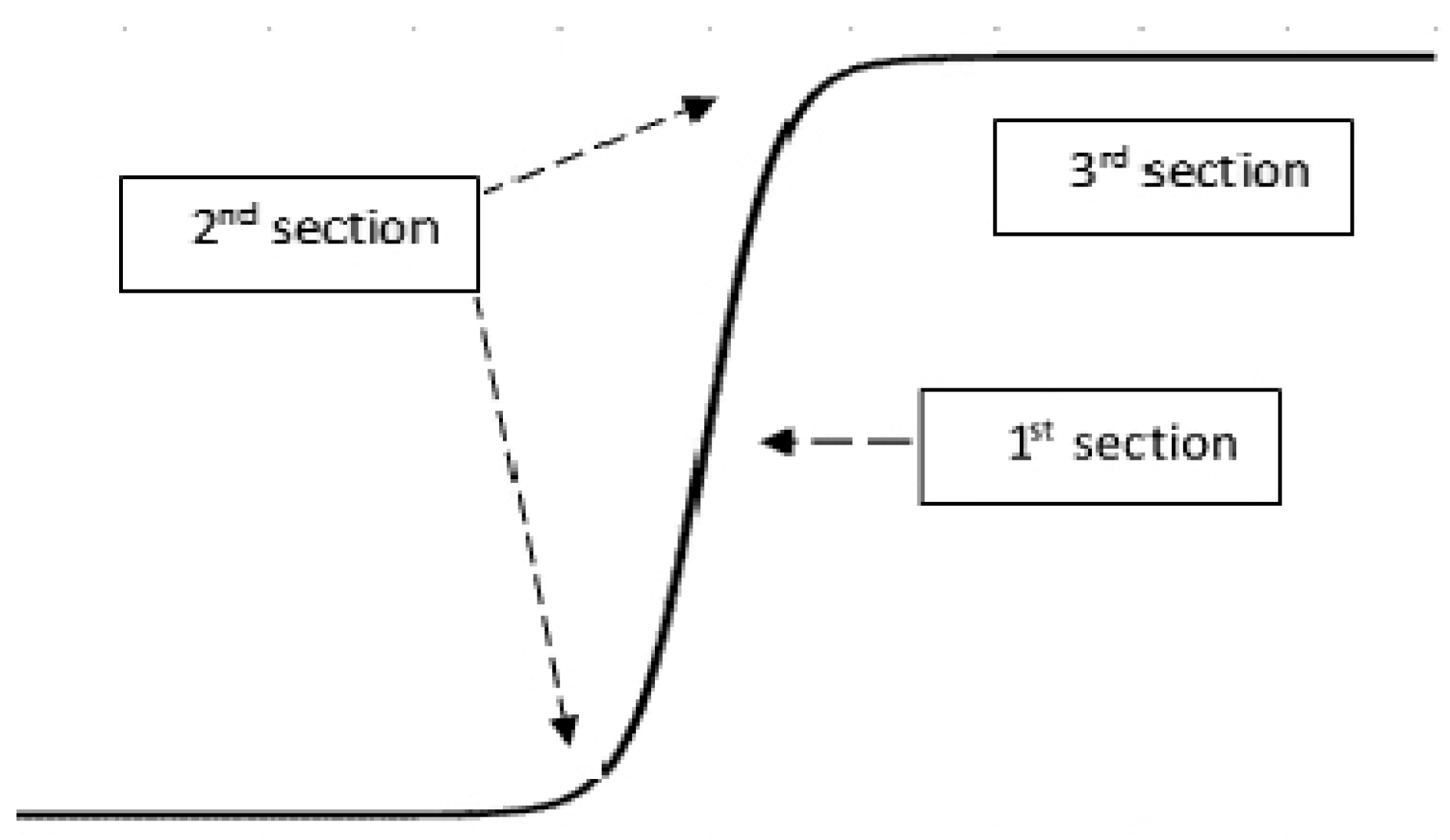
In this paper, a 2D curve-fitting function for image compression is proposed to maintain edges and texture of the reconstructed image. This function is a hyperbolic tangent (), and is a non-linear function that has three main sections as shown in Figure 1; the first section is a semi-linear function that works with the growing area in the image (block), the second section works with edges, while the third section is a flat part that works with flat area in the image.
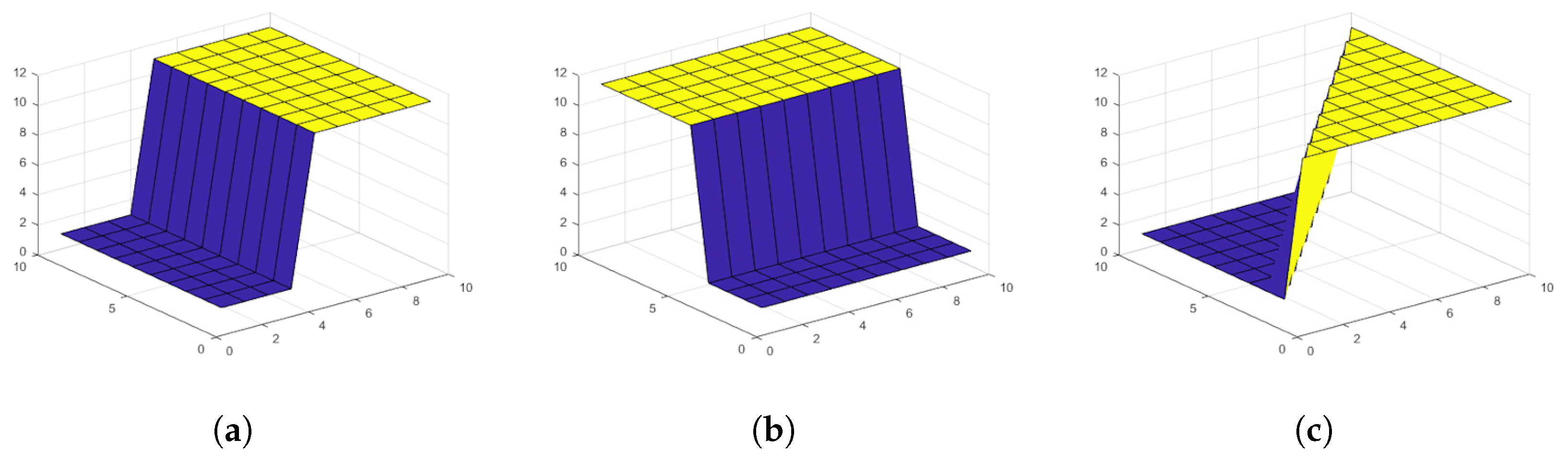
In general, image representation is a 2D matrix (surface); therefore, the proposed function is modified for a 2D function of 4 coefficients, as shown in Equation (3). The image is divided into blocks; each block contains a maximum of one edge type as shown in Figure 2.
where a is the base value of the block (minimum value), b is the growing parameter, while c and d are controlling the edge orientation in the block. The edge orientation changes slowly for large coefficients (c or d), the condition in Equation (4) is for achieving perceptible orientation change, the maximum value of tanh function is 0.964 () at the end corner of the block , this condition will shrink the values of these coefficients and reduce the number of coefficients to three, which as a result, will increase the Compression Ratio (CR).
To represent the image using Equations (3) and (4), their coefficients (, and d) need to be calculated. First, we divide the image into blocks, each one consists of points, then we save the block corner values as ( and ), and finally we rotate the block to move the minimum corner value at the left bottom corner ().
The rotated block is then called , this block is then used to calculate the coefficients and d as follows:
Hence, the calculated coefficients are considered as initial values and are used to find the final values of these coefficients as in Equation (1), which reduces the error between the estimated values () and the actual values (), these coefficients are then codded and saved in three separate matrices which are called , , and .
The decompression process uses these matrices to re-generate the blocks and re-rotate them to the correct position, then grouping them in one matrix (image). A simple post-processing technique could be used to enhance the final result (final image).
3.1. Simple Block Compression Algorithm
A simple case for the proposed work using block size can be described in the following four main steps. The first step is pre-processing, the second step is calculating the initial values of the coefficients, which will be used to find the final values of these coefficients ( and d), and the third step is the enhancement of these values using Equation (1), while coding these coefficients will be implemented in the fourth step.
Step 1: pre-processing
- Find t(1,1) : .
- Find l(1,1) : .
- Limitation, using Equation (10) for each pixel point in this block
Step 2: initial values
- Rotate the block to satisfy (minimum corner at ) then find and
- Find initial values of and d asAdding 1 to the denominator to avoid dividing by zero.
Step 3: values enhancement
- Calculate the values of for and using Equation (3) for each pixel point of the block.
- Calculate the error using Equation (11):
- Repeat 1, 2 and 3 while
Step 4: coding
,
,
.
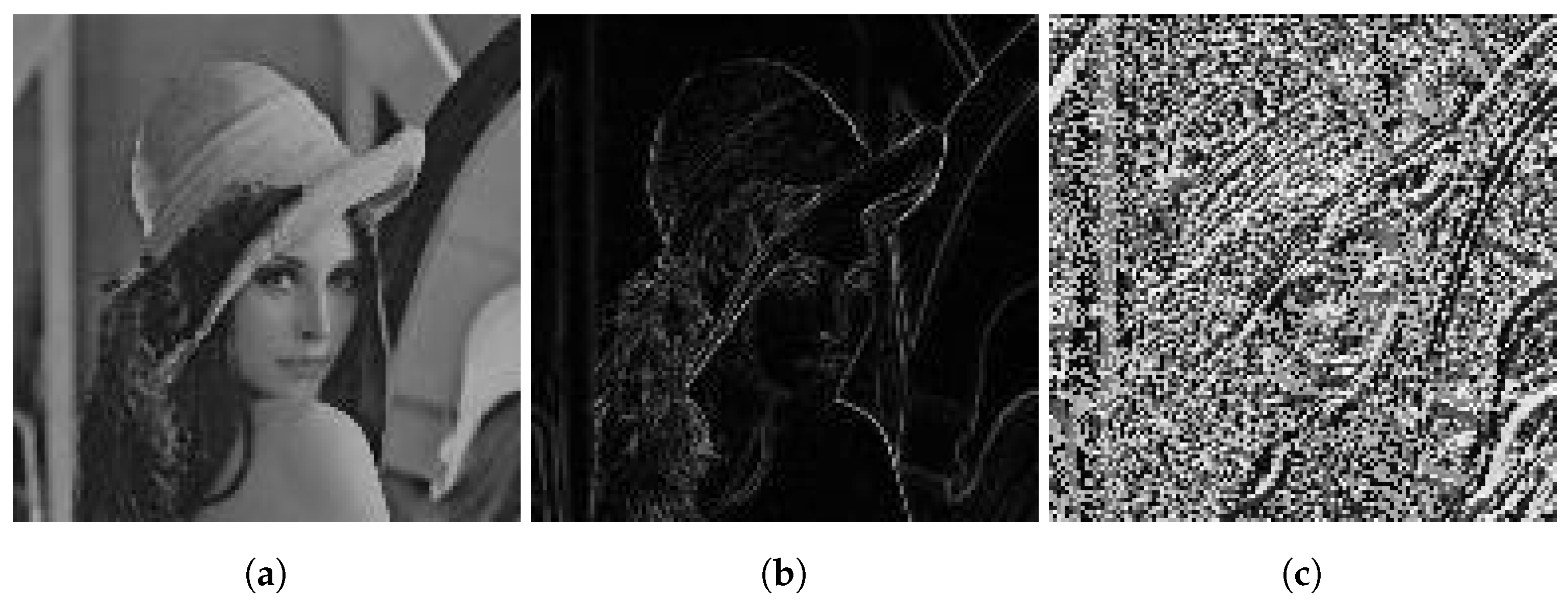
Hence, Figure 3 shows an example for these matrices.
3.2. Simple Block Decompression Algorithm
The decompression process is simple and fast and comprises of two steps, representing the inverse of Step 4 and Step 2 of the compression side, as follows:
Step 1: decoding
Find and d as follows:
,
,
,
,
,
.
Step 2: block values calculation
- Calculate the values of for and using Equation (3) for each point of the block.
- Re-rotate the block using the values of and .
4. Experimental Results
Image compression quality can be assessed using three main factors, which are CR, PSNR, and Structural Similarity Index (SSIM) [13,21]. Image CR can be defined as [2]:
PSNR is defined as [2].
where g and are the original and reconstructed image pixel value respectively, and , where X and Y are image dimensions.
Structural Similarity Index (SSIM) measures the range of structural variation of reconstructed image over original one [13,21]. Its value ranges between 0.0–1.0, higher value means small structural variation, and vice versa.
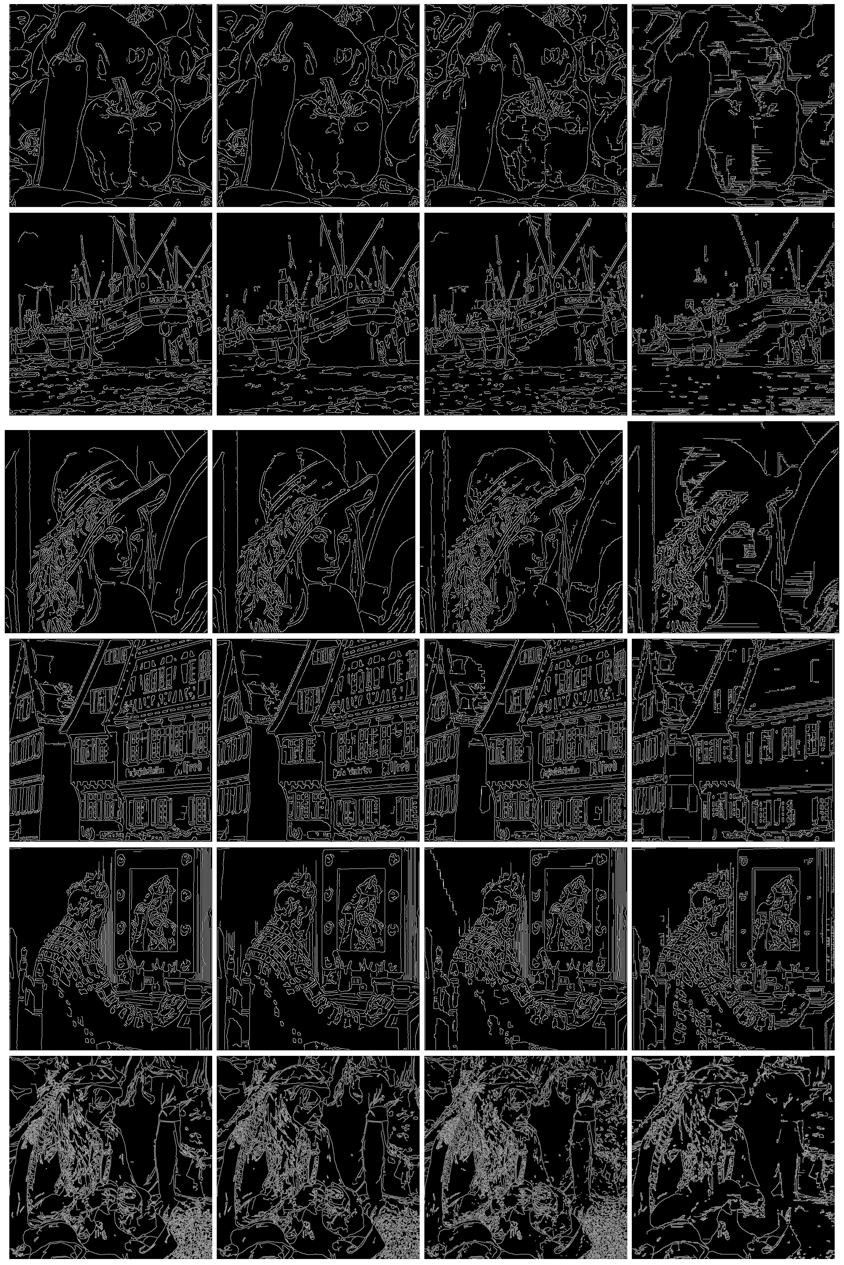
Optimum edge detection of the image can be considered to be an important factor for defining subjective image quality, therefore; in this manuscript, edge detection test will be considered as another measurement for image compression quality.
Applying 1st-order curve-fitting using block size gave better quality than using block size, and it gave better image quality than (or ) block size when 2nd-order curve-fitting was applied [16,26]. Therefore, the test process in our experimental work will use block size applying 1st order for comparison purposes.
The CR result will be the same value for all tested images, because each block consists of 16 pixels (each one of 8-bits) and the result is consisting of three coefficients (each one of 8-bits), then the CR = 16:3 = 5.3:1 without quantization and entropy coding, while using them the CR value could reach 14:1 [4].
4.1. Objective Test (PSNR)
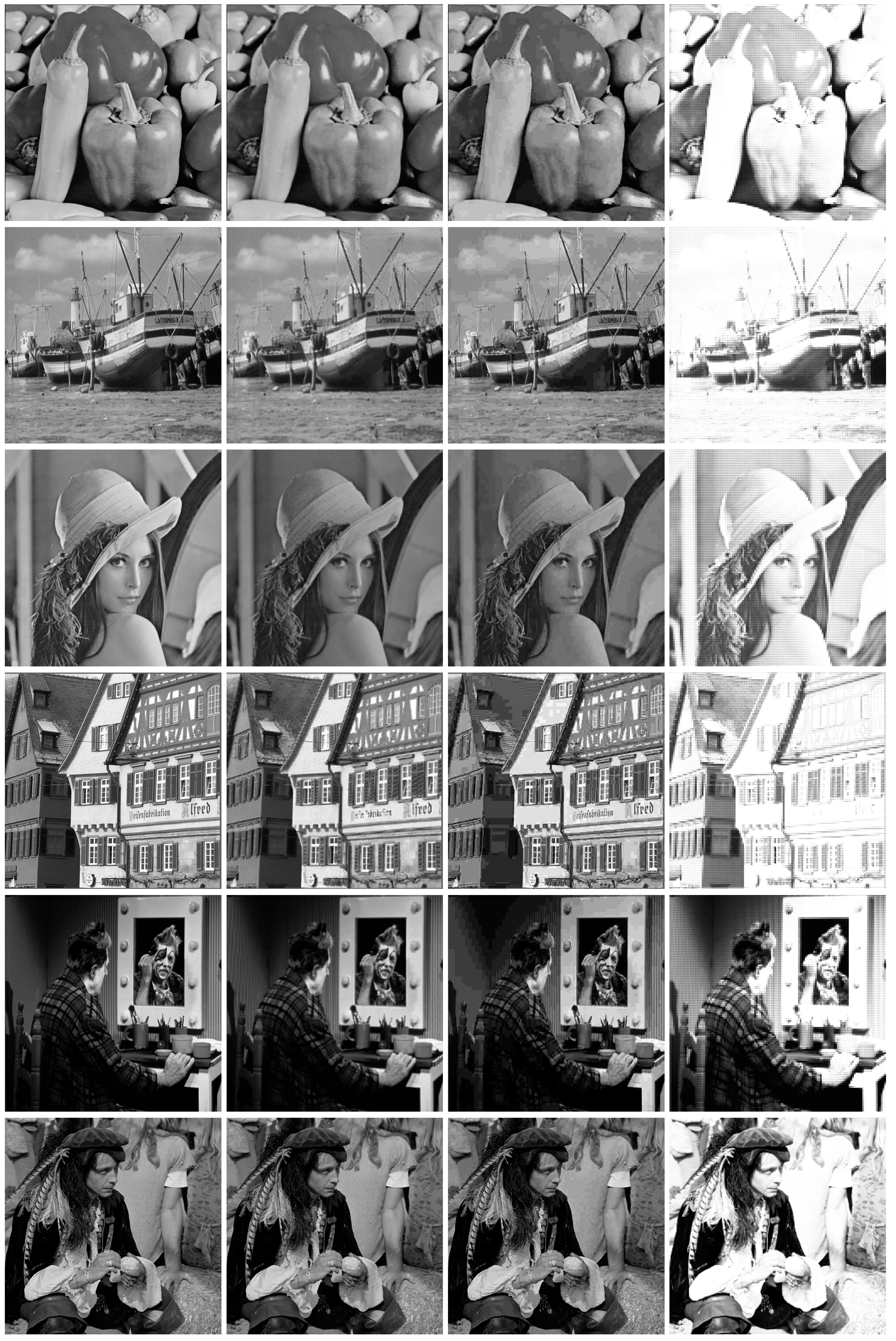
The first test compares the PSNR of six standard test images (PEPPER, BOAT, LENA, HOUSES, CLOWN, and MAN), Figure 4 shows CR results of the six test images using the proposed method and 1st order method, while PSNR and MSE results are listed in Table 1.
From Table 1 we can note that the proposed method (tanh function) increased the average of the PSNR from 8.5 dB to 29.7 dB under same conditions. This test uses block size without quantization and entropy coding and without applying any pre-processing.
4.2. Subjective Test (Edges)
The subjective test is comprised of edge detection and SSIM index. Edge detection test compares the edge sharpness of six test images that have been used in the objective test, the results are shown in Figure 5. From this figure, we note that the proposed method enhances the edges of the reconstructed image and removes the blocking effects. To evaluate our compression quality, we have used SSIM index which evaluates the human subjective assessment [13], Table 2 shows the SSIM results of the proposed method and JPEG for same objective quality (PSNR).
From this table, it is observed that the proposed method has better SSIM results than JPEG, although they have same PSNR (obviously, the CR of JPEG is higher than the recent proposed method which does not use any quantization or entropy coding, but we have to recall that JPEG uses quantization and Huffman coding, which accomplished most of this CR).
Table 3 shows the SSIM and PSNR results of the proposed method and JPEG for the same CR which is 5.3, to realize a fair comparison between the proposed method and JPEG, neither quantization nor Huffman coding are applied to JPEG.
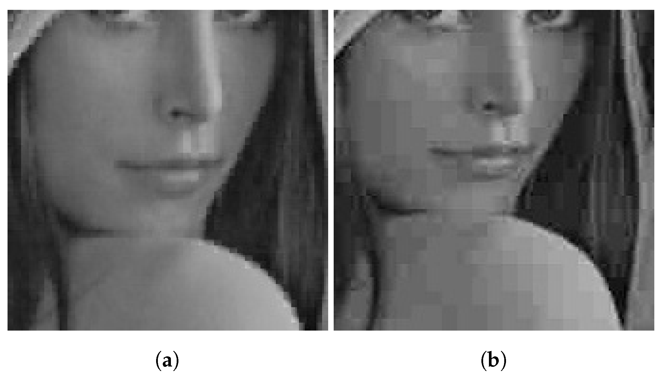
Figure 6 shows an example of image magnification based on our method and JPEG method. We can see that the image features are well preserved and without blocking effects when the proposed method is applied in comparison with JPEG for the same PSNR.
Table 1, Table 2 and Table 3 and Figure 4, Figure 5 and Figure 6 represent results of using only the curve-fitting function without any quantization and entropy coding or post-processing. The CR can be increased using quantization and entropy coding techniques [29] as in JPEG, so these results could be enhanced using post-processing filters [30,31] to reduce the blocking effects which are introduced through compression steps.
5. Conclusions
This manuscript presents a lossy compression method based on curve-fitting using the hyperbolic tangent function. Simulation results showed that the use of hyperbolic tangent function has increased the objective image quality (PSNR) by 20 dB in comparison with 1st-order curve-fitting function ( block size), and has improved the subjective image quality (SSIM increased up to 10%) by removing the blocking effects and enhancing the edge and texture description in comparison with standard image compression method (JPEG) for the same PSNR, as well as both objective and subjective image quality of the reconstructed image using the proposed method is more satisfactory than JPEG for the same CR and neither quantization nor Huffman coding are used.
The proposed method is efficient for high-quality grayscale images, so it can be modified to RGB images and expanded to block size to increase CR from 5.3:1 to 21.3:1 without quantization and entropy coding. The results of the 2D curve-fitting for high-quality colored images and block size using hyperbolic tangent function and suitable quantization could compete with the CR of the JPEG method. Applying some smoothing filters on image data or increasing the size of block to or to improve the CR are part of our extensions for future work.
Author Contributions
Conceptualization, W.K. and D.Z.; Methodology, D.Z.; Software, N.H.; Validation, W.K., D.Z. and N.H.; Formal Analysis, D.Z.; Investigation, N.H.; Resources, W.K.; Data Curation, N.H.; Writing—Original Draft Preparation, D.Z.; Writing—Review and Editing, W.K.; Visualization, N.H.; Supervision, D.Z.
Funding
This research received no external funding.
Acknowledgments
We would like to present our thanks to Mustansiriyah university for supporting our experiments in providing us all the necessary data and software.
Conflicts of Interest
The authors declare no conflict of interest.
Abbreviations
The following abbreviations are used in this manuscript:
| CR | Compression Ratio |
| MSE | Mean Squared Error |
| PSNR | Peak Signal-to-Noise Ratio |
| SSIM | Structural Similarity Index |
| bpp | bits per pixel |
References
- Li, P.; Shen, H.; Zhang, L. A Method of Image Resolution Enhancement Based on the Matching Technique. Available online: http://www.isprs.org/proceedings/xxxv/congress/comm3/papers/356.pdf (accessed on 10 October 2018).
- Mussarat, Y.; Sajjad, M.; Muhammad, S. Intelligent image retrieval techniques: A survey. J. Appl. Res. Technol. 2014, 12, 87–103. [Google Scholar] [CrossRef]
- Alsayem, H.A.; Kadah, Y.M. Image restoration techniques in super-resolution reconstruction of MRI images. In Proceedings of the 2016 33rd National Radio Science Conference (NRSC), Aswan, Egypt, 22–25 February 2016; pp. 188–194. [Google Scholar]
- Bharti, P.; Gupta, S.; Bhatia, R. Comparative analysis of image compression techniques a case study on medical images. In Proceedings of the IEEE International Conference on Advances in Recent Technologies in Communication and Computing, Kottayam, Kerala, India, 27–28 October 2009; pp. 820–822. [Google Scholar]
- Liu, F.; Hernandez-Cabronero, M.; Sanchez, V.; Marcellin, M.W.; Bilgin, A. The current role of image compression standards in medical imaging. Information 2017, 8, 131. [Google Scholar] [CrossRef]
- Al-Bastaki, Y.A. Adaptive GIS Image Compression and Restoration Using Neural Networks. Math. Comput. Appl. 2003, 8, 191–200. [Google Scholar] [CrossRef]
- Gonzalez, R.C.; Woods, R.E. Digital Image Processing, 3rd ed.; Prentice-Hall, Inc.: Upper Saddle River, NJ, USA, 2006; ISBN 013168728X. [Google Scholar]
- Kabir, M.A.; Mondal, M.R.H. Edge-based and prediction-based transformations for lossless image compression. J. Imaging 2018, 4, 64. [Google Scholar] [CrossRef]
- Hassan, S.A.; Hussain, M. Spatial domain lossless image data compression method. In Proceedings of the International Conference on Information and Communication Technologies, Karachi, Pakistan, 23–24 July 2011; pp. 1–4. [Google Scholar]
- Miklos, P. Comparison of spatial and frequency domain image compression methods. In Proceedings of the 4th International Conference and Workshop Mechatronics in Practice and Education, Subotica, Serbia, 4–5 May 2017; pp. 57–60. [Google Scholar]
- Watanabe, T. Picture coding employing b-spline surfaces with multiple vertices. Electron. Comm. Jpn. Part I 1997, 80, 50–65. [Google Scholar] [CrossRef]
- Lu, T.; Le, Z.; Yun, D. Piecewise linear image coding using surface triangulation and geometric compression. In Proceedings of the 2000 Data Compression Conference (DCC), Snowbird, UT, USA, 28–30 March 2000; pp. 410–419. [Google Scholar]
- Zhou, H.; Zheng, J.; Wei, L. Representing images using curvilinear feature driven subdivision surfaces. IEEE Trans. Image Process. 2014, 23, 3268–3280. [Google Scholar] [CrossRef]
- Hsu, W.; Chen, K. Segmentation-based compression using modified competitive network. J. Med. Biol. Eng. 2014, 34, 542–546. [Google Scholar] [CrossRef]
- Biswas, S. Segmentation based compression for gray level images. Pattern Recognit. 2003, 36, 1501–1517. [Google Scholar] [CrossRef]
- Ameer, S.; Basir, O. Image compression using plane fitting with inter-block prediction. Image Vis. Comput. 2009, 27, 385–390. [Google Scholar] [CrossRef]
- Sadanandan, S.; Govindan, V.K. Image compression with modified skip line encoding and curve fitting. Int. J. Comput. Appl. 2013, 74, 24–30. [Google Scholar]
- Liu, Y.; Peng, S. A new image compression algorithm base on rotating mapping and curve fitting. In Proceedings of the 12th International Conference on Signal Processing (ICSP), Hangzhou, China, 19–23 October 2014; pp. 934–937. [Google Scholar]
- Sajikumar, S.; Anilkumar, A.K. Image compression using chebyshev polynomial surface fit. Int. J. Pure Appl. Math. Sci. 2017, 10, 15–27. [Google Scholar]
- Al-Bahadili, R. Adaptive polynomial fitting for image compression based on variance of block pixels. Eng. Technol. J. 2015, 33, 1830–1844. [Google Scholar]
- Banerjee, R.; Das Bit, S. An energy efficient image compression scheme for wireless multimedia sensor network using curve fitting technique. Wirel. Netw. 2017, 25, 167–183. [Google Scholar] [CrossRef]
- Sanchez, V.; Aulí-Llinàs, F.; Serra-Sagristà, J. Piecewise mapping in HEVC lossless intra-prediction coding. IEEE Trans. Image Process. 2016, 25, 4004–4017. [Google Scholar] [CrossRef] [PubMed]
- Beitollahi, M.; Hosseini, S.A. Using savitsky-golay smoothing filter in hyperspectral data compression by curve fitting. In Proceedings of the 26th Iranian Conference on Electrical Engineering (ICEE), Mashhad, Iran, 8–10 May 2018; pp. 452–557. [Google Scholar]
- Butt, A.M.; Sattar, R.A. On Image Compression Using Curve Fitting. Master’s Thesis, The Blekinge Institute of Technology, Karlskrona, Sweden, 2010. [Google Scholar]
- Strobach, P. Quadtree-structured recursive plane decomposition coding of images. IEEE Trans. Signal Process. 1991, 39, 1380–1397. [Google Scholar] [CrossRef]
- Ameer, S. Investigating Polynomial Fitting Schemes for Image Compression. Ph.D. Thesis, University of Waterloo, Waterloo, ON, Canada, 2009. [Google Scholar]
- Philips, W. Recursive computation of polynomial transform coefficients. Electron. Lett. 1991, 27, 2337–2339. [Google Scholar] [CrossRef]
- Hasegawa, M.; Yamasaki, I. Image data compression with nonuniform block segmentation and luminance approximation using bilinear curved surface patches. Syst. Comput. Jpn. Banner 2002, 33, 31–40. [Google Scholar] [CrossRef]
- Shi, C.; Wang, L.; Zhang, J.; Miao, F.; He, P. Remote Sensing Image Compression based on direction lifting-based block transform with content-driven Quadtree coding adaptively. Remote Sens. 2018, 10, 999. [Google Scholar] [CrossRef]
- AL Wahab, D.S.; Zaghar, D.; Laki, S. FIR Filter design based neural network. In Proceedings of the 11th International Symposium on Communication Systems, Networks, and Digital Signal Processing (CSNDSP 2018), Budapest, Hungary, 18–20 July 2018; pp. 1–4. [Google Scholar]
- Yu, C.-Y.; Lin, C.-Y.; Yang, S.-C.; Lin, H.-Y. Eight-scale image contrast enhancement based on adaptive inverse hyperbolic tangent algorithm. Algorithms 2014, 7, 597–607. [Google Scholar] [CrossRef]
Figure 1.
One dimensional function.

Figure 2.
Some examples of 2D function. (a): Vertical Edge; (b): Horizontal Edge; (c): Diagonal Edge.
Figure 2.
Some examples of 2D function. (a): Vertical Edge; (b): Horizontal Edge; (c): Diagonal Edge.

Figure 3.
Results of Compression Method. (a): result of matrix a; (b): result of matrix b; (c): result of matrix c.
Figure 3.
Results of Compression Method. (a): result of matrix a; (b): result of matrix b; (c): result of matrix c.

Figure 4.
The first column: original images; the second column: results of proposed method; the third column: results of JPEG method, the fourth column: results of 1st-order curve-fitting.
Figure 4.
The first column: original images; the second column: results of proposed method; the third column: results of JPEG method, the fourth column: results of 1st-order curve-fitting.

Figure 5.
The first column: original images edge detection; the second column: results of edge detection for proposed method; the third column: results of edge detection for JPEG method; the fourth column: results of edge detection for 1st order curve-fitting.
Figure 5.
The first column: original images edge detection; the second column: results of edge detection for proposed method; the third column: results of edge detection for JPEG method; the fourth column: results of edge detection for 1st order curve-fitting.

Figure 6.
Image magnification . (a): our method; (b): JPEG method.


Table 1.
Objective test (PSNR) results.
| Image Name | PEPPER | BOAT | LENA | HOUSES | CLOWN | MAN |
|---|---|---|---|---|---|---|
| size | 257 K | 257 K | 257 K | 257 K | 257 K | 1 M |
| MSE of proposed method | 64 | 117 | 37 | 448 | 81 | 83 |
| MSE of 1st order | 8793 | 9643 | 1025 | 9265 | 4606 | 7867 |
| PSNR of proposed method | 30.10 | 27.4 | 32.50 | 21.6 | 29.0 | 28.90 |
| PSNR of 1st order | 8.70 | 8.30 | 8.02 | 8.46 | 11.49 | 9.17 |
Table 2.
Subjective test (SSIM index) results.
| Image Name | PEPPER | BOAT | LENA | HOUSES | CLOWN | MAN |
|---|---|---|---|---|---|---|
| PSNR | 30.1 | 27.4 | 32.5 | 21.6 | 29.0 | 28.9 |
| Proposed method | 0.8420 | 0.7931 | 0.8917 | 0.7142 | 0.8525 | 0.8160 |
| JPEG | 0.7849 | 0.7347 | 0.8633 | 0.6601 | 0.7342 | 0.7462 |
Table 3.
Objective and subjective test results for the same CR (5.3). ( Neither quantization nor Huffman coding are used.)
Table 3.
Objective and subjective test results for the same CR (5.3). ( Neither quantization nor Huffman coding are used.)
| Method | PEPPER | BOAT | LENA | HOUSES | CLOWN | MAN | |
|---|---|---|---|---|---|---|---|
| JPEG 1 | PSNR | 29.9 | 27.8 | 32.0 | 22.5 | 29.5 | 29.7 |
| SSIM | 0.7849 | 0.7347 | 0.8633 | 0.6601 | 0.7342 | 0.7462 | |
| Proposed | PSNR | 30.1 | 27.4 | 32.5 | 21.6 | 29.0 | 28.9 |
| SSIM | 0.8420 | 0.7931 | 0.8917 | 0.7142 | 0.8525 | 0.8160 |
© 2019 by the authors. Licensee MDPI, Basel, Switzerland. This article is an open access article distributed under the terms and conditions of the Creative Commons Attribution (CC BY) license (http://creativecommons.org/licenses/by/4.0/).
Share and Cite
MDPI and ACS Style
Khalaf, W.; Zaghar, D.; Hashim, N. Enhancement of Curve-Fitting Image Compression Using Hyperbolic Function. Symmetry 2019, 11, 291. https://0-doi-org.brum.beds.ac.uk/10.3390/sym11020291
AMA Style
Khalaf W, Zaghar D, Hashim N. Enhancement of Curve-Fitting Image Compression Using Hyperbolic Function. Symmetry. 2019; 11(2):291. https://0-doi-org.brum.beds.ac.uk/10.3390/sym11020291
Chicago/Turabian StyleKhalaf, Walaa, Dhafer Zaghar, and Noor Hashim. 2019. "Enhancement of Curve-Fitting Image Compression Using Hyperbolic Function" Symmetry 11, no. 2: 291. https://0-doi-org.brum.beds.ac.uk/10.3390/sym11020291
Note that from the first issue of 2016, this journal uses article numbers instead of page numbers. See further details here.