Stability Analysis of Darcy-Forchheimer Flow of Casson Type Nanofluid Over an Exponential Sheet: Investigation of Critical Points

Abstract

In this paper, steady two-dimensional laminar incompressible magnetohydrodynamic flow over an exponentially shrinking sheet with the effects of slip conditions and viscous dissipation is examined. An extended Darcy Forchheimer model was considered to observe the porous medium embedded in a non-Newtonian-Casson-type nanofluid. The governing equations were converted into nonlinear ordinary differential equations using an exponential similarity transformation. The resultant equations for the boundary values problem (BVPs) were reduced to initial values problems (IVPs) and then shooting and Fourth Order Runge-Kutta method (RK-4th method) were applied to obtain numerical solutions. The results reveal that multiple solutions occur only for the high suction case. The results of the stability analysis showed that the first (second) solution is physically reliable (unreliable) and stable (unstable).

1. Introduction

Many environmental and industrial systems, including geothermal energy system, catalytic reactors, fibrous insulation, heat exchanger designs, and geophysics, involve the convective flow of through porous surfaces. The classical Darcian model extended into the non-Darcian porous medium model includes tortuosity inertial drag, vorticity diffusion effects, as well as combinations of both effects [1]. The Darcy-Forchheimer (DF) model is the extension or modification of Darcian flow, which is used similarly to inertia effects. To determine the inertia effect, the velocity square term in the momentum equation must be added, and the resultant term is known as a Forchheimer’s extension.

Flow over a porous surface is encountered in several applications, such as nuclear and gas waste storage, hydrocarbon recovery, hydrology, soil physics, transfer in living tissues, transfer in food products, soil mechanics, drying of the wood, and many others. Flow phenomena in the porous surfaces are complex given the interaction between the fluid and the packing particles, fluid and the column wall, and the particles and column wall. Muskat [2] called this interaction a Forchheimer factor. Some of the studies involving the Darcy-Forchheimer flow have been published [3,4,5,6,7]. Hayat et al. [8] considered Darcy-Forchheimer flow over a curve stretching surface and found that the porosity parameter produced high temperatures. Seth and Mandal [9] studied the Casson fluid in the presence of Darcy-Forchheimer, and observed the effect of the Casson and rotation parameter on the primary velocity. The behavior of primary velocity is reverse to the secondary velocity and close to that of the stretching surface. Ganesh et al. [10] considered a hydro-magnetic nanofluid under Darcy-Forchheimer flow on stretching and shrinking surfaces.

The investigation of the magnetic field impacts has many applications in the engineering, chemistry, and physics sectors. Industrial instruments, like bearings and pumps, boundary layer control, and magnetohydrodynamic generators are mostly affected due to interactions between a magnetic field and an electrically conducting fluid [10,11,12]. Viscous dissipation is usually an ignorable effect, but that contribution can be significant at very high fluid viscosity. The energy source usually changes temperature distributions, which affects the rates of heat transfer. Hsiao [13] investigated magnetohydrodynamic (MHD) flow and the effect of thermal radiation and viscous dissipation. Sheikholeslami et al. [14] examined MHD nanofluid flow as well as heat transfer in the presence of viscous dissipation.

Various researchers considered viscous dissipation effects in their studies [15,16,17,18]. Due to the importance of viscous dissipation, we also considered its effect in our considered model. At a microscopic level, in the boundary conditions, no-slip conditions are important when the flowing fluid layer adjacent to the solid boundary reaches the velocity of the solid boundary. Yet, no-slip conditions are not based on physical principles [19]. No-slip conditions occur in many macroscopic flows that have been proven experimentally. Nearly two centuries ago, Navier presented the general boundary conditions that cover the situation of slippery boundaries, where the velocity of the fluid is proportional to the shear stress on the surface [20]. In general, velocity slip occurs when the velocity of the fluid flow and the surface are different, indicating that different slip conditions exist when velocity, temperature, and concentration in the fluid and surface are different from each other. Hence, slip boundary conditions are of great importance due to their applications in the various fields of science and the technology, such as in microchannels or nanochannels as well as in applications where the surface is coated by a thick monolayer of hydrophobic octadecyl trichlorosilane, or when oil-moving plates are considered [19]. Wall slip occurs in working fluids with concentrated suspensions [21]. Non-Newtonian fluids, such as polymer melts, usually show wall slip. Many researchers studied different slip effects on fluid flow [22,23,24,25,26,27]. Motivated from the above-mentioned investigations, in this work, we focused on the velocity, thermal, and concentration slip effects on Casson fluid flow with Extended-Darcy-Forchheimer porous medium and viscous dissipation.

Unlike the flow over a stretching sheet, which received the attention of numerous researchers since it was first presented by Crane [28], the flow on the shrinking surface was viewed almost 50 years ago, in 1970, when Miklavčič and Wang [29] considered viscous flow on a shrinking sheet for the first time. Since flow is probably not going to occur on a shrinking surface, they added sufficient suction at a boundary to create vorticity in the boundary layer. Many researchers have considered a shrinking surface, including Naveed et al. [30], Jusoh et al. [31], Othman et al. [32], Khan and Hafeez [33], Naganthran et al. [34], and Qing et al. [35]. Rahman et al. [36,37] investigated Buongiorno’s model on exponentially shrinking surfaces and found dual solutions. Some other interesting studies are given in [38,39,40,41,42,43,44]. In this study, we extend the work of Rahman et al. [36,37] to a permeable shrinking surface embedded in an Extended-Darcy-Forchheimer porous medium in the presence of viscous dissipation and velocity, and thermal and concentration slip effects over a shrinking surface, where the occurrence of dual solutions is possible. To produce a stable and physically reliable solution, we performed a stability analysis. Notably, shrinking sheet flow is basically a backward flow [38] that defines physical phenomena relatively differently from a stretching sheet.

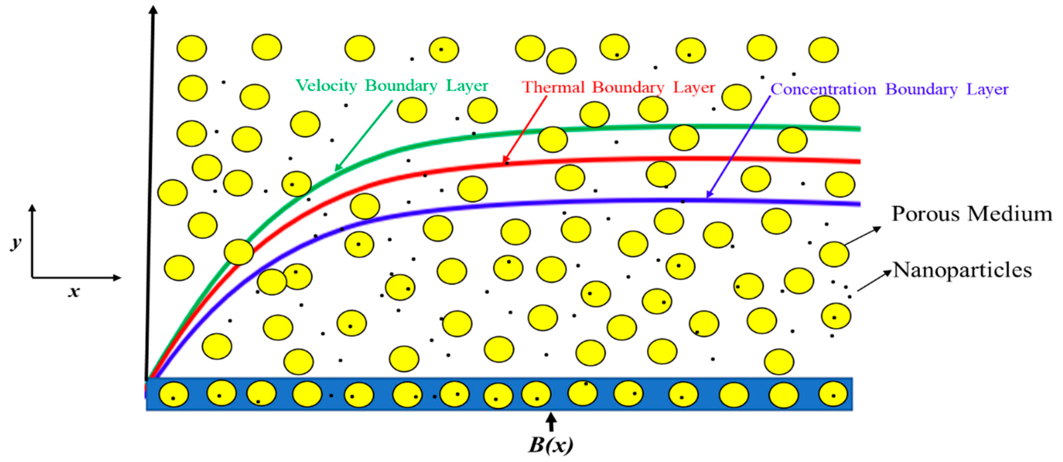
2. Mathematical Description of the Problem

We considered the steady incompressible two-dimensional flow of a Casson electrically conductive nanofluid over an exponentially shrinking surface in Extended Darcy Forchheimer porous medium along with the effects of viscous dissipations and slip conditions, as shown in Figure 1. According to Nakamura and Sawada [39], the rheological equation of the state for isotropic and incompressible flow of a Casson fluid are:

$${\tau }_{ij}=\{\begin{array}{c}\left({\mu }_B+\left(\frac{P_y}{\sqrt{2\pi }}\right)\right)2e_{ij},\pi >{\pi }_c\\ \left({\mu }_B+\left(\frac{P_y}{\sqrt{2{\pi }_c}}\right)\right)2e_{ij},\pi <{\pi }_c\end{array}$$

(1)

where ${\mu }_B$ denotes the plastic dynamic viscosity, $P_y$ denotes the yield stress of the fluid, $\pi$ denotes the product of deformation rate component, where π = $e_{ij}.e_{ij}$ is the (i, j)th deformation rate component and ${\pi }_c$ is a critical value of $\pi$, which is based on the non-Newtonian model. A Cartesian coordinate system is considered, where the x-axis is assumed along with a shrinking sheet and the y-axis is perpendicular to it. The uniform magnetic field of strength $B_0$ was applied normal to a shrinking sheet. The induced magnetic field was ignored due to the small value of the magnetic Reynolds number. According to these conditions, the governing equations for steady Casson nanofluid flow can be written as:

$$\frac{\partial u}{\partial x}+\frac{\partial v}{\partial y}=0$$

(2)

$$u\frac{\partial u}{\partial x}+v\frac{\partial u}{\partial y}=\vartheta \left(1+\frac{1}{\beta }\right)\frac{{\partial }^{2}u}{\partial y^2}-\frac{\vartheta \phi }{K}u-\frac{b}{\sqrt{K}}{u}^2-\frac{\sigma B^{2}u}{\rho }$$

(3)

$$u\frac{\partial T}{\partial x}+v\frac{\partial T}{\partial y}=\alpha \frac{{\partial }^{2}T}{\partial y^2}+{\tau }_1\left[D_B\frac{\partial C}{\partial y}\frac{\partial T}{\partial y}+\frac{D_T}{T_{\infty }}{\left(\frac{\partial T}{\partial y}\right)}^2\right]+\frac{\mu }{\rho c_p}\left(1+\frac{1}{\beta }\right){\left(\frac{\partial u}{\partial y}\right)}^2$$

(4)

$$u\frac{\partial C}{\partial x}+v\frac{\partial C}{\partial y}=D_B\frac{{\partial }^{2}C}{\partial y^2}+\frac{D_T}{T_{\infty }}\frac{{\partial }^{2}T}{\partial y^2}$$

(5)

The associated boundary conditions related to Equations (2)–(5) are:

$$\{\begin{array}{c}v=v_w,u=u_w+A\vartheta \left(1+\frac{1}{\beta }\right)\frac{\partial u}{\partial y},T=T_w\left(x\right)+D\frac{\partial T}{\partial y},C=C_w\left(x\right)+N\frac{\partial C}{\partial y}aty=0\\ u\to 0,T\to T_{\infty },C\to C_{\infty }asy\to \infty \end{array}$$

(6)

where u and v represent velocity components in the x- and the y-directions, respectively; $\rho ,\beta ,\vartheta ,\sigma ,\phi ,b,K,T,$ and $\alpha$ are the density of the fluid, Casson fluid parameter, kinematic viscosity, the electrical conductivity of fluid, porosity, the local inertia coefficient, porosity, permeability of the porous medium, fluid temperature, and the thermal diffusivity of the Casson nanofluid, respectively; and $B=B_0{e}^{\raisebox{1ex}{$x$}\!\left/ \!\raisebox{-1ex}{$2l$}\right.}$ is the magnetic field by the constant magnetic strength $B_0$. ${\tau }_1=\frac{{\left(\rho c\right)}_p}{{\left(\rho c\right)}_f}$ is the ratio between the effective heat capacity of the nanoparticle material and the capacity of the fluid; and $D_T$ are the coefficients of Brownian diffusion and thermophoretic diffusion, respectively; $T_w=T_{\infty }+T_0{e}^{\frac{x}{2\ell }}$ and $C_w=C_{\infty }+C_0{e}^{\frac{x}{2\ell }}$ are the temperature and concentration of the wall, respectively; where $T_{\infty }$ and $C_{\infty }$ are the ambient temperature and concentration, respectively. $v_w=-\sqrt{\frac{\vartheta a}{2l}}{e}^{\raisebox{1ex}{$x$}\!\left/ \!\raisebox{-1ex}{$2l$}\right.}S$, where S is the suction and blowing parameter, $u_w=-a{e}^{\raisebox{1ex}{$x$}\!\left/ \!\raisebox{-1ex}{$l$}\right.}$ is the shrinking velocity of surface, $A=A_1{e}^{\raisebox{1ex}{$-x$}\!\left/ \!\raisebox{-1ex}{$2l$}\right.}$ is the velocity slip factor, $D=D_1{e}^{\raisebox{1ex}{$-x$}\!\left/ \!\raisebox{-1ex}{$2l$}\right.}$ is the thermal slip factor, and $N=N_1{e}^{\raisebox{1ex}{$-x$}\!\left/ \!\raisebox{-1ex}{$2l$}\right.}$ is the concentration slip factor.

To obtain the similarity solutions, the following similarity transformations are used:

$$\psi =\sqrt{2\vartheta la}{e}^{\raisebox{1ex}{$x$}\!\left/ \!\raisebox{-1ex}{$2l$}\right.}f\left(\eta \right),\theta \left(\eta \right)=\frac{\left(T-T_{\infty }\right)}{\left(T_w-T_{\infty }\right)},\varnothing \left(\eta \right)=\frac{\left(C-C_{\infty }\right)}{\left(C_w-C_{\infty }\right)},\eta =y\sqrt{\frac{a}{2\vartheta l}}{e}^{\raisebox{1ex}{$x$}\!\left/ \!\raisebox{-1ex}{$2l$}\right.}$$

(7)

The stream function $\psi$ is written as a velocity component as:

$$u=\frac{\partial \psi }{\partial y},v=-\frac{\partial \psi }{\partial x}$$

(8)

The permeability of porous medium is taken as $K=2K_0{e}^{\raisebox{1ex}{$-x$}\!\left/ \!\raisebox{-1ex}{$l$}\right.}$. Note, the similarity transformation is mostly used to reduce the number of variables; the resultant equations are reduced to simple form. The similarity transformation is used to obtain the similarity solution. From a physical point of view, the meaning of similarity solutions is that “the velocity, temperature, and concentration profiles of the flow remain geometrically similar in each transversal section of the surface”. By applying Equations (7) and (8) into Equations (2)–(6), the continuity equation is satisfied and momentum, energy, and the concentration equations can be expressed as:

$$f^{‴}+\frac{\beta }{\left(1+\beta \right)}f{f}^{″}-\frac{\beta \left(2+F_S\right)}{\left(1+\beta \right)}{f}^{\prime 2}-\frac{\beta \left(K_1+M\right)}{\left(1+\beta \right)}{f}^{\prime }=0$$

(9)

$$\frac{1}{Pr}{\theta }^{″}+f{\theta }^{\prime }-f^{\prime }\theta +Nb{\varnothing }^{\prime }{\theta }^{\prime }+Nt{\left({\theta }^{\prime }\right)}^2+Ec.\left(1+\frac{1}{\beta }\right){\left(f^{″}\right)}^2=0$$

(10)

$${\varnothing }^{″}+Sc\left(f{\varnothing }^{\prime }-f^{\prime }\varnothing \right)+\frac{Nt}{Nb}{\theta }^{″}=0$$

(11)

along the boundary conditions

$$\begin{array}{c}f\left(0\right)=S,f^{\prime }\left(0\right)=-1+\delta \left(1+\frac{1}{\beta }\right)f^{″}\left(0\right),\\ \theta \left(0\right)=1+{\delta }_T\theta \prime \left(0\right),\varnothing \left(0\right)=1+{\delta }_C\varnothing \prime \left(0\right),\\ f^{\prime }\left(\eta \right)\to 0,\theta \left(\eta \right)\to 0,\varnothing \left(\eta \right)\to 0as\eta \to \infty \end{array}$$

(12)

where $M$ (range 0 to 0.5), $K_1$ (0–0.2), $F_S$ (range 0.05–1.15), $Pr$, (0.7–2.5), $N_b$, (0.05–0.5), $N_t$, (0–0.5), $Ec$, (0–0.7) and $Sc$ (0–1) denote the Hartmann number, permeability parameter, Forchheimer parameter, Prandtl number, Brownian motion parameter, thermophoresis parameter, Eckert number, and Schmidt number, respectively; $\delta$ (range 0–0.5), ${\delta }_T$ (0–0.5), and ${\delta }_C$ (0–0.5) are the velocity, thermal, and concentration slip parameters, respectively. The dimensionless quantities are defined as:

$$\{\begin{array}{c}M=\frac{2l\sigma {\left(B_0\right)}^2}{\rho a},K_1=\frac{l\vartheta }{a{K}_0},F_S=\frac{2lb}{\sqrt{K}},Pr=\frac{\vartheta }{\alpha },Sc=\frac{\vartheta }{D_B}\\ N_b=\frac{{\tau }_1{D}_B\left(C_w-C_{\infty }\right)}{\vartheta },N_t=\frac{{\tau }_1{D}_T\left(T_w-T_{\infty }\right)}{\vartheta T_{\infty }}\\ Ec=\frac{a^2}{C_p{T}_0},,\delta =A_1\sqrt{\frac{\vartheta a}{2l}},{\delta }_T=D_1\sqrt{\frac{a}{2\vartheta l}},{\delta }_C=N_1\sqrt{\frac{a}{2\vartheta l}}\end{array}$$

(13)

Physical quantities of interest include coefficient of skin friction, the local Nusselt number, and local Sherwood number, which are given by:

$$\begin{array}{c}{C}_f=\frac{{\left[\mu \left(1+\frac{1}{\beta }\right)\frac{\partial u}{\partial y}\right]}_{y=0}}{\rho a^2},N_u=\frac{-x{\left(\frac{\partial T}{\partial y}\right)}_{y=0}}{\left(T_w-T_{\infty }\right)},S_h=\frac{-x{\left(\frac{\partial C}{\partial y}\right)}_{y=0}}{\left(C_w-C_{\infty }\right)}\\ C_f{\left(R{e}_x\right)}^{\frac{1}{2}}=\left(1+\frac{1}{\beta }\right)f^{″}\left(0\right),N_u{\left(R{e}_x\right)}^{-\frac{1}{2}}=-{\theta }^{\prime }\left(0\right),S_h{\left(R{e}_x\right)}^{-\frac{1}{2}}=-{\varnothing }^{\prime }\left(0\right)\end{array}$$

(14)

3. Linear Stability Analysis

Recently, many authors [39,40,41] investigated multiple solutions for different types of fluids under various fluid flow conditions. From an experimental point of view, it is worth investigating if the solutions are physically reliable. Therefore, linear stability is required to check the reliability of the solutions. To perform stability analysis, the governing boundary layer in Equations (3)–(5) were reduced to the following unsteady form, as suggested by Merkin [43] and Yasin et al. [38]:

$$\frac{\partial u}{\partial t}+u\frac{\partial u}{\partial x}+v\frac{\partial u}{\partial y}=\vartheta \left(1+\frac{1}{\beta }\right)\frac{{\partial }^{2}u}{\partial y^2}-\frac{\vartheta \phi }{K}u-\frac{b}{\sqrt{K}}{u}^2-\frac{\sigma B^{2}u}{\rho }$$

(15)

$$\frac{\partial T}{\partial t}+u\frac{\partial T}{\partial x}+v\frac{\partial T}{\partial y}=\alpha \frac{{\partial }^{2}T}{\partial y^2}+\tau \left[D_B\frac{\partial C}{\partial y}\frac{\partial T}{\partial y}+\frac{D_T}{T_{\infty }}{\left(\frac{\partial T}{\partial y}\right)}^2\right]+\frac{\mu }{\rho c_p}\left(1+\frac{1}{\beta }\right){\left(\frac{\partial u}{\partial y}\right)}^2$$

(16)

$$\frac{\partial C}{\partial t}+u\frac{\partial C}{\partial x}+v\frac{\partial C}{\partial y}=D_B\frac{{\partial }^{2}C}{\partial y^2}+\frac{D_T}{T_{\infty }}\frac{{\partial }^{2}T}{\partial y^2}$$

(17)

where t denotes the time. A new similarity transformation is introduced:

$$\begin{array}{c}\psi =\sqrt{2\vartheta la}{e}^{\raisebox{1ex}{$x$}\!\left/ \!\raisebox{-1ex}{$2l$}\right.}f\left(\eta ,\tau \right),\theta \left(\eta ,\tau \right)=\raisebox{1ex}{$\left(T-T_{\infty }\right)$}\!\left/ \!\raisebox{-1ex}{$\left(T_w-T_{\infty }\right)$}\right.\\ \varnothing \left(\eta ,\tau \right)=\raisebox{1ex}{$\left(C-C_{\infty }\right)$}\!\left/ \!\raisebox{-1ex}{$\left(C_w-C_{\infty }\right)$}\right.,\eta =y\sqrt{\frac{a}{2\vartheta l}}{e}^{\raisebox{1ex}{$x$}\!\left/ \!\raisebox{-1ex}{$2l$}\right.},\tau =\frac{a}{2l}{e}^{\raisebox{1ex}{$x$}\!\left/ \!\raisebox{-1ex}{$l$}\right.}.t\end{array}$$

(18)

Using Equation (18), Equations (15)–(17) can be written as:

$$\left(1+\frac{1}{\beta }\right)\frac{{\partial }^{3}f\left(\eta ,\tau \right)}{\partial {\eta }^3}+f\left(\eta ,\tau \right)\frac{{\partial }^{2}f\left(\eta ,\tau \right)}{\partial {\eta }^2}-\left(2+F_S\right){\left(\frac{\partial f\left(\eta ,\tau \right)}{\partial \eta }\right)}^2-\left(K_1+M\right)\frac{\partial f\left(\eta ,\tau \right)}{\partial \eta }-\frac{{\partial }^{2}f\left(\eta ,\tau \right)}{\partial \tau \partial \eta }=0$$

(19)

$$\begin{array}{r}\frac{{\partial }^2\theta \left(\eta ,\tau \right)}{\partial {\eta }^2}+Pr(f\left(\eta ,\tau \right)\frac{\partial \theta \left(\eta ,\tau \right)}{\partial \eta }-\frac{\partial f\left(\eta ,\tau \right)}{\partial \eta }\theta \left(\eta ,\tau \right)+Nb\frac{\partial \varnothing \left(\eta ,\tau \right)}{\partial \eta }\frac{\partial \theta \left(\eta ,\tau \right)}{\partial \eta }\\ +Nt{\left(\frac{\partial \theta \left(\eta ,\tau \right)}{\partial \eta }\right)}^2+Ec.\left(1+\frac{1}{\beta }\right){\left(\frac{{\partial }^{2}f\left(\eta ,\tau \right)}{\partial {\eta }^2}\right)}^2-\frac{\partial \theta \left(\eta ,\tau \right)}{\partial \tau })=0\end{array}$$

(20)

$$\frac{{\partial }^2\varnothing \left(\eta ,\tau \right)}{\partial {\eta }^2}+Sc\left(f\left(\eta ,\tau \right)\frac{\partial \varnothing \left(\eta ,\tau \right)}{\partial \eta }-\frac{\partial f\left(\eta ,\tau \right)}{\partial \eta }\varnothing \left(\eta ,\tau \right)\right)+\frac{Nt}{Nb}\frac{{\partial }^2\theta \left(\eta ,\tau \right)}{\partial {\eta }^2}-\frac{\partial \varnothing \left(\eta ,\tau \right)}{\partial \tau }=0$$

(21)

along with new boundary conditions:

$$\begin{array}{cc}\hfill f\left(0,\tau \right)=& S,\frac{\partial f\left(0,\tau \right)}{\partial \eta }=-1+\delta \left(1+\frac{1}{\beta }\right)\frac{{\partial }^{2}f\left(0,\tau \right)}{\partial {\eta }^2},\theta \left(0,\tau \right)=1+{\delta }_T\frac{\partial \theta \left(0,\tau \right)}{\partial \eta },\varnothing \left(0,\tau \right)\hfill \\ \hfill =& 1+{\delta }_C\frac{\partial \varnothing \left(0,\tau \right)}{\partial \eta }\hfill \\ & \frac{\partial f\left(\eta ,\tau \right)}{\partial \eta }\to 0,\theta \left(\eta ,\tau \right)\to 0,\varnothing \left(\eta ,\tau \right)\to 0as\eta \to \infty \hfill \end{array}$$

(22)

To check the stability of the steady flow solutions, where $f\left(\eta \right)=f_0\left(\eta \right),\theta \left(\eta \right)={\theta }_0\left(\eta \right)$ and satisfy the boundary value problem in Equations (9)–(12), we write:

$$\begin{array}{c}f\left(\eta ,\tau \right)=f_0\left(\eta \right)+e^{-\epsilon \tau }F\left(\eta ,\tau \right)\\ \theta \left(\eta ,\tau \right)={\theta }_0\left(\eta \right)+e^{-\epsilon \tau }G\left(\eta ,\tau \right)\\ \varnothing \left(\eta ,\tau \right)={\varnothing }_0\left(\eta \right)+e^{-\epsilon \tau }H\left(\eta ,\tau \right)\end{array}$$

(23)

where $F\left(\eta \right)$, $G\left(\eta \right)$, and $H\left(\eta \right)$ are small relative values of $f_0\left(\eta \right)$, ${\theta }_0\left(\eta \right),$ and ${\varnothing }_0\left(\eta \right)$ respectively; and $\epsilon$ is the unknown eigenvalues. When we solve the eigenvalue problem in Equations (19)–(22), we have an infinite set of eigenvalues. From that set, we chose the smallest eigenvalue. If the smallest eigenvalue ($\epsilon$) is negative, the flow is unstable and the disturbances grow, which is physically not possible. If the smallest eigenvalue is positive, it suggests that the solution is stable and physically reliable. Applying the relations in Equation (23) into Equations (19)–(22), the following equations are obtained:

$$\left(1+\frac{1}{\beta }\right)F_0^{‴}+f_0{F}_0^{″}+F_0{f}_0^{″}-2\left(2+F_S\right)f_0^{\prime }{F}_0^{\prime }-\left(K_1+M\right)F_0^{\prime }+\epsilon F_0^{\prime }=0$$

(24)

$$\begin{array}{c}\frac{1}{Pr}{G}_0^{″}+f_0{G}_0^{\prime }+F_0{\theta }_0^{\prime }-f_0^{\prime }{G}_0-F_0^{\prime }{\theta }_0+Nb{\varnothing }_0^{\prime }{G}_0^{\prime }+Nb{H}_0^{\prime }{\theta }_0^{\prime }+2Nt{\theta }_0^{\prime }{G}_0^{\prime }\\ +2Ec.\left(1+\frac{1}{\beta }\right)f_0^{″}{F}_0^{″}+\epsilon G_0=0\end{array}$$

(25)

$$H_0^{″}+Sc\left\{\left(f_0{\varnothing }_0^{\prime }+F_0{H}_0^{\prime }\right)-\left(f_0^{\prime }{H}_0+F_0^{\prime }{\varnothing }_0\right)\right\}+\frac{Nt}{Nb}{G}_0^{″}+Sc\epsilon H_0=0$$

(26)

subject to boundary condition:

$$\begin{array}{c}{F}_0\left(0\right)=0,F_0^{\prime }\left(0\right)=\delta \left(1+\frac{1}{\beta }\right)F_0^{″}\left(0\right),G_0\left(0\right)={\delta }_T{G}_0^{\prime }\left(0\right),H_0\left(0\right)={\delta }_C{H}_0^{\prime }\left(0\right),\\ F_0^{\prime }\left(\eta \right)\to 0,G_0\left(\eta \right)\to 0,H_0\left(\eta \right)\to 0,as\eta \to \infty \end{array}$$

(27)

According to Haris et al. [41], to determine the stability of Equations (24)–(27), we need to relax one boundary condition on $F_0^{\prime }\left(\eta \right),G_0\left(\eta \right)$, and $H_0\left(\eta \right)$. We relaxed $F_0^{\prime }\left(\eta \right)\to 0\mathrm{as}\eta \to \infty$ into $F_0^{″}\left(0\right)=1$ in this problem. We fixed the all parameters to: $\beta =1.5,F_S=0.2,K_1=0.1,Pr=1,Nt=0.15,Nb=0.2,Ec=0.1,Sc=1,\delta =0.1,\mathrm{and}{\delta }_C=0.1$, and varied the values of M and ${\delta }_T$.

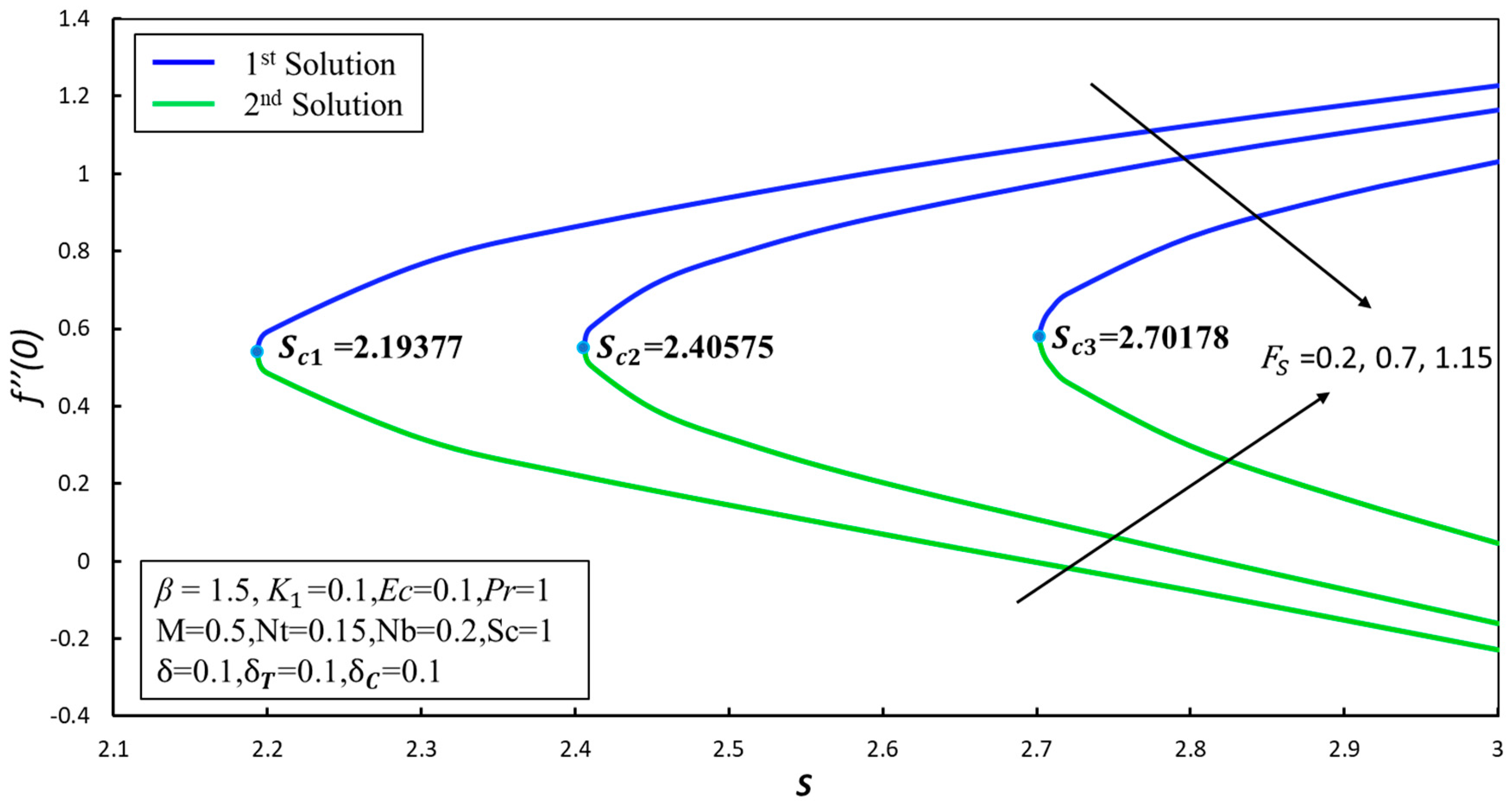
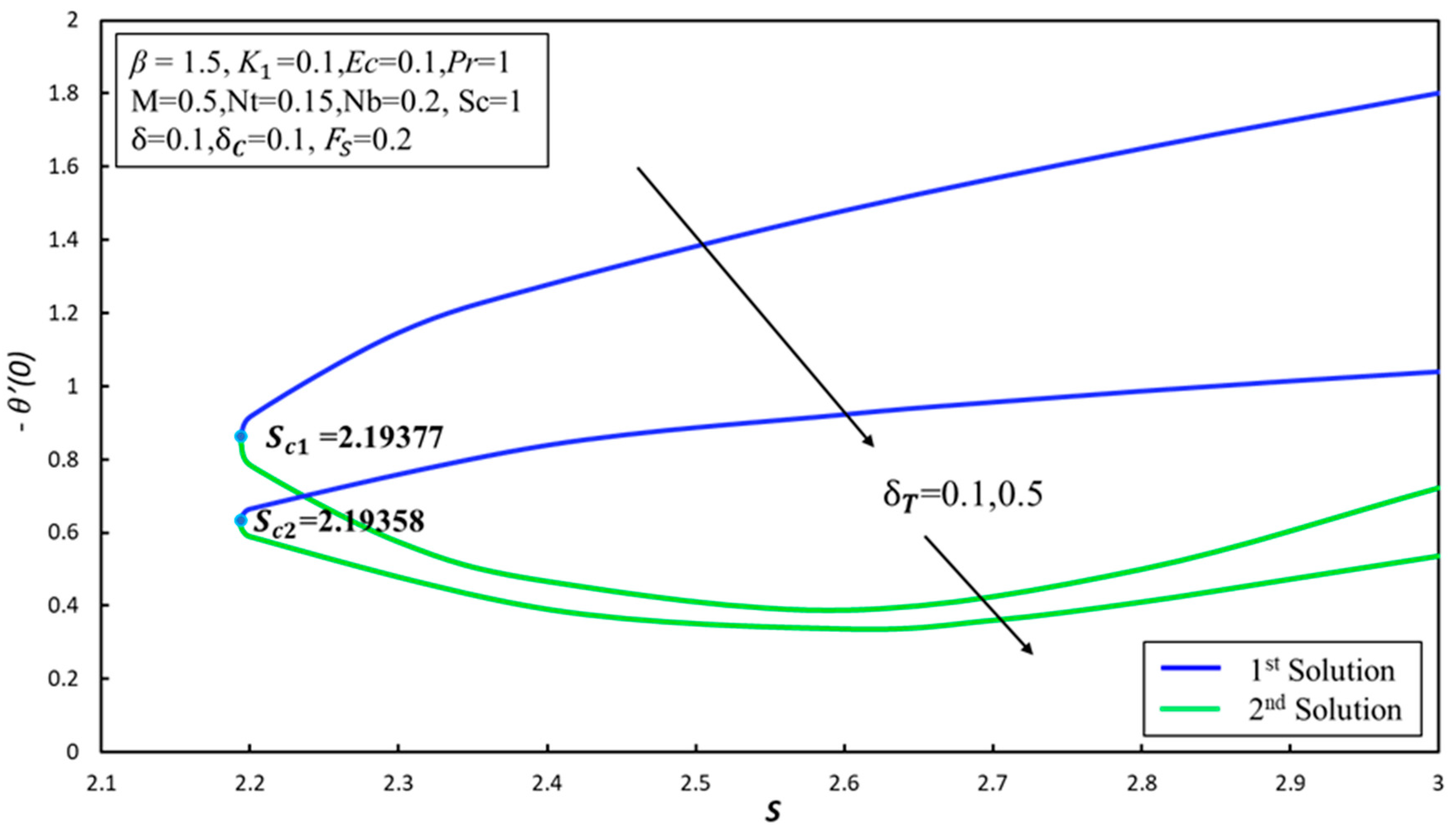
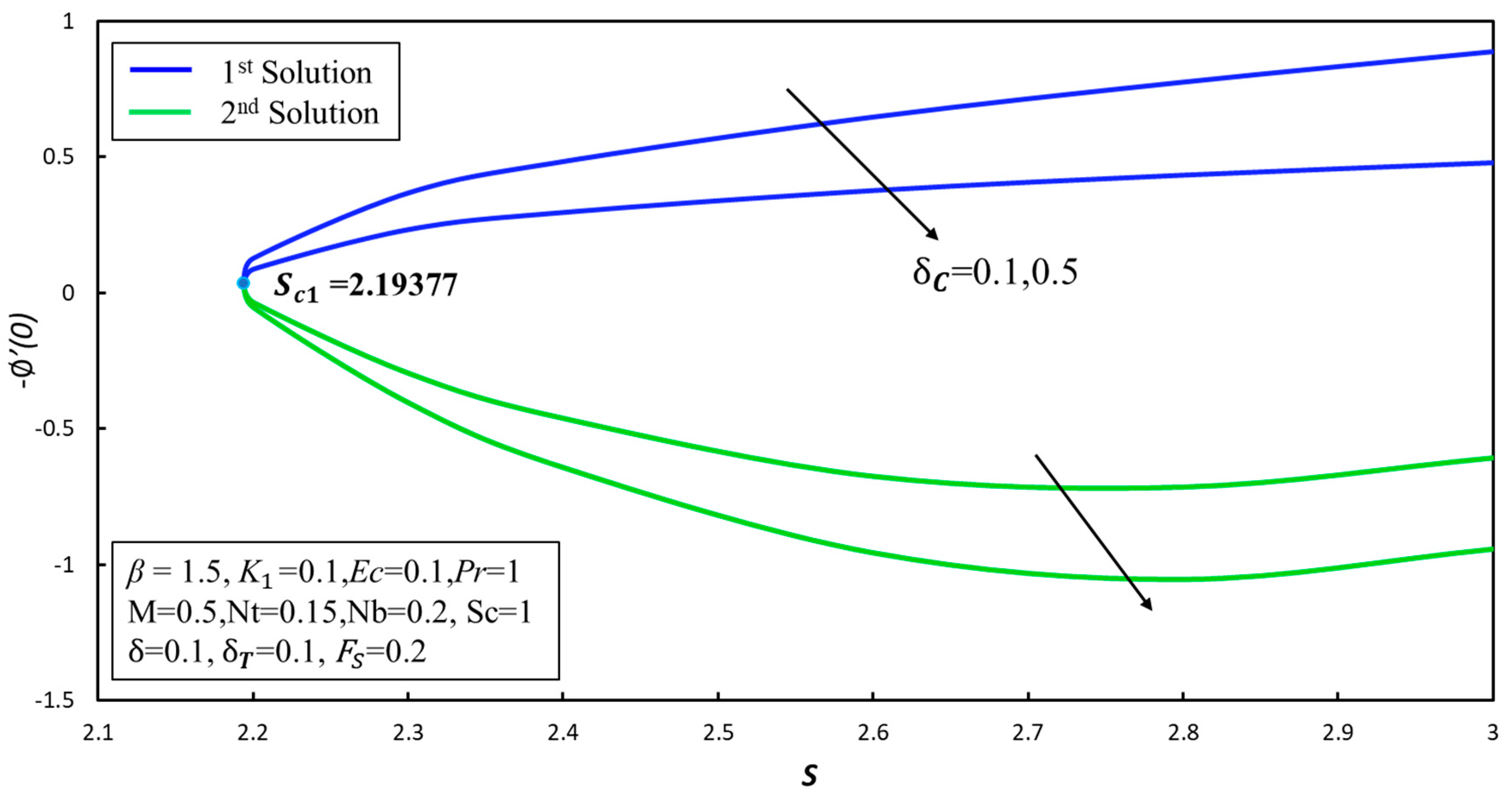
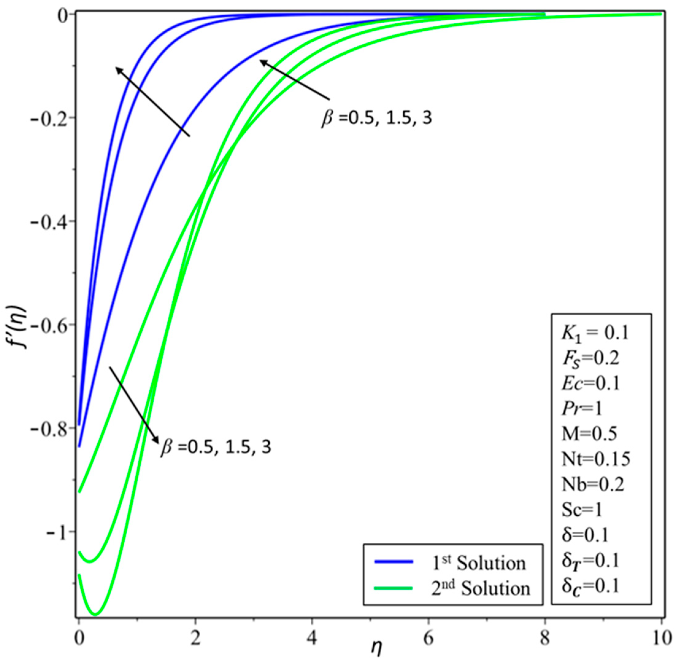
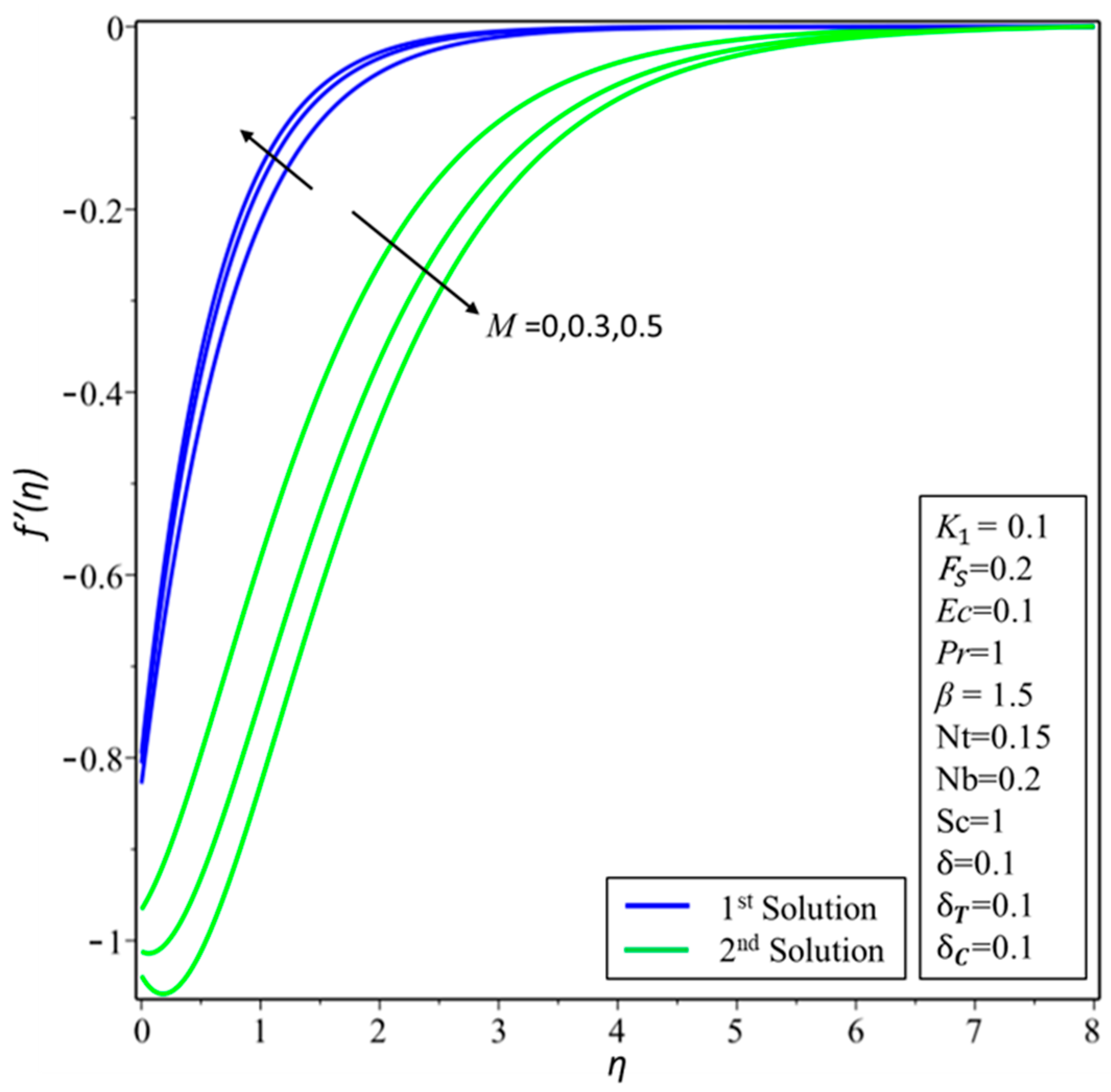
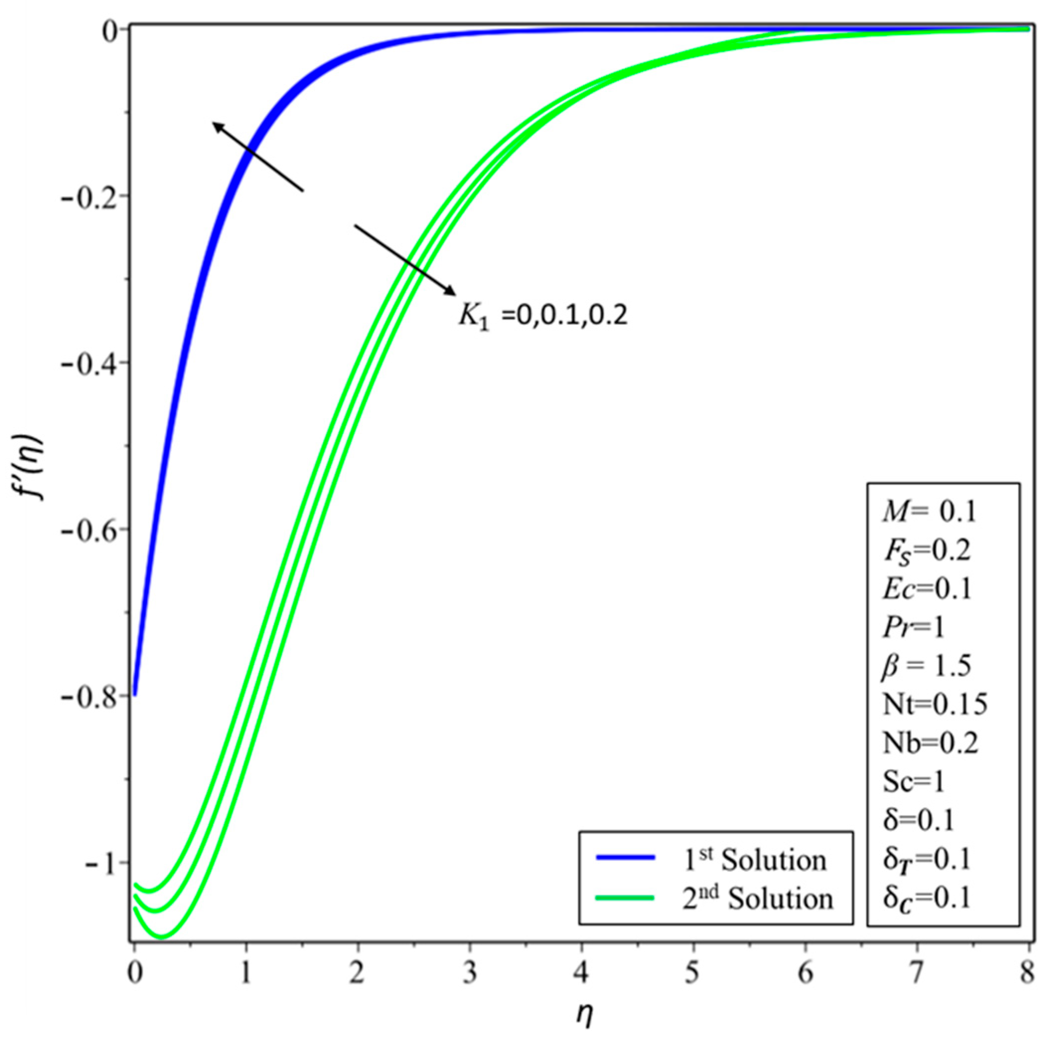
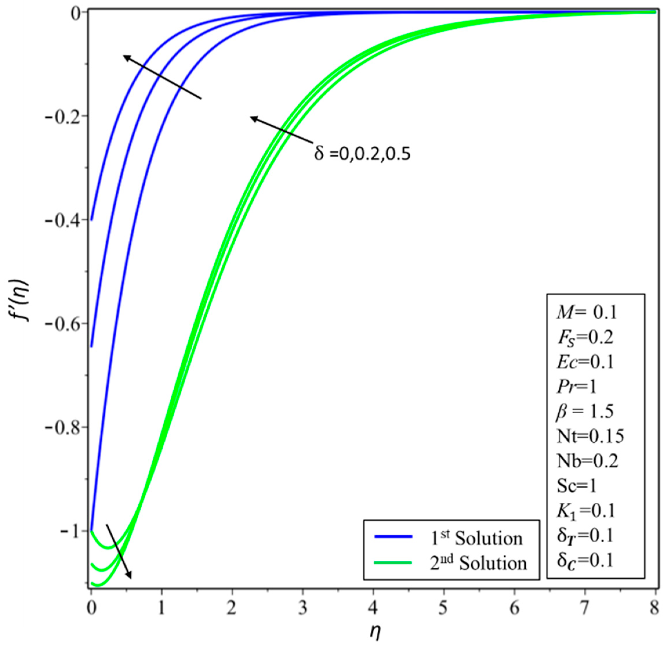
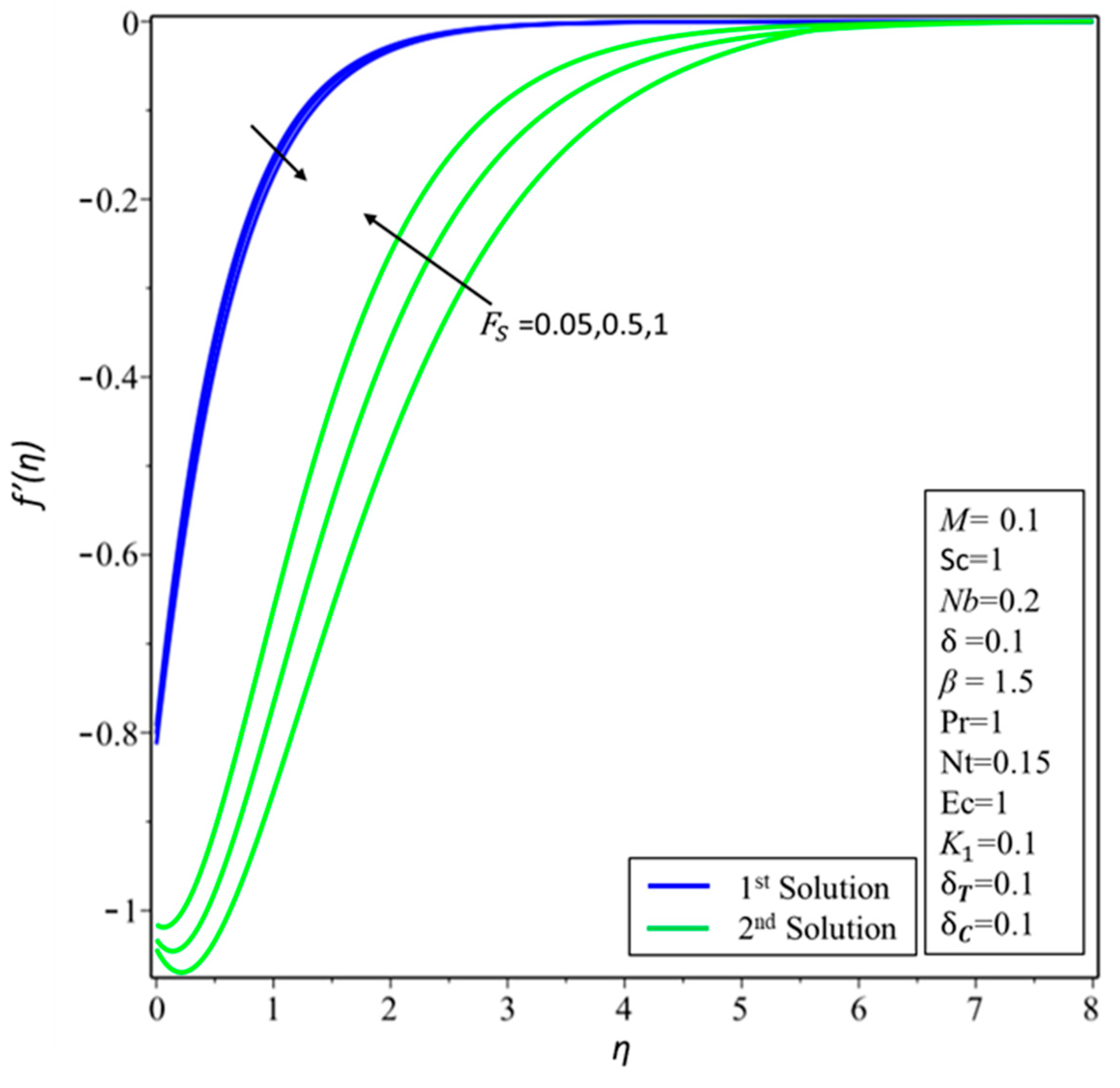
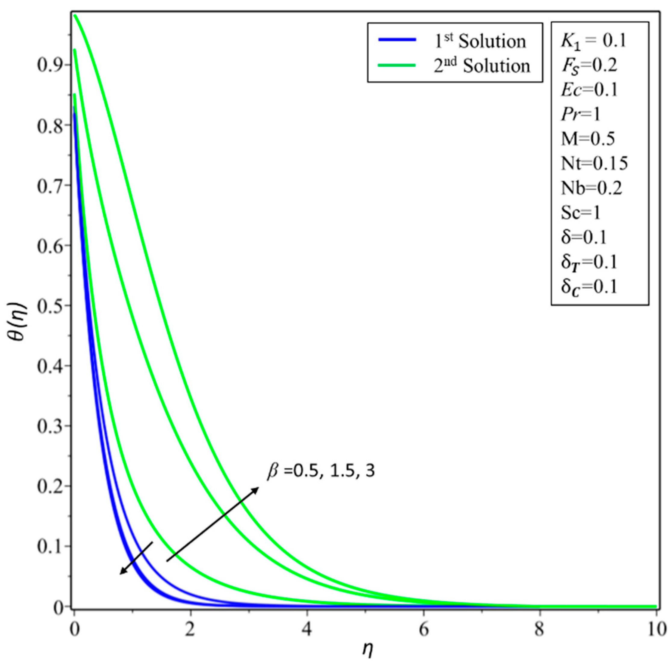
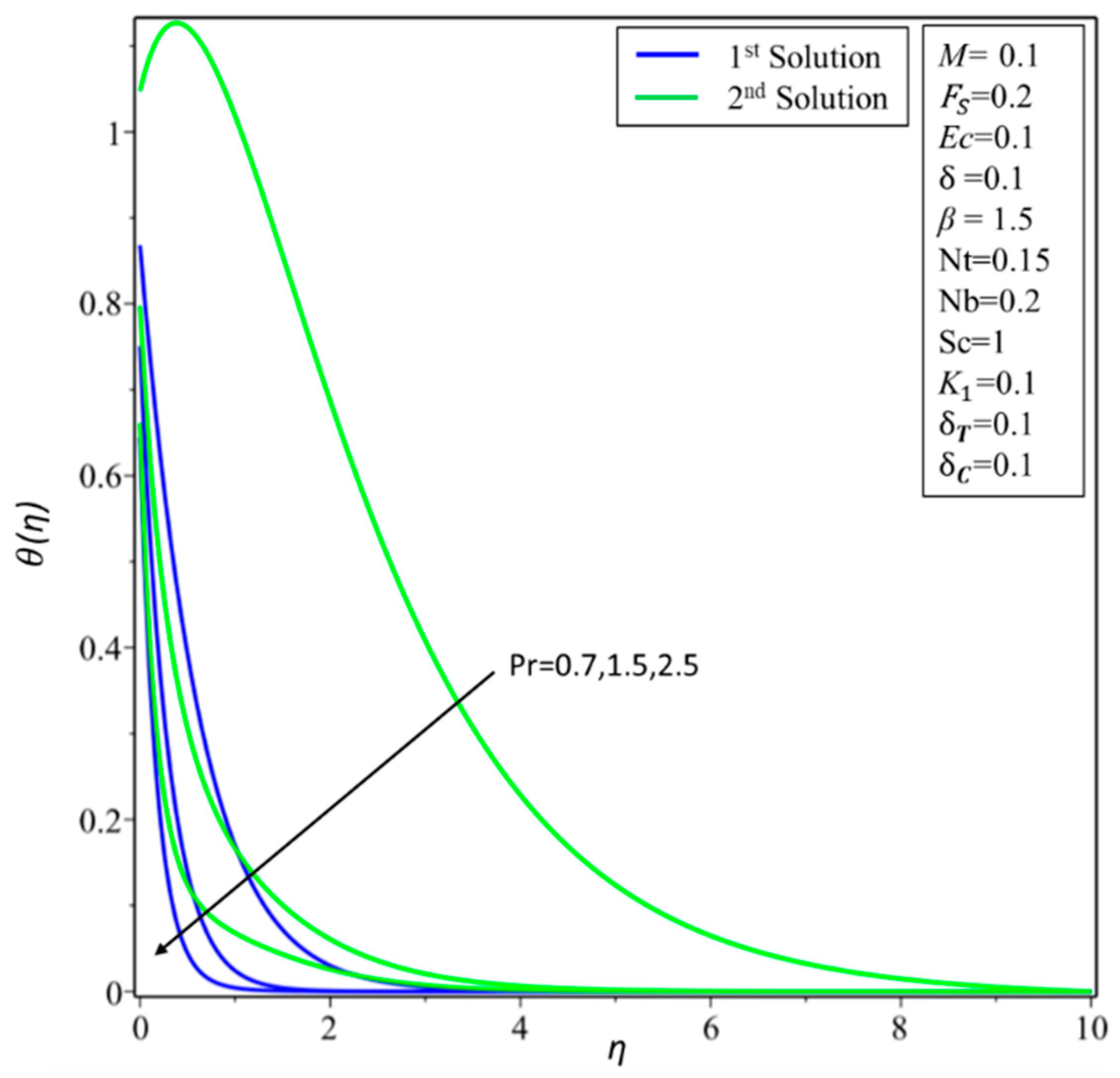
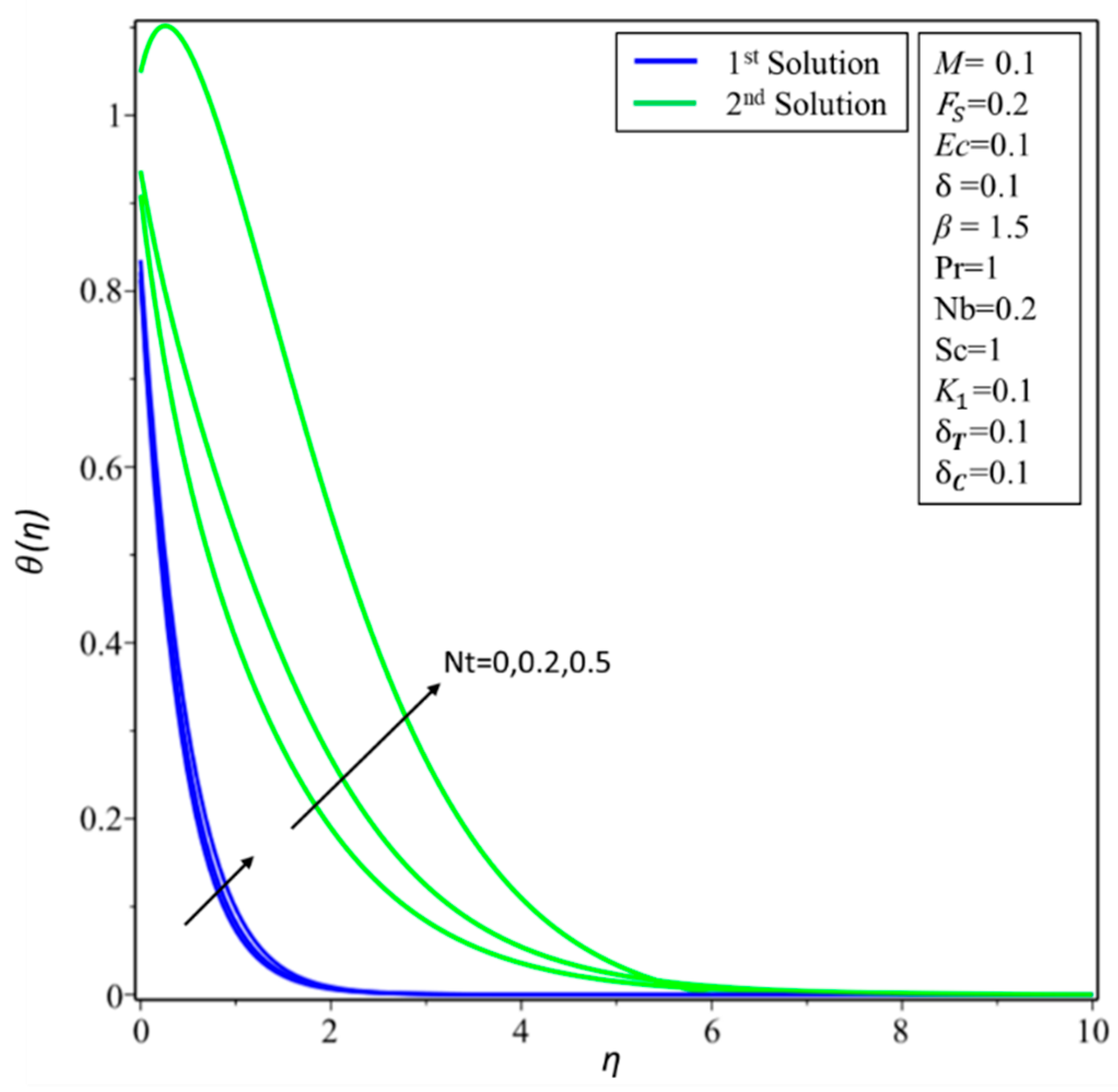
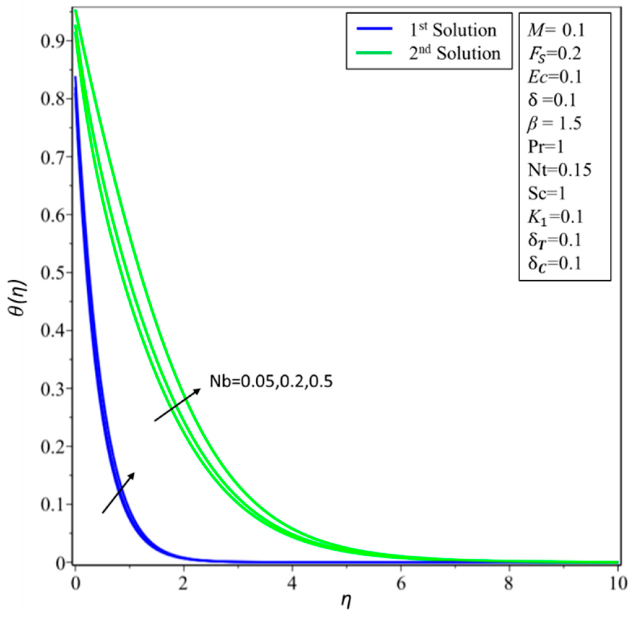
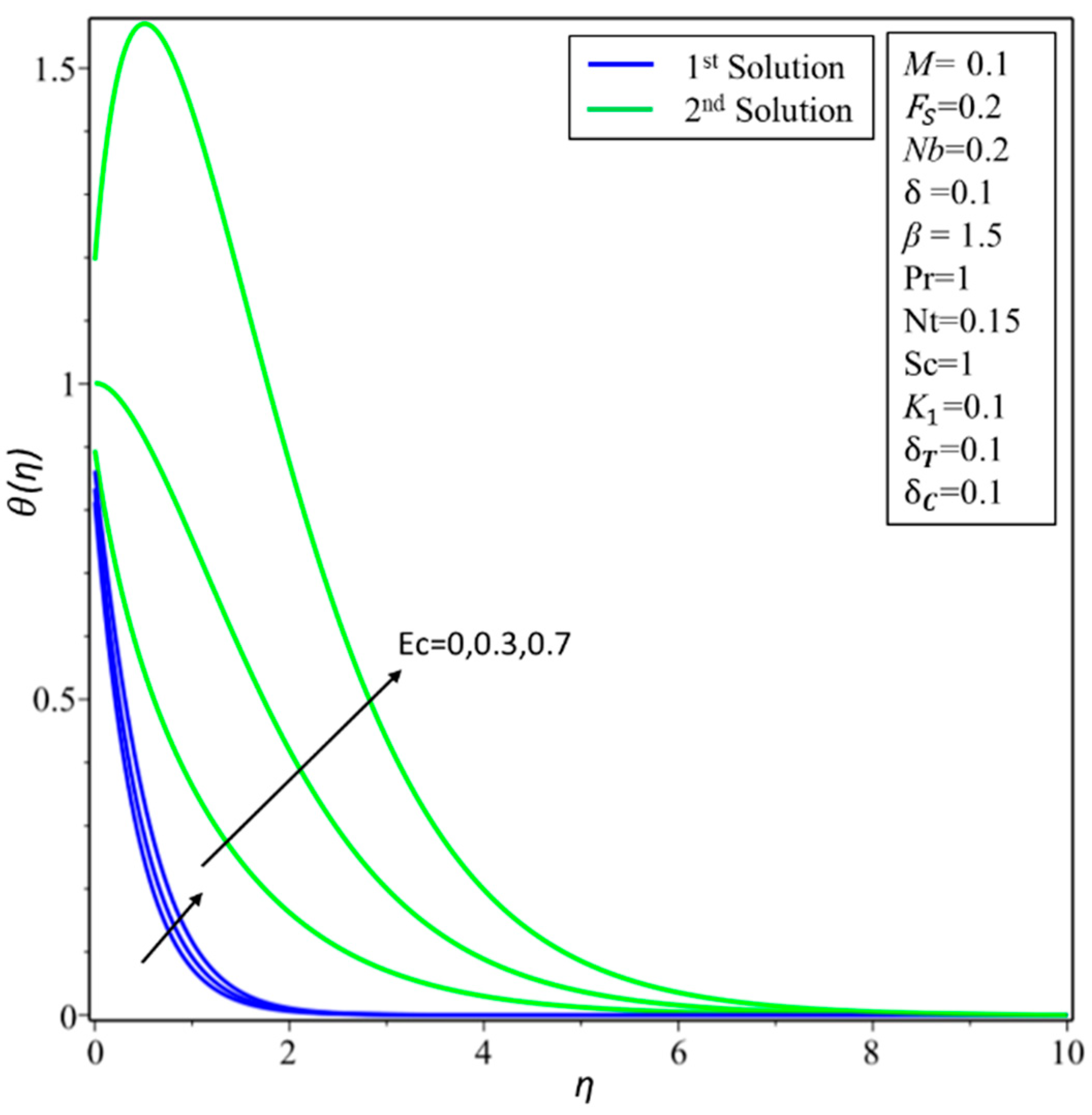
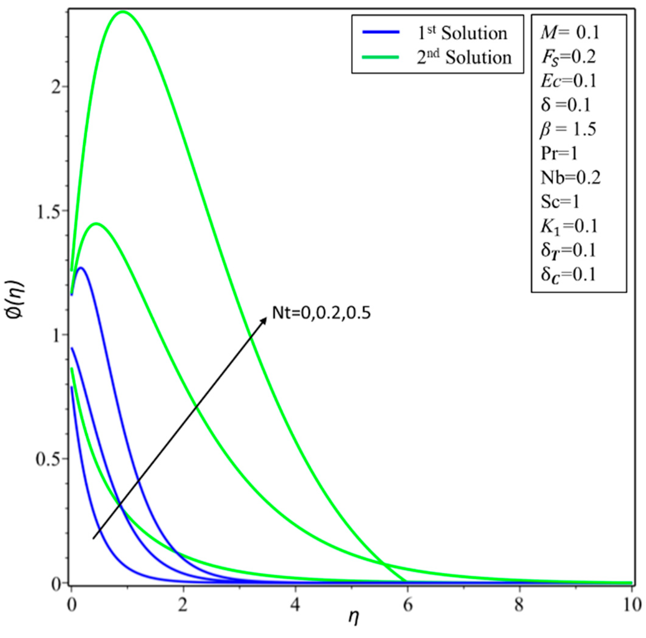
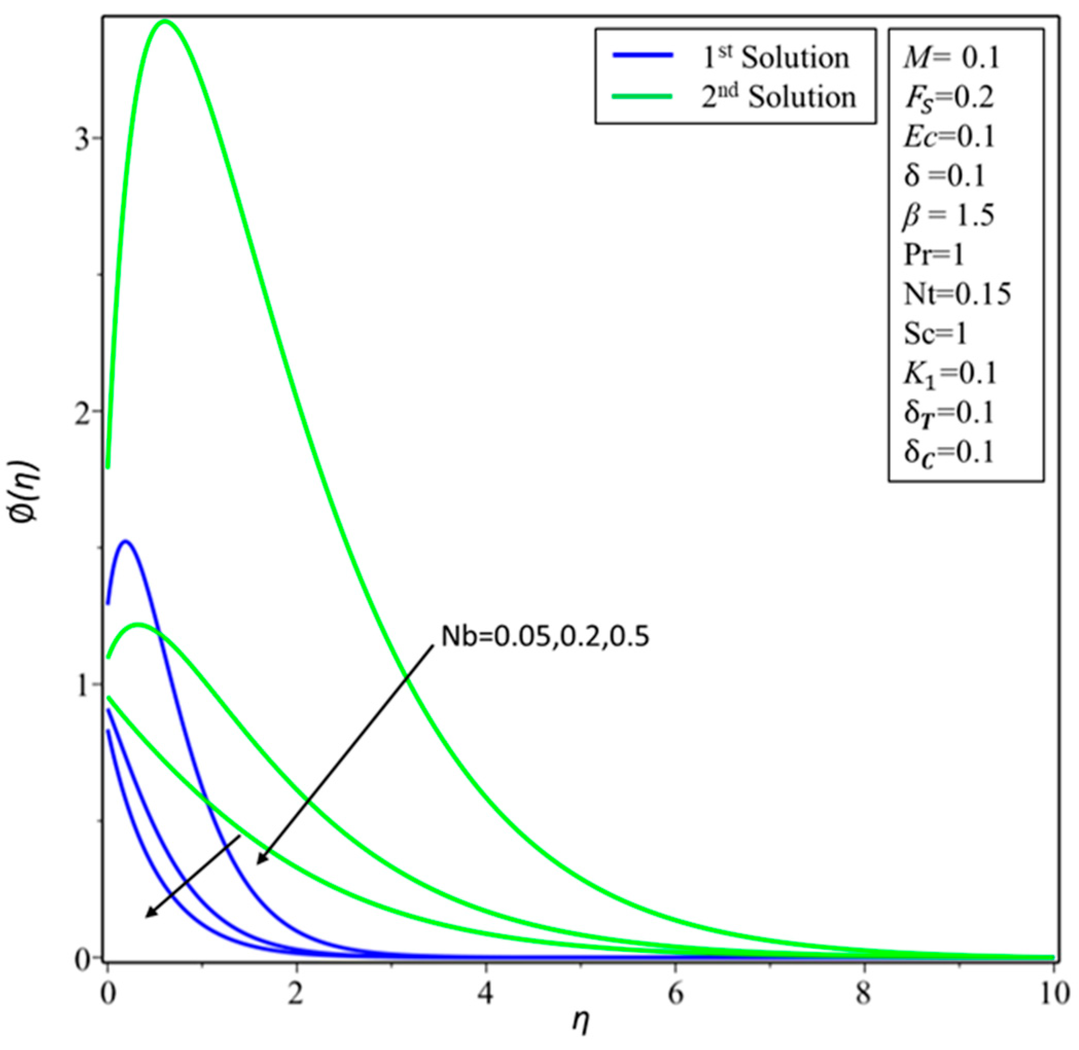
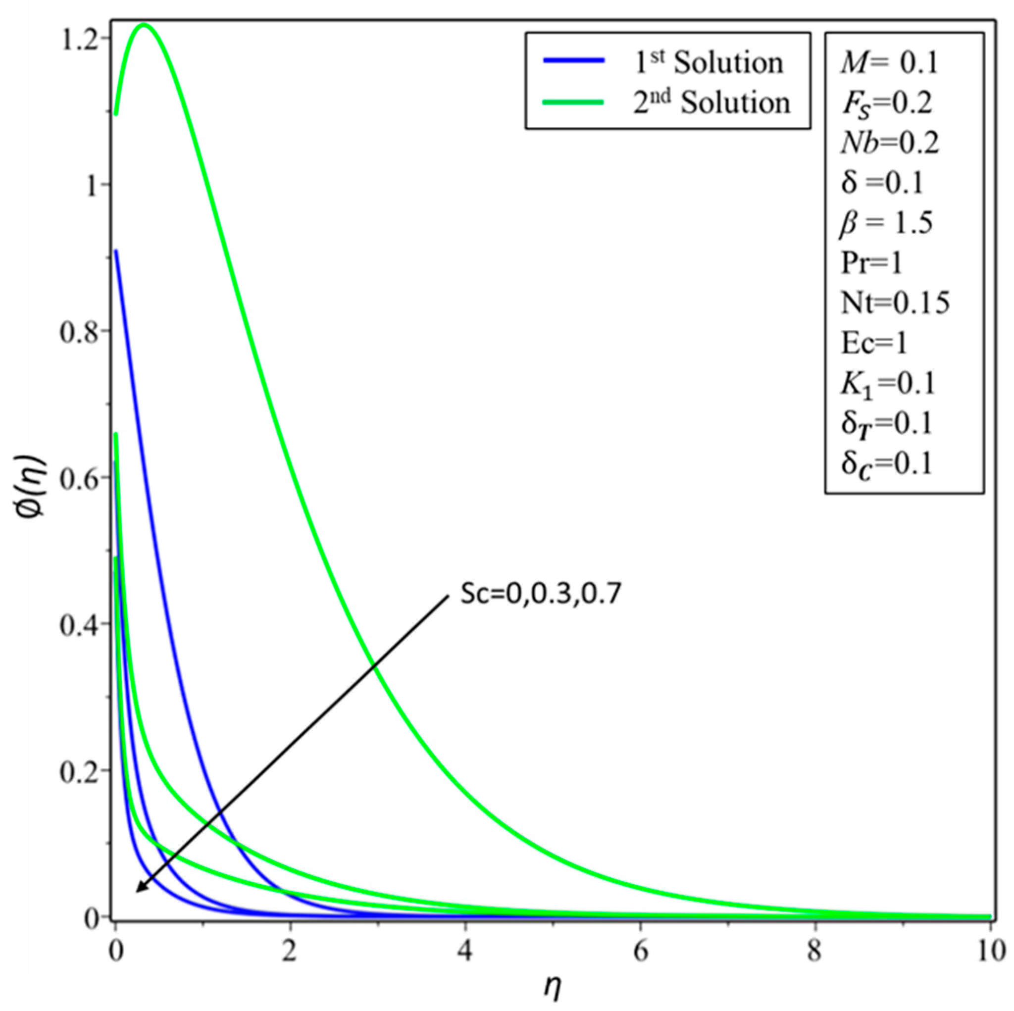
4. Result and Discussion

With the help of the shooting method, the transformed ordinary differential equations (BVPs) in Equations (9)–(11) along with the boundary conditions in Equation (12) were converted to initial value problems (IVPs). Equations of IVPs were solved via the Runge Kutta (RK) method. Another method, the three-stage Lobatto IIIa formula, was developed in bvp4c with the help of finite difference code. Later, stability analysis was conducted using the bvp4c solver function. According to Rehman et al. [36], “this collocation formula and the collocation polynomial provides a C¹ continuous solution that is fourth-order accurate uniformly in [a,b]. Mesh selection and error control are based on the residual of the continuous solution”. The impacts of various physical parameters, such as Forchheimer parameter, thermal slip parameter, Casson parameter, magnetic parameter, permeability parameter, Prandtl number, Brownian motion, and thermophoresis parameter, on the flow and heat transfer characteristics were explored. Figure 1 shows the physical model of the problem.

Figure 2 illustrates the existence of multiple solutions for the variation of suction parameter $S$ for three different values of the Forchheimmer parameter $F_S$. For all three values of the Forchheimmer parameter $F_S=0.2,0.7,1.15,$ there were critical points $S_{ci},i=1,2,3$, where multiple solutions exist. From a mathematical point of view, we know that the second solution cannot be produced experimentally, but the second solution is a part of the solution to the system of differential equations and therefore should be considered. Overall, we focused on the investigation of the occurrence of multiple solutions for the considered problem. From this profile, we concluded that there are only dual solutions if suction parameter $S$ satisfies this relation $S\ge S_{ci},i=1,2,3$. For the case of the first solution, the skin friction coefficient decreases strictly monotonically as the Forchheimer parameter $F_S$ increases. However, the opposite trend was observed for the second solution. Figure 3 depicts the occurrence of multiple solutions against the values of suction parameter $S$ for two values of thermal slip parameter ${\delta }_T$ on heat transfer rate $-\theta \prime \left(0\right)$. Multiple solutions exist for the variation in the thermal slip parameter ${\delta }_T=0.1,0.5$ only when the suction parameter $S\ge S_{c1}=2.19377$ and $S\ge S_{c2}=2.19358$. The heat transfer coefficient declines gradually for the variation in the thermal slip parameter ${\delta }_T$ against the values of suction parameter $S$. The occurrence of multiple solutions for the values of mass slip parameter ${\delta }_C$ against suction parameter can be seen in the concentration profile in Figure 4. From this profile, the critical point where multiple solutions exist is the same for the two different values of mass slip parameter ${\delta }_C$. The influence of Casson parameter $\beta$ on velocity profile $f\prime \left(\eta \right)$ for the variation in different physical parameters is shown in Figure 5. From this profile, the velocity profile and its thickness of boundary layer increase with increasing values of the Casson parameter for the first solution. However, the momentum boundary layer decreases for $0\le \eta <3$, due to the increase in a $\beta$ plastic dynamic, and the viscosity increased, causing resistance to the fluid motion. The opposite behavior was observed for the second solution.

The effect of the magnetic parameter $M$ on velocity profile is shown in Figure 6. The thickness of the boundary layer and the velocity of the nanofluid flow are enhanced for the first solution and reduced for the second solution by increasing the strength of the magnetic parameter. Physically, the thickness of boundary layer decreases by increasing the values of the magnetic parameter for the second solution because the fluid particle motion diffuses quickly into the neighboring fluid layers as the values of $M$ increase. Figure 7, Figure 8 and Figure 9 depict the effect of permeability parameter $K_1$, velocity slip parameter, and Forchheimmer parameter $F_S$ on the velocity profile for fixed values of various physical parameters. These profiles show that the hydrodynamic boundary layer increases in the first solution and decreases in the second solution by increasing the strength of the porosity. However the opposite trend was observed by increasing the Forchheimmer parameter $F_S.$ With increasing the velocity slip parameter $\mathsf{\delta }$, the velocity profile for both cases (first and second solutions) increases gradually. Figure 10 depicts the effects of the Casson parameter on temperature profile. The temperature and boundary layer thickness of the nanofluid flow decrease for the first solution and increase for the second solution. We concluded that, according to the physical point of view, due to an increase in elasticity, stress parameter thickening of the thermal boundary layer occurred. The Prandtl number $Pr$ effects on the temperature profile are exhibited in Figure 11. The temperature of the Casson nanofluid decreases with increasing $Pr$ and the thermal boundary layer thickness decreases. The Prandtl number can be defined as “the ratio of momentum diffusivity to thermal diffusivity”, which means a Casson nanofluid with a higher Prandtl number decreases thermal conductivity, which causes the reduction in the thermal boundary layer thickness.

Due to the increase in the thermophoresis parameter, the temperature profile and the thermal boundary layer of the nanofluid for the first and second solutions increase gradually (Figure 12). With the increase in thermophoresis parameter $N_t$ thermophoresis force increased, which helped nanoparticles to travel from hot to cold areas. Subsequently, the temperature of the nanofluid increased. Figure 13 shows the effects of the Brownian motion parameter $N_b$ on the temperature profile. This profile shows that temperature increased due to the increase in the Brownian motion parameter; therefore, thermal boundary layer thickness increased. Temperature profile increases as Eckert number increases; therefore, the thermal boundary layer increases gradually because an expansion in dissipation enhances the thermal conductivity of the flow, which upgrades the thermal boundary layers (Figure 14). The impact of thermophoresis parameter $N_t$ on the nanoparticle volume fraction $\phi \left(\eta \right)$ is depicted in Figure 15. The profile of the nanoparticle volume fraction increases with increasing values of the thermophoresis parameter $N_t$. Figure 16 presents the effects of the Brownian motion parameter $N_b$ on the nanoparticle volume fraction. This profile shows that the nanoparticle volume boundary layer thickness decreases as $N_b$ increases gradually. Figure 17 shows the effects of Schmidt number on concentration profile. Concentration profiles decrease as Sc increases. The comparison of the numerical results of our problem drawn from bvp4c and the shooting method is outlined in

Table 1. Comparison between bvp4c method and the shooting method for different values of $K_1$ and M when $\beta =1.5,F_S=0.2,Pr=1,Nt=0.15,Nb=0.2,Ec=0.1,Sc=1,\delta =0.1,{\delta }_T=0.1,\mathrm{and}{\delta }_C=0.1$.

M	${\mathit{K}}_1$		${\mathit{f}}^{″}\left(0\right)$
		bvp4c Method	Shooting Method
0.5	0.1	1.636957	1.636908
	0.2	1.651884	1.651959
	0.3	1.666407	1.666527
0	0.1	1.552846	1.552775
1		1.707631	1.707671
1.5		1.769173	1.769238

; the results from both methods showed an excellent agreement. The smallest eigenvalue $\epsilon$ for some values of $M$ and ${\delta }_T$ are shown in

Table 2. Smallest eigenvalues for different values of M and ${\delta }_T$.

M	${\mathit{\delta }}_{\mathit{T}}$		${\mathit{\epsilon }}_1$
		First Solution	Second Solution
0.5	0	0.87456	−1.04592
	0.1	0.73948	−1.00248
0.7	0	0.94310	−1.294601
	0.1	0.79092	−1.12253

. These values show that all values of $\epsilon$ are positive for the first solution and negative for the second solution. Therefore, we concluded that the first solution is stable while the second solution is unstable.

5. Conclusions

Two-dimensional MHD flow of a Casson nanofluid over a shrinking surface in an Extended Darcy Forchheimer porous medium with the effects of viscous dissipation, velocity, thermal, and concentration slip were examined numerically in this study. The governing boundary layer equations were converted into ordinary differential equations before solving them using the shooting method with the Runge Kutta method. The numerical results showed the existence of dual solutions. To determine which solutions were stable and unstable, stability analysis was conducted. The values of the smallest eigenvalues indicated that only first solution was stable. We found ranges of dual solutions, solutions that depended on a suction parameter, and no solution. Notably, as the Forchheimmer parameter $F_S$ increased, strong mass suction was required to obtain solutions. We found that the velocity profile is indirectly proportional to the velocity slip parameter in the first solution, and that the hydrodynamic boundary layer increases in the first solution and decreases in the second solution by increasing the strength of the porosity.

References

1. Nield, D.A.; Bejan, A. Convection in Porous Media; Springer: New York, NY, USA, 2006; Volume 3. [Google Scholar]
2. Muskat, M. The Flow of Homogeneous Fluids through Porous Media. No. 532.5 M88. 1946. Available online: https://catalog.hathitrust.org/Record/009073808 (accessed on 30 December 2018).
3. Bakar, S.A.; Arifin, N.M.; Nazar, R.; Ali, F.M.; Pop, I. Forced convection boundary layer stagnation-point flow in Darcy-Forchheimer porous medium past a shrinking sheet. Front. Heat Mass Transf. 2016, 7, 38. [Google Scholar]
4. Hayat, T.; Muhammad, T.; Al-Mezal, S.; Liao, S.J. Darcy-Forchheimer flow with variable thermal conductivity and Cattaneo-Christov heat flux. Int. J. Numer. Methods Heat Fluid Flow 2016, 26, 2355–2369. [Google Scholar] [CrossRef]
5. Muhammad, T.; Alsaedi, A.; Shehzad, S.A.; Hayat, T. A revised model for Darcy-Forchheimer flow of Maxwell nanofluid subject to convective boundary condition. Chin. J. Phys. 2017, 55, 963–976. [Google Scholar] [CrossRef]
6. Hayat, T.; Saif, R.S.; Ellahi, R.; Muhammad, T.; Alsaedi, A. Simultaneous effects of melting heat and internal heat generation in stagnation point flow of Jeffrey fluid towards a nonlinear stretching surface with variable thickness. Int. J. Therm. Sci. 2018, 132, 344–354. [Google Scholar] [CrossRef]
7. Alshomrani, A.S.; Ullah, M.Z. Effects of homogeneous-heterogeneous reactions and convective condition in Darcy-Forchheimer flow of carbon nanotubes. J. Heat Transf. 2019, 141, 012405. [Google Scholar] [CrossRef]
8. Hayat, T.; Saif, R.S.; Ellahi, R.; Muhammad, T.; Ahmad, B. Numerical study for Darcy-Forchheimer flow due to a curved stretching surface with Cattaneo-Christov heat flux and homogeneous-heterogeneous reactions. Results Phys. 2017, 7, 2886–2892. [Google Scholar] [CrossRef]
9. Seth, G.S.; Mandal, P.K. Hydromagnetic rotating flow of Casson fluid in Darcy-Forchheimer porous medium. In MATEC Web of Conferences; EDP Sciences: Les Ulis, France, 2018; Volume 192, p. 02059. [Google Scholar]
10. Alarifi, I.M.; Abokhalil, A.G.; Osman, M.; Lund, L.A.; Ayed, M.B.; Belmabrouk, H.; Tlili, I. MHD Flow and Heat Transfer over Vertical Stretching Sheet with Heat Sink or Source Effect. Symmetry 2019, 11, 297. [Google Scholar] [CrossRef]
11. Ellahi, R.; Riaz, A. Analytical solutions for MHD flow in a third-grade fluid with variable viscosity. Math. Comput. Model. 2010, 52, 1783–1793. [Google Scholar] [CrossRef]
12. Ellahi, R.; Tariq, M.H.; Hassan, M.; Vafai, K. On boundary layer nano-ferroliquid flow under the influence of low oscillating stretchable rotating disk. J. Mol. Liq. 2017, 229, 339–345. [Google Scholar] [CrossRef]
13. Hsiao, K.L. Combined electrical MHD heat transfer thermal extrusion system using Maxwell fluid with radiative and viscous dissipation effects. Appl. Therm. Eng. 2017, 112, 1281–1288. [Google Scholar] [CrossRef]
14. Sheikholeslami, M.; Abelman, S.; Ganji, D.D. Numerical simulation of MHD nanofluid flow and heat transfer considering viscous dissipation. Int. J. Heat Mass Transf. 2014, 79, 212–222. [Google Scholar] [CrossRef]
15. Charrier, E.E.; Pogoda, K.; Wells, R.G.; Janmey, P.A. Control of cell morphology and differentiation by substrates with independently tunable elasticity and viscous dissipation. Nat. Commun. 2018, 9, 449. [Google Scholar] [CrossRef] [PubMed]
16. Kumar, R.; Kumar, R.; Shehzad, S.A.; Sheikholeslami, M. Rotating frame analysis of radiating and reacting ferro-nanofluid considering Joule heating and viscous dissipation. Int. J. Heat Mass Transf. 2018, 120, 540–551. [Google Scholar] [CrossRef]
17. Reddy, M.; Reddy, S.; Rama, G. Micropolar fluid flow over a nonlinear stretching convectively heated vertical surface in the presence of Cattaneo-Christov heat flux and viscous dissipation. Front. Heat Mass Transf. (FHMT) 2017, 8, 20. [Google Scholar]
18. Khan, M.I.; Hayat, T.; Khan, M.I.; Alsaedi, A. A modified homogeneous-heterogeneous reaction for MHD stagnation flow with viscous dissipation and Joule heating. Int. J. Heat Mass Transf. 2017, 113, 310–317. [Google Scholar] [CrossRef]
19. Saqib, M.; Ali, F.; Khan, I.; Sheikh, N.A. Heat and mass transfer phenomena in the flow of Casson fluid over an infinite oscillating plate in the presence of first-order chemical reaction and slip effect. Neural Comput. Appl. 2018, 30, 2159–2172. [Google Scholar] [CrossRef]
20. le Roux, C. Existence and uniqueness of the flow of second-grade fluids with slip boundary conditions. Arch. Ration. Mech. Anal. 1999, 148, 309–356. [Google Scholar] [CrossRef]
21. Soltani, F.; Yilmazer, Ü. Slip velocity and slip layer thickness in flow of concentrated suspensions. J. Appl. Polym. Sci. 1998, 70, 515–522. [Google Scholar] [CrossRef]
22. Khan, W.A.; Ismail, A.I.; Uddin, M.J. Melting and second order slip effect on convective flow of nanofluid past a radiating stretching/shrinking sheet. Propuls. Power Res. 2018, 7, 60–71. [Google Scholar]
23. Alamri, S.Z.; Ellahi, R.; Shehzad, N.; Zeeshan, A. Convective radiative plane Poiseuille flow of nanofluid through porous medium with slip: An application of Stefan blowing. J. Mol. Liq. 2019, 273, 292–304. [Google Scholar] [CrossRef]
24. Yunianto, B.; Tauviqirrahman, M.; Wicaksono, W.A. CFD analysis of partial slip effect on the performance of hydrodynamic lubricated journal bearings. In MATEC Web of Conferences; EDP Sciences: Les Ulis, France, 2018; Volume 204, p. 04014. [Google Scholar]
25. Ellahi, R.; Hussain, F. Simultaneous effects of MHD and partial slip on peristaltic flow of Jeffery fluid in a rectangular duct. J. Magn. Magn. Mater. 2015, 393, 284–292. [Google Scholar] [CrossRef]
26. Khan, M.I.; Hayat, T.; Waqas, M.; Khan, M.I.; Alsaedi, A. Entropy generation minimization (EGM) in nonlinear mixed convective flow of nanomaterial with Joule heating and slip condition. J. Mol. Liq. 2018, 256, 108–120. [Google Scholar] [CrossRef]
27. Ullah, I.; Shafie, S.; Khan, I. Effects of slip condition and Newtonian heating on MHD flow of Casson fluid over a nonlinearly stretching sheet saturated in a porous medium. J. King Saud Univ. Sci. 2017, 29, 250–259. [Google Scholar] [CrossRef] [Green Version]
28. Crane, L.J. Flow past a stretching plate. Zeitschrift für angewandte Mathematik und Physik ZAMP 1970, 21, 645–647. [Google Scholar] [CrossRef]
29. Miklavčič, M.; Wang, C. Viscous flow due to a shrinking sheet. Q. Appl. Math. 2006, 64, 283–290. [Google Scholar] [CrossRef] [Green Version]
30. Naveed, M.; Abbas, Z.; Sajid, M.; Hasnain, J. Dual Solutions in Hydromagnetic Viscous Fluid Flow Past a Shrinking Curved Surface. Arab. J. Sci. Eng. 2018, 43, 1189–1194. [Google Scholar] [CrossRef]
31. Jusoh, R.; Nazar, R.; Pop, I. Three-dimensional flow of a nanofluid over a permeable stretching/shrinking surface with velocity slip: A revised model. Phys. Fluids 2018, 30, 033604. [Google Scholar] [CrossRef]
32. Othman, N.A.; Yacob, N.A.; Bachok, N.; Ishak, A.; Pop, I. Mixed convection boundary-layer stagnation point flow past a vertical stretching/shrinking surface in a nanofluid. Appl. Therm. Eng. 2017, 115, 1412–1417. [Google Scholar] [CrossRef]
33. Khan, M.; Hafeez, A. A review on slip-flow and heat transfer performance of nanofluids from a permeable shrinking surface with thermal radiation: Dual solutions. Chem. Eng. Sci. 2017, 173, 1–11. [Google Scholar] [CrossRef]
34. Naganthran, K.; Nazar, R.; Pop, I. Stability analysis of impinging oblique stagnation-point flow over a permeable shrinking surface in a viscoelastic fluid. Int. J. Mech. Sci. 2017, 131, 663–671. [Google Scholar] [CrossRef]
35. Qing, J.; Bhatti, M.M.; Abbas, M.A.; Rashidi, M.M.; Ali, M.E.S. Entropy generation on MHD Casson nanofluid flow over a porous stretching/shrinking surface. Entropy 2016, 18, 123. [Google Scholar] [CrossRef]
36. Rahman, M.M.; Roşca, A.V.; Pop, I. Boundary layer flow of a nanofluid past a permeable exponentially shrinking/stretching surface with second order slip using Buongiorno’s model. Int. J. Heat Mass Transf. 2014, 77, 1133–1143. [Google Scholar] [CrossRef]
37. Rahman, M.M.; Rosca, A.V.; Pop, I. Boundary layer flow of a nanofluid past a permeable exponentially shrinking surface with convective boundary condition using Buongiorno’s model. Int. J. Numer. Methods Heat Fluid Flow 2015, 25, 299–319. [Google Scholar] [CrossRef]
38. Yasin, M.H.M.; Ishak, A.; Pop, I. Boundary layer flow and heat transfer past a permeable shrinking surface embedded in a porous medium with a second-order slip: A stability analysis. Appl. Therm. Eng. 2017, 115, 1407–1411. [Google Scholar] [CrossRef]
39. Raza, J.; Rohni, A.M.; Omar, Z. A note on some solutions of copper-water (cu-water) nanofluids in a channel with slowly expanding or contracting walls with heat transfer. Math. Comput. Appl. 2016, 21, 24. [Google Scholar] [CrossRef]
40. Raza, J.; Rohni, A.M.; Omar, Z.; Awais, M. Rheology of the Cu-H2O nanofluid in porous channel with heat transfer: Multiple solutions. Phys. E: Low-Dimens. Syst. Nanostruct. 2017, 86, 248–252. [Google Scholar] [CrossRef]
41. Raza, J.; Rohni, A.M.; Omar, Z. Rheology of micropolar fluid in a channel with changing walls: Investigation of multiple solutions. J. Mol. Liq. 2016, 223, 890–902. [Google Scholar] [CrossRef]
42. Nakamura, M.; Sawada, T. Numerical study on the flow of a non-Newtonian fluid through an axisymmetric stenosis. J. Biomech. Eng. 1988, 110, 137–143. [Google Scholar] [CrossRef]
43. Merkin, J.H. On dual solutions occurring in mixed convection in a porous medium. J. Eng. Math. 1986, 20, 171–179. [Google Scholar] [CrossRef]
44. Harris, S.D.; Ingham, D.B.; Pop, I. Mixed convection boundary-layer flow near the stagnation point on a vertical surface in a porous medium: Brinkman model with slip. Transp. Porous Media 2009, 77, 267–285. [Google Scholar] [CrossRef]
Figure 1. Physical model of flow.
Symmetry 11 00412 g001
Figure 2. Skin-friction coefficient f″(0) against suction for three values of the Forchheimer parameter FS.
Symmetry 11 00412 g002
Figure 3. Heat transfer rate θ ( 0 ) against suction for two values of the thermal slip parameter δ T .
Symmetry 11 00412 g003
Figure 4. ( 0 ) against suction for two values of the mass slip parameter δ C .
Symmetry 11 00412 g004
Figure 5. Variation of velocity f ( η ) with η for several values of the Casson parameter β .
Symmetry 11 00412 g005
Figure 6. Variation of velocity f ( η ) with η for several values of magnetic parameter M.
Symmetry 11 00412 g006
Figure 7. Variation of velocity f ( η ) with η for several values of porosity parameter K 1 .
Symmetry 11 00412 g007
Figure 8. Variation of velocity f ( η ) with η for several values of velocity slip parameter δ.
Symmetry 11 00412 g008
Figure 9. Variation of velocity f ( η ) with η for several values of the Forchheimmer parameter F S .
Symmetry 11 00412 g009
Figure 10. Variation of temperature θ ( η ) with η for several values of the Casson parameter β .
Symmetry 11 00412 g010
Figure 11. Variation of temperature θ ( η ) with η for several values of Prandtl number Pr.
Symmetry 11 00412 g011
Figure 12. Variation of temperature θ ( η ) with η for several values of thermophoresis parameter N t .
Symmetry 11 00412 g012
Figure 13. Variation of temperature θ ( η ) with η for several values of the Brownian motion parameter N b .
Symmetry 11 00412 g013
Figure 14. Variation of temperature θ ( η ) with η for several values of the Eckert number E c .
Symmetry 11 00412 g014
Figure 15. Variation of nanoparticle volume fraction φ ( η ) with η for several values of thermophoresis parameter N t .
Symmetry 11 00412 g015
Figure 16. Variation of concentration θ ( η ) with η for several values of Brownian motion parameter N b .
Symmetry 11 00412 g016
Figure 17. Variation of concentration θ ( η ) with η for several values of Schmitt number Sc.
Symmetry 11 00412 g017