The Riemann Zeros as Spectrum and the Riemann Hypothesis

Abstract

We present a spectral realization of the Riemann zeros based on the propagation of a massless Dirac fermion in a region of Rindler spacetime and under the action of delta function potentials localized on the square free integers. The corresponding Hamiltonian admits a self-adjoint extension that is tuned to the phase of the zeta function, on the critical line, in order to obtain the Riemann zeros as bound states. The model suggests a proof of the Riemann hypothesis in the limit where the potentials vanish. Finally, we propose an interferometer that may yield an experimental observation of the Riemann zeros.

1. Introduction

One of the most promising approaches to prove the Riemann Hypothesis [1,2,3,4,5,6,7] is based on the conjecture, due to Pólya and Hilbert, that the Riemann zeros are the eigenvalues of a quantum mechanical Hamiltonian [8]. This bold idea is supported by several results and analogies involving Number Theory, Random Matrix Theory and Quantum Chaos [9,10,11,12,13,14,15,16,17]. However, the construction of a Hamiltonian whose spectrum contains the Riemann zeros, has eluded researchers for several decades. In this paper we shall review the progress made along this direction starting from the famous $xp$ model proposed in 1999 by Berry, Keating and Connes [18,19,20] that inspired many works [21,22,23,24,25,26,27,28,29,30,31,32,33,34,35,36,37,38,39,40,41,42,43,44,45], some of them will be discuss below. See [46] for a general review on physical approaches to the RH. Other approaches to the RH and related material can be found in [47,48,49,50,51,52,53,54,55,56,57,58,59,60,61,62,63].

To relate $xp$ with the Riemann zeros, Berry, Keating and Connes used two different regularizations. The Berry and Keating regularization led to a discrete spectrum related to the smooth Riemann zeros [18,19], while Connes’s regularization led to an absorption spectrum where the zeros are missing spectral lines [20]. A physical realization of the Connes model was obtained in 2008 in terms of the dynamics of an electron moving in two dimensions under the action of a uniform perpendicular magnetic field and an electrostatic potential [29]. However this model has not been able to reproduce the exact location of the Riemann zeros. On the other hand, the Berry–Keating $xp$ model was revisited in 2011 in terms of the classical Hamiltonians $H=x(p+1/p)$, and $H=(x+1/x)(p+1/p)$ whose quantizations contain the smooth approximation of the Riemann zeros [32,36]. Later on, these models were generalized in terms of the family of Hamiltonians $H=U\left(x\right)p+V\left(x\right)/p$ that were shown to describe the dynamics of a massive particle in a relativistic spacetime whose metric can be constructed using the functions U and V [35]. This result suggested a reformulation of $H=U\left(x\right)p+V\left(x\right)/p$ in terms of the massive Dirac equation in the aforementioned spacetimes [38]. Using this reformulation, the Hamiltonian $H=x(p+1/p)$ was shown to be equivalent to the massive Dirac equation in Rindler spacetime that is the natural arena to study accelerated observers and the Unruh effect [42]. This result provides an appealing spacetime interpretation of the $xp$ model and in particular of the smooth Riemann zeros.

To obtain the exact zeros, one must make further modifications of the Dirac model. First, the fermion must become massless. This change is suggested by a field theory interpretation of the Pólya’s $\xi$ function and its comparison with the Riemann’s $\xi$ function. On the other hand, inspired by the Berry’s conjecture on the relation between prime numbers and periodic orbits [12,14] we incorporated the prime numbers into the Dirac action by means of Dirac delta functions [42]. These delta functions represent moving mirrors that reflect or transmit massless fermions. The spectrum of the complete model can be analyzed using transfer matrix techniques that can be solved exactly in the limit where the reflection amplitudes of the mirrors go to zero that is when the mirrors become transparent. In this limit we find that the zeros on the critical line are eigenvalues of the Hamiltonian by choosing appropriately the parameter that characterizes the self-adjoint extension of the Hamiltonian. One obtains in this manner a spectral realization of the Riemann zeros that differs from the Pólya and Hilbert conjecture in the sense that one needs to fine tune a parameter to see each individual zero. In our approach we are not able to find a single Hamiltonian encompassing all the zeros at once. Finally, we propose an experimental realization of the Riemann zeros using an interferometer consisting of an array of semitransparent mirrors, or beam splitters, placed at positions related to the logarithms of the square free integers.

The paper is organized in a historical and pedagogical way presenting at the end of each section a summary of achievements (√), shortcomings/obstacles (✕) and questions/suggestions (?).

2. The Semiclassical $\mathit{XP}$ Berry, Keating and Connes Model

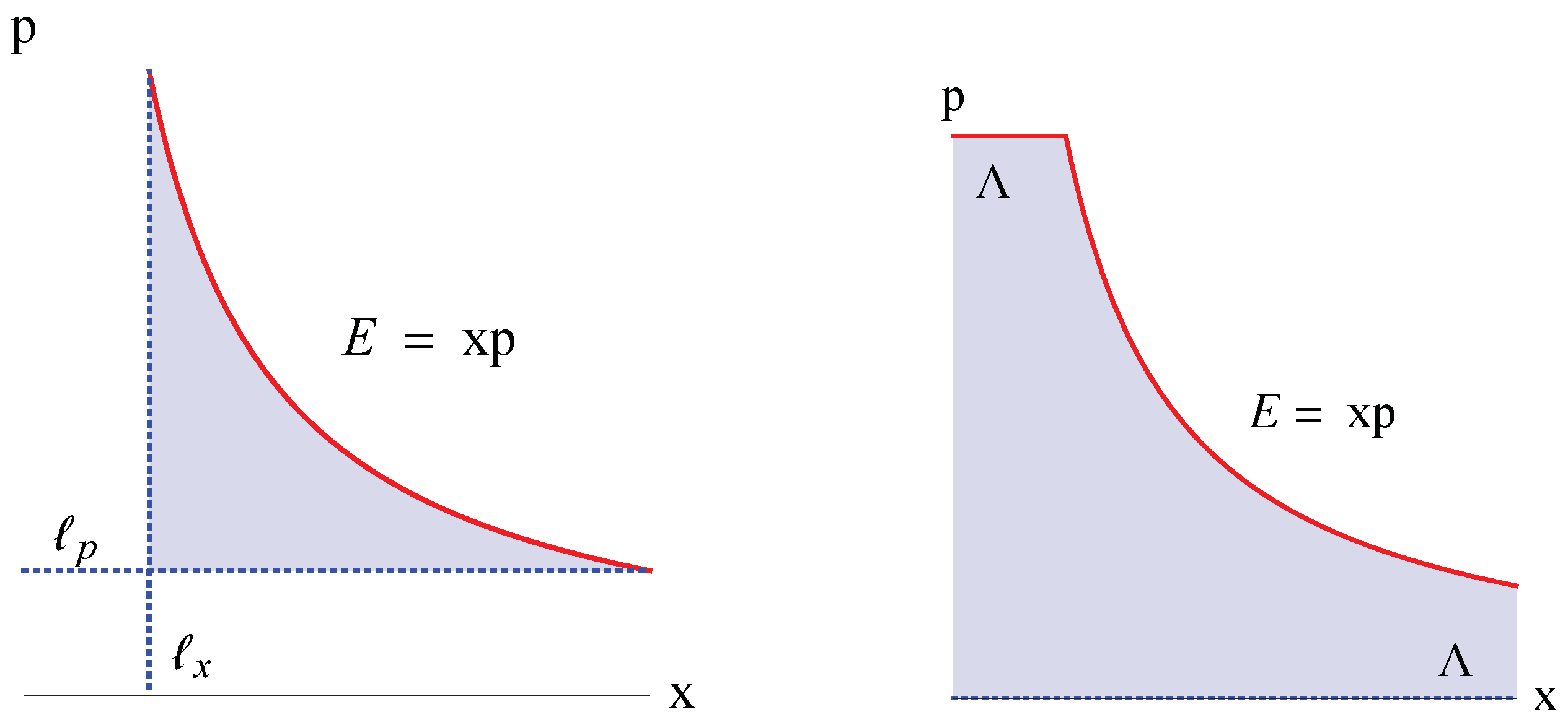
In this section, we review the main results concerning the classical and semiclassical $xp$ model [18,19,20]. A classical trajectory of the Hamiltonian $H_{}=xp$, with energy E, is given by

$$x\left(t\right)=x_0{e}^t,p\left(t\right)=p_0{e}^{-t},E=x_0{p}_0,$$

(1)

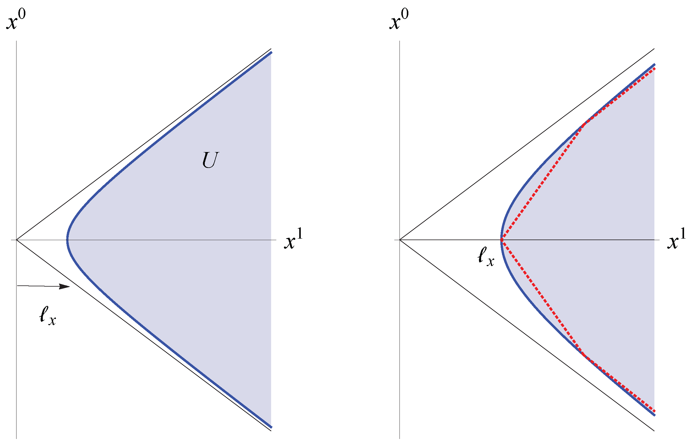
that traces the parabola $E=xp$ in phase space plotted in Figure 1. E has the dimension of an action, so one should multiply $xp$ by a frequency to get an energy, but for the time being we keep the notation $H=xp$. Under a time reversal transformation, $x\to x,p\to -p$ one finds $xp\to -xp$, so that this symmetry is broken. This is why reversing the time variable t in (1) does not yield a trajectory generated by $xp$. As $t\to \infty$, the trajectory becomes unbounded that is $|x|\to \infty$, so one expects the semiclassical and quantum spectrum of the $xp$ model to form a continuum. To get a discrete spectrum Berry and Keating introduced the constraints $|x|\ge {\ell }_x$ and $|p|\ge {\ell }_p$, so that the particle starts at $t=0$ at $(x,p)=({\ell }_x,E/{\ell }_x)$ and ends at $(x,p)=(E/{\ell }_p,{\ell }_p)$ after a time lapse $T=log(E/{\ell }_x{\ell }_p)$ (we assume for simplicity that $x,p>0$). The trajectories are now bounded, but not periodic. A semiclassical estimate of the number of energy levels, $n_{\mathrm{BK}}\left(E\right)$, between 0 and $E>0$ is given by the formula

$$n_{\mathrm{BK}}\left(E\right)=\frac{A_{\mathrm{BK}}}{2\pi \hslash }=\frac{E}{2\pi \hslash }\left(log\frac{E}{{\ell }_x{\ell }_p}-1\right)+\frac{7}{8},$$

(2)

where $A_{\mathrm{BK}}$ is the phase space area below the parabola $E=xp$ and the lines $x={\ell }_x$ and $p={\ell }_p$, measured in units of the Planck’s constant $2\pi \hslash$ (see Figure 1). The term $7/8$ arises from the Maslow phase [18]. In the course of the paper, we shall encounter this equation several times with the constant term depending on the particular model.

Berry and Keating compared this result with the average number of Riemann zeros, whose imaginary part is less than t with $t\gg 1$,

$$\langle n\left(t\right)\rangle \simeq \frac{t}{2\pi }\left(log\frac{t}{2\pi }-1\right)+\frac{7}{8}+O(1/t),$$

(3)

finding an agreement with the identifications

$$t=\frac{E}{\hslash },{\ell }_x{\ell }_p=2\pi \hslash .$$

(4)

Thus, the semiclassical energies E, expressed in units of ℏ, are identified with the Riemann zeros, while ${\ell }_x{\ell }_p$ is identified with the Planck’s constant. This result is remarkable given the simplicity of the assumptions. However, one must observe that the derivation of Equation (2) is heuristic, so one goal is to find a consistent quantum version of it.

Connes proposed another regularization of the $xp$ model based on the restrictions $|x|\le \Lambda$ and $|p|\le \Lambda$, where $\Lambda$ is a common cutoff, which is taken to infinity at the end of the calculation [20]. The semiclassical number of states is computed as before yielding (see Figure 1, we set $\hslash =1$)

$$n_{\mathrm{C}}\left(E\right)=\frac{A_{\mathrm{C}}}{2\pi }=\frac{E}{2\pi }log\frac{{\Lambda }^2}{2\pi }-\frac{E}{2\pi }\left(log\frac{E}{2\pi }-1\right).$$

(5)

The first term on the RHS of this formula diverges in the limit $\Lambda \to \infty$, which corresponds to a continuum of states. The second term is minus the average number of Riemann zeros, which according to Connes, become missing spectral lines in the continuum [17,20]. This is called the absorption spectral interpretation of the Riemann zeros, as opposed to the standard emission spectral interpretation where the zeros form a discrete spectrum. Connes, relates the minus sign in Equation (5) to a minus sign discrepancy between the fluctuation term of the number of zeros and the associated formula in the theory of Quantum Chaos. We shall show below that the negative term in Equation (5) must be seen as a finite size correction of discrete energy levels and not as an indication of missing spectral lines.

Let us give for completeness the formula for the exact number of zeros up to t [2,3]

$$\begin{array}{ccc}\hfill n_{\mathrm{R}}\left(t\right)& =& \langle n\left(t\right)\rangle +n_{\mathrm{fl}}\left(t\right),\hfill \\ \hfill \langle n\left(t\right)\rangle & =& \frac{\theta \left(t\right)}{\pi }+1,n_{\mathrm{fl}}\left(t\right)=\frac{1}{\pi }\mathrm{Im}log\zeta \left(\frac{1}{2}+it\right),\hfill \end{array}$$

(6)

where $\langle n\left(t\right)\rangle$ is the Riemann–von Mangoldt formula that gives the average behavior in terms of the function $\theta \left(t\right)$

$$\begin{array}{ccc}\hfill \theta \left(t\right)& =& \mathrm{Im}log\Gamma \left(\frac{1}{4}+\frac{it}{2}\right)-\frac{t}{2}log\pi \stackrel{t\to \infty }{⟶}\frac{t}{2}log\frac{t}{2\pi }-\frac{t}{2}-\frac{\pi }{8}+O(1/t),\hfill \end{array}$$

(7)

that can also be written as

$$e^{2i\theta \left(t\right)}={\pi }^{-it}\frac{\Gamma \left(\frac{1}{4}+\frac{it}{2}\right)}{\Gamma \left(\frac{1}{4}-\frac{it}{2}\right)}.$$

(8)

$\theta \left(t\right)$ is the phase of the Riemann zeta function on the critical line, that can be expressed as

$$\zeta \left(\frac{1}{2}+it\right)=e^{-i\theta \left(t\right)}Z\left(t\right),$$

(9)

where $Z\left(t\right)$ is the Riemann-Siegel zeta function, or Hardy function, that on the critical line satisfies

$$Z\left(t\right)=Z(-t)=Z^{*}\left(t\right),t\in \mathrm{I}\mathrm{R}.$$

(10)

Summary:

√ The semiclassical spectrum of the $xp$ Hamiltonian reproduces the average Riemann zeros. ✕ There are two schemes leading to opposite physical realizations: emission vs absorption. ? Quantum version of the semiclassical $xp$ models.

3. The Quantum $\mathit{XP}$ Model

To quantize the $xp$ Hamiltonian, Berry and Keating used the normal ordered operator [18]

$$\widehat{H}=\frac{1}{2}(x\widehat{p}+\widehat{p}x)=-i\hslash \left(x\frac{d}{dx}+\frac{1}{2}\right),x\in \mathrm{I}\mathrm{R},$$

(11)

where x belongs to the real line and $\widehat{p}=-i\hslash d/dx$ is the momentum operator. We shall show below that despite of being a natural quantization of the classical $xp$ Hamiltonian, it does not reproduce the semiclassical spectrum obtained in the previous section. It is, however, of great interest to study it in detail since it is the basis of the rest of the work.

It is convenient to restrict x to the positive half-line, then (11) is equivalent to the expression

$$\widehat{H}=\sqrt{x}\widehat{p}\sqrt{x},x\ge 0.$$

(12)

$\widehat{H}$ is an essentially self-adjoint operator acting on the Hilbert space $L^2(0,\infty )$ of square integrable functions in the half-line ${\mathrm{I}\mathrm{R}}_{+}=(0,\infty )$ [23,24,30]. The eigenfunctions, with eigenvalue E, are given by

$${\psi }_E\left(x\right)=\frac{1}{\sqrt{2\pi \hslash }}{x}^{-\frac{1}{2}+\frac{iE}{\hslash }},x>0,E\in \mathrm{I}\mathrm{R},$$

(13)

and the spectrum is the real line $\mathrm{I}\mathrm{R}$. The normalization of (13) is given by the Dirac’s delta function

$$\langle {\psi }_E|{\psi }_{E^{\prime }}\rangle ={\int }_0^{\infty }dx{\psi }_E^{*}\left(x\right){\psi }_{E^{\prime }}\left(x\right)=\delta (E-E^{\prime }).$$

(14)

The eigenfunctions (13) form an orthonormal basis of $L^2(0,\infty )$, that is related to the Mellin transform in the same manner that the eigenfunctions of the momentum operator $\widehat{p}$, on the real line, are related to the Fourier transform [24]. If one takes x in the whole real line, then the spectrum of the Hamiltonian (11) is doubly degenerate. This degeneracy can be understood from the invariance of $xp$ under the parity transformation $x\to -x,p\to -p$, which allows one to split the eigenfunctions with energy E into even and odd sectors

$${\psi }_E^{\left(e\right)}\left(x\right)=\frac{1}{\sqrt{2\pi \hslash }}{|x|}^{-\frac{1}{2}+\frac{iE}{\hslash }},{\psi }_E^{\left(o\right)}\left(x\right)=\frac{\mathrm{sign}x}{\sqrt{2\pi \hslash }}{|x|}^{-\frac{1}{2}+\frac{iE}{\hslash }},x\in \mathrm{I}\mathrm{R},E\in \mathrm{I}\mathrm{R}.$$

(15)

Berry and Keating computed the Fourier transform of the even wave function ${\psi }_E^{\left(e\right)}\left(x\right)$ [18]

$$\begin{array}{ccc}\hfill {\widehat{\psi }}_E^{\left(e\right)}\left(p\right)& =& \frac{1}{\sqrt{2\pi \hslash }}{\int }_{-\infty }^{\infty }dx{\psi }_E^{\left(e\right)}\left(x\right)e^{-ipx/\hslash }\hfill \\ & =& \frac{1}{\sqrt{2\pi \hslash }}{|p|}^{-\frac{1}{2}-\frac{iE}{\hslash }}{(2\hslash )}^{iE/\hslash }\frac{\Gamma \left(\frac{1}{4}+\frac{iE}{2\hslash }\right)}{\Gamma \left(\frac{1}{4}-\frac{iE}{2\hslash }\right)},\hfill \end{array}$$

(16)

which means that the position and momentum eigenfunctions are each other’s time reversed, giving a physical interpretation of the phase $\theta \left(t\right)$, see Equation (8). Choosing odd eigenfunctions leads to an equation similar to Equation (16) in terms of the gamma functions $\Gamma (\frac{3}{4}\pm \frac{iE}{2})$ that appear in the functional relation of the odd Dirichlet L-functions. Equation (16) is a consequence of the exchange $x\leftrightarrow p$ symmetry of the $xp$ Hamiltonian, which is an important ingredient of the $xp$ model.

Comments:

• Removing Connes’s cutoff, i.e., $\Lambda \to \infty$, gives the quantum Hamiltonians (11) or (12), whose spectrum is a continuum. This shows that the negative term in Equation (5) does not correspond to missing spectral lines. In the next section we give a physical interpretation of this term in another context.
• $xp$ is invariant under the scale transformation (dilations) $x\to Kx,p\to K^{-1}p$, with $K>0$. An example of this transformation is the classical trajectory (1), whose infinitesimal generator is $xp$. Under dilations, ${\ell }_x\to K{\ell }_x,{\ell }_p\to K^{-1}{\ell }_p$, so, the condition ${\ell }_x{\ell }_p=2\pi \hslash$ is preserved. Berry and Keating suggested to use integer dilations $K=n$, corresponding to evolution times $logn$, to write [18]

  $${\psi }_E\left(x\right)\to \sum _{n=1}^{\infty }{\psi }_E\left(nx\right)=\frac{1}{\sqrt{2\pi \hslash }}{x}^{-\frac{1}{2}+\frac{iE}{\hslash }}\sum _{n=1}^{\infty }\frac{1}{n^{\frac{1}{2}-\frac{iE}{\hslash }}}=\frac{1}{\sqrt{2\pi \hslash }}{x}^{-\frac{1}{2}+\frac{iE}{\hslash }}\zeta (1/2-iE/\hslash ).$$

  (17)

  If there exists a physical reason for this quantity to vanish one would obtain the Riemann zeros $E_n$. Equation (17) could be interpreted as the breaking of the continuous scale invariance to discrete scale invariance.

Summary:

✕ The normal order quantization of $xp$ does not exhibit any trace of the Riemann zeros. √ The phase of the zeta function appears in the Fourier transform of the $xp$ eigenfunctions.

4. The Landau Model and $\mathit{XP}$

Let us consider a charged particle moving in a plane under the action of a perpendicular magnetic field and an electrostatic potential $V(x,y)\propto xy$ [29]. The Langrangian describing the dynamics is given, in the Landau gauge, by

$$\mathcal{L}=\frac{\mu }{2}({\dot{x}}^2+{\dot{y}}^2)-\frac{eB}{c}\dot{y}x-e\lambda xy,$$

(18)

where $\mu$ is the mass, e the electric charge, B the magnetic field, c the speed of light and $\lambda$ a coupling constant that parameterizes the electrostatic potential. There are two normal modes with real, ${\omega }_c$, and imaginary, ${\omega }_h$, angular frequencies, describing a cyclotronic and a hyperbolic motion respectively. In the limit where ${\omega }_c>>|{\omega }_h|$, only the Lowest Landau Level (LLL) is relevant and the effective Lagrangian becomes

$${\mathcal{L}}_{\mathrm{eff}}=p\dot{x}-|{\omega }_h|xp,p=\frac{\hslash y}{{\ell }^2},\ell ={\left(\frac{\hslash c}{eB}\right)}^{1/2},$$

(19)

where ℓ is the magnetic length, which is proportional to the radius of the cyclotronic orbits in the LLL. The coordinates x and y, which commute in the 2D model, after the projection to the LLL, become canonical conjugate variables, and the effective Hamiltonian is proportional to the $xp$ Hamiltonian with the proportionality constant given by the angular frequency $|{\omega }_h|$ (this is the missing frequency factor mentioned in Section 2). The quantum Hamiltonian associated with the Lagrangian (18) is

$$\widehat{H}=\frac{1}{2\mu }\left[{\widehat{p}}_x+{\left({\widehat{p}}_y+\frac{\hslash }{{\ell }^2}x\right)}^2\right]+e\lambda xy,$$

(20)

where ${\widehat{p}}_x=-i\hslash {\partial }_x$ and ${\widehat{p}}_y=-i\hslash {\partial }_y$. After a unitary transformation (20) becomes the sum of two commuting Hamiltonians corresponding to the cyclotronic and hyperbolic motions alluded to above

$$\begin{array}{ccc}\hfill H& =& H_c+H_h,\hfill \\ \hfill H_c& =& \frac{{\omega }_c}{2}({\widehat{p}}^2+q^2),H_h=\frac{|{\omega }_h|}{2}(\widehat{P}Q+Q\widehat{P}).\hfill \end{array}$$

(21)

In the limit ${\omega }_c\gg |{\omega }_h|$ one has

$${\omega }_c\simeq \frac{eB}{\mu c},|{\omega }_h|\sim \frac{\lambda c}{B}.$$

(22)

The unitary transformation that brings Equation (20) into Equation (21) corresponds to the classical canonical transformation

$$q=x+p_y,p=p_x,Q=-p_y,P=y+p_x.$$

(23)

When ${\omega }_c\gg |{\omega }_h|$, the low energy states of H are the product of the lowest eigenstate of $H_c$, namely $\psi =e^{-q^2/2{\ell }^2}$, times the eigenstates of $H_h$ that can be chosen as even or odd under the parity transformation $Q\to -Q$

$${\Phi }_E^{+}\left(Q\right)=\frac{1}{{|Q|}^{\frac{1}{2}-iE}},{\Phi }_E^{-}\left(Q\right)=\frac{\mathrm{sign}\left(Q\right)}{{|Q|}^{\frac{1}{2}-iE}}.$$

(24)

The corresponding wave functions are given by (we choose $|{\omega }_h|=1$)

$${\psi }_E^{\pm }(x,y)=C\int dQ{e}^{-iQy/{\ell }^2}{e}^{-{(x-Q)}^2/2{\ell }^2}{\Phi }_E^{\pm }\left(Q\right),$$

(25)

where C is a normalization constant, which yields

$$\begin{array}{ccc}\hfill {\psi }_E^{+}(x,y)& =& C_E^{+}{e}^{-\frac{x^2}{2{\ell }^2}}M\left(\frac{1}{4}+\frac{iE}{2},\frac{1}{2},\frac{{(x-iy)}^2}{2{\ell }^2}\right),\hfill \\ \hfill {\psi }_E^{-}(x,y)& =& C_E^{-}(x-iy)e^{-\frac{x^2}{2{\ell }^2}}M\left(\frac{3}{4}+\frac{iE}{2},\frac{3}{2},\frac{{(x-iy)}^2}{2{\ell }^2}\right),\hfill \end{array}$$

(26)

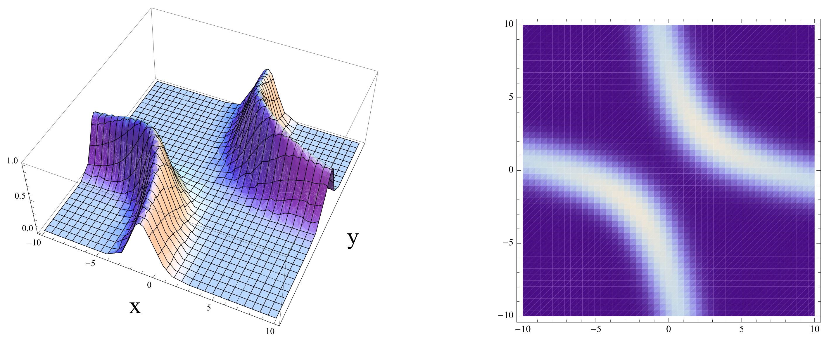
where $M(a,b,z)$ is a confluent hypergeometric function [64]. Figure 2 shows that the maximum of the absolute value of ${\psi }_E^{+}$ is attained on the classical trajectory $E=xy$ (in units of $\hslash =\ell =1$). This 2D representation of the classical trajectories is possible because in the LLL x and y become canonical conjugate variables and consequently the 2D plane coincides with the phase space $(x,p)$.

To count the number of states with an energy below E one places the particle into a box: $|x|<L,|y|<L$ and impose the boundary conditions

$${\psi }_E^{+}(x,L)=e^{ixL/{\ell }^2}{\psi }_E^{+}(L,x),$$

(27)

which identifies the outgoing particle at $x=L$ with the incoming particle at $y=L$ up to a phase. The asymptotic behavior $L\gg \ell$ of (26) is

$$\begin{array}{ccc}\hfill {\psi }_E^{+}(L,x)& \simeq & e^{-ixL/{\ell }^2-x^2/2{\ell }^2}\frac{\Gamma \left(\frac{1}{2}\right)}{\Gamma \left(\frac{1}{4}+\frac{iE}{2}\right)}{\left(\frac{L^2}{2{\ell }^2}\right)}^{-\frac{1}{4}+\frac{iE}{2}},\hfill \\ \hfill {\psi }_E^{+}(x,L)& \simeq & e^{-x^2/2{\ell }^2}\frac{\Gamma \left(\frac{1}{2}\right)}{\Gamma \left(\frac{1}{4}-\frac{iE}{2}\right)}{\left(\frac{L^2}{2{\ell }^2}\right)}^{-\frac{1}{4}-\frac{iE}{2}},\hfill \end{array}$$

(28)

that plugged into the BC (27) yields

$$\frac{\Gamma \left(\frac{1}{4}+\frac{iE}{2}\right)}{\Gamma \left(\frac{1}{4}-\frac{iE}{2}\right)}{\left(\frac{L^2}{2{\ell }^2}\right)}^{-iE}=1,$$

(29)

or using Equation (8)

$$e^{2i\theta \left(E\right)}{\left(\frac{L^2}{2\pi {\ell }^2}\right)}^{-iE}=1.$$

(30)

Hence the number of states $n\left(E\right)$ with energy less that E is given by

$$n\left(E\right)\simeq \frac{E}{2\pi }log\left(\frac{L^2}{2\pi {\ell }^2}\right)+1-\langle n\left(E\right)\rangle ,$$

(31)

whose asymptotic behavior coincides with Connes’s Formula (5) for a cutoff $\Lambda =L/\ell$. In fact, the term $\langle n\left(E\right)\rangle$ is the exact Riemann–von Mangoldt Formula (6).

Summary:

√ The Landau model with a $xy$ potential provides a physical realization of Connes’s $xp$ model. √ The finite size effects in the spectrum are given by the Riemann–von Mangoldt formula. ✕ There are no missing spectral lines in the physical realizations of $xp$ à la Connes.

5. The $\mathit{XP}$ Model Revisited

An intuitive argument of why the quantum Hamiltonian $(x\widehat{p}+\widehat{p}x)/2$ has a continuum spectrum is that the classical trajectories of $xp$ are unbounded. Therefore, to have a discrete spectrum one should modify $xp$ to bound the trajectories. This is achieved by the classical Hamiltonian [32]

$$H_I=x\left(p+\frac{{\ell }_p^2}{p}\right),x\ge {\ell }_x.$$

(32)

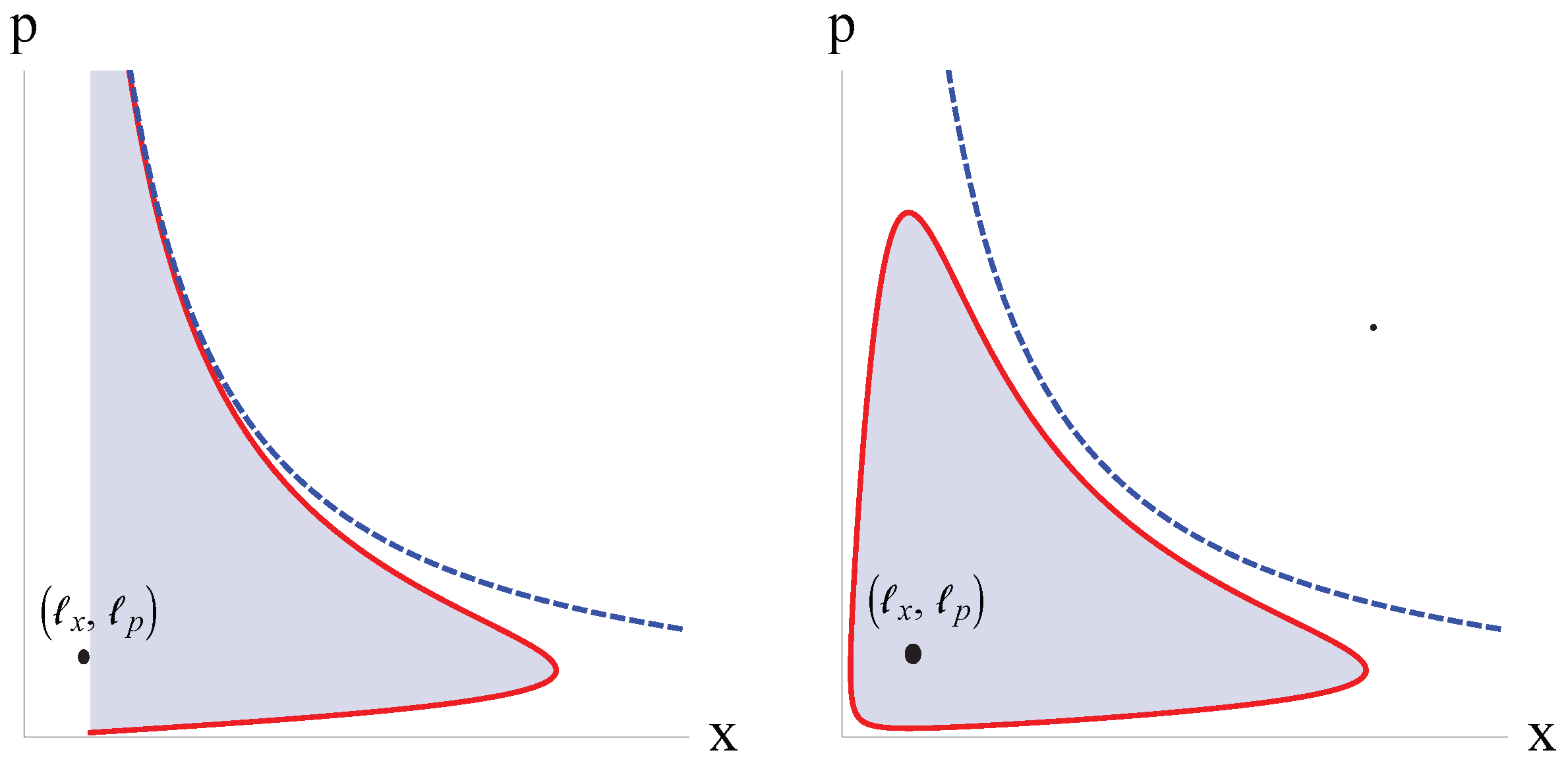
For $|p|>>{\ell }_p$, a classical trajectory with energy E satisfies $E\simeq xp$, but for $|p|\sim {\ell }_p$, the coordinate $|x|$ slows down, reaches a maximum and goes back to the value ${\ell }_x$, where it bounces off starting again at high momentum. In this manner one gets a periodic orbit (see Figure 3)

$$\begin{array}{ccc}\hfill x\left(t\right)& =& \frac{{\ell }_x}{|p_0|}{e}^{2t}\sqrt{(p_0^2+{\ell }_p^2)e^{-2t}-{\ell }_p^2},0\le t\le T_E,\hfill \\ \hfill p\left(t\right)& =& \pm \sqrt{(p_0^2+{\ell }_p^2)e^{-2t}-{\ell }_p^2},\hfill \end{array}$$

(33)

where $T_E$ is the period given by (we take $E>0$)

$$T_E={cosh}^{-1}\frac{E}{2{\ell }_x{\ell }_p}\to log\frac{E}{{\ell }_x{\ell }_p}(E\gg {\ell }_x{\ell }_p).$$

(34)

The asymptotic value of $T_E$ is the time lapse it takes a particle to go from $x={\ell }_x$ to $x=E/{\ell }_p$ in the $xp$ model.

The exchange symmetry $x\leftrightarrow p$ of $xp$ is broken by the Hamiltonian (32). To restore it, Berry and Keating proposed the $x-p$ symmetric Hamiltonian [36]

$$H_{II}=\left(x+\frac{{\ell }_x^2}{x}\right)\left(p+\frac{{\ell }_p^2}{p}\right),x\ge 0.$$

(35)

Here the classical trajectories turn clockwise around the point $({\ell }_x,{\ell }_p)$, and for $x\gg {\ell }_x$ and $p\gg {\ell }_p$, approach the parabola $E=xp$ (see Figure 3). The semiclassical analysis of (32) and (35) reproduce the asymptotic behavior of Equation (2) to leading orders $ElogE$ and E, but differ in the remaining terms.

The two models discussed above have the general form

$$H_{}=U\left(x\right)p+{\ell }_p^2\frac{V\left(x\right)}{p},x\in D,$$

(36)

where $U\left(x\right)$ and $V\left(x\right)$ are positive functions defined in an interval D of the real line. $H_I$ corresponds to $U\left(x\right)=V\left(x\right)=x,D=({\ell }_x,\infty )$, and $H_{II}$ corresponds to $U\left(x\right)=V\left(x\right)=x+{\ell }_x^2/x,D=(0,\infty )$. The classical Hamiltonian (36) can be quantized in terms of the operator

$$\widehat{H}=\sqrt{U}\widehat{p}\sqrt{U}+{\ell }_p^2\sqrt{V}{\widehat{p}}^{-1}\sqrt{V},$$

(37)

where ${\widehat{p}}^{-1}$ is pseudo-differential operator

$$\left({\widehat{p}}^{-1}\psi \right)\left(x\right)=-\frac{i}{\hslash }{\int }_x^{\infty }dy\psi \left(y\right),$$

(38)

which satisfies that $\widehat{p}{\widehat{p}}^{-1}={\widehat{p}}^{-1}\widehat{p}=\mathbf{1}$ acting on functions which vanish sufficiently fast in the limit $x\to \infty$. The action of $\widehat{H}$ is

$$\begin{array}{ccc}\hfill \left(\widehat{H}\psi \right)\left(x\right)& =& -i\hslash \sqrt{U\left(x\right)}\frac{d}{dx}\left\{\sqrt{U\left(x\right)}\psi \left(x\right))\right\}-\frac{i{\ell }_p^2}{\hslash }{\int }_x^{\infty }dy\sqrt{V\left(x\right)V\left(y\right)}\psi \left(y\right).\hfill \end{array}$$

(39)

The normal order prescription that leads from (36) to (39) will be derived in Section 7 in the case where $U\left(x\right)=V\left(x\right)=x$, but holds in general [38]. We want the Hamiltonian (37) to be self-adjoint, that is [65,66]

$$\langle {\psi }_1|\widehat{H}|{\psi }_2\rangle =\langle \widehat{H}{\psi }_1|{\psi }_2\rangle .$$

(40)

When the interval is $D=({\ell }_x,\infty )$, Equation (40) holds for wave functions that vanishes sufficiently fast at infinity and satisfy the non-local boundary condition

$$\hslash e^{i\vartheta }\sqrt{U\left({\ell }_x\right)}\psi \left({\ell }_x\right)={\ell }_p{\int }_{{\ell }_x}^{\infty }dx\sqrt{V\left(x\right)}\psi \left(x\right),$$

(41)

where $\vartheta \in [0,2\pi )$ parameterizes the self-adjoint extensions of $\widehat{H}$. The quantum Hamiltonian associated with (32) is

$${\widehat{H}}_I=\sqrt{x}\widehat{p}\sqrt{x}+{\ell }_p^2\sqrt{x}{\widehat{p}}^{-1}\sqrt{x},x\ge {\ell }_x,$$

(42)

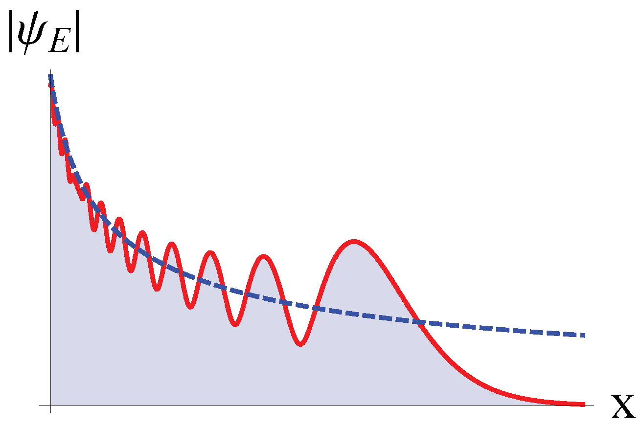
and its eigenfunctions are proportional to (see Figure 4)

$$\begin{array}{ccc}\hfill {\psi }_E\left(x\right)& =& x^{\frac{iE}{2\hslash }}{K}_{\frac{1}{2}-\frac{iE}{2\hslash }}\left(\frac{{\ell }_{p}x}{\hslash }\right)\propto \left\{\begin{array}{cc}{x}^{-\frac{1}{2}+\frac{iE}{\hslash }}\hfill & x\ll \frac{E}{2{\ell }_p},\hfill \\ x^{-\frac{1}{2}+\frac{iE}{2\hslash }}{e}^{-{\ell }_{p}x/\hslash }\hfill & x\gg \frac{E}{2{\ell }_p},\hfill \end{array}\right.\hfill \end{array}$$

(43)

where $K_{\nu }\left(z\right)$ is the modified K-Bessel function [64]. For small values of x, the wave functions (43) behave as those of the $xp$ Hamiltonian, given in Equation (13), while for large values of x they decay exponentially giving a normalizable state. The boundary condition (41) reads in this case

$$\hslash e^{i\vartheta }\sqrt{{\ell }_x}\psi \left({\ell }_x\right)={\ell }_p{\int }_{{\ell }_x}^{\infty }dx\sqrt{x}\psi \left(x\right),$$

(44)

and substituting (43) yields the equation for the eigenenergies $E_n$,

$$e^{i\vartheta }{K}_{\frac{1}{2}-\frac{iE}{2\hslash }}\left(\frac{{\ell }_x{\ell }_p}{\hslash }\right)-K_{\frac{1}{2}+\frac{iE}{2\hslash }}\left(\frac{{\ell }_x{\ell }_p}{\hslash }\right)=0.$$

(45)

For $\vartheta =0$ or $\pi$, the eigenenergies form time reversed pairs $\{E_n,-E_n\}$, and for $\vartheta =0$, there is a zero-energy state $E=0$. Considering that the Riemann zeros form pairs $s_n=1/2\pm i{t}_n$, with $t_n$ real under the RH, and that $s=1/2$ is not a zero of $\zeta \left(s\right)$, we are led to the choice $\vartheta =\pi$. On the other hand, using the asymptotic behavior

$$\begin{array}{ccc}\hfill K_{a+\frac{it}{2}}\left(z\right)& ⟶& \sqrt{\frac{\pi }{t}}{\left(\frac{t}{z}\right)}^a{e}^{-\pi t/4}{e}^{\frac{i\pi }{2}(a-\frac{1}{2})}{\left(\frac{t}{ze}\right)}^{it/2},a>0,t\gg 1,\hfill \end{array}$$

(46)

one derives in the limit $|E|\gg \hslash$,

$$K_{\frac{1}{2}+\frac{iE}{2\hslash }}\left(\frac{{\ell }_x{\ell }_p}{\hslash }\right)+K_{\frac{1}{2}-\frac{iE}{2\hslash }}\left(\frac{{\ell }_x{\ell }_p}{\hslash }\right)=0⟶cos\left(\frac{E}{2\hslash }log\frac{E}{{\ell }_x{\ell }_{p}e}\right)=0,$$

(47)

hence the number of eigenenergies in the interval $(0,E)$ is given asymptotically by

$$n\left(E\right)\simeq \frac{E}{2\pi \hslash }\left(log\frac{E}{{\ell }_x{\ell }_p}-1\right)-\frac{1}{2}+O\left(E^{-1}\right).$$

(48)

This equation agrees with the leading terms of the semiclassical spectrum (2) and the average Riemann zeros (3) under the identifications (4). Concerning the classical Hamiltonian (35), Berry and Keating obtained, by a semiclassical analysis, the asymptotic behavior of the counting function $n\left(E\right)$

$$n_{}\left(t\right)\simeq \frac{t}{2\pi }\left(log\frac{t}{2\pi }-1\right)-\frac{8\pi }{t}log\frac{t}{2\pi }+\dots ,t\gg 1,$$

(49)

where $t=E/\hslash$ and ${\ell }_x{\ell }_p=2\pi \hslash$. Again, the first two leading terms agree with Riemann’s Formula (3), while the next leading corrections are different from (48). In both cases, the constant $7/8$ in Riemann’s Formula (3) is missing.

Summary:

√ The Berry–Keating $xp$ model can be implemented quantum mechanically. ✕ The classical $xp$ Hamiltonian must be modified with ad-hoc terms to have bounded trajectories. ✕ In the quantum theory the latter terms become non-local operators. ✕ The modified $xp$ quantum Hamiltonian related to the average Riemann zeros is not unique. ✕ There is no trace of the exact Riemann zeros in the spectrum of the modified $xp$ models.

6. The Spacetime Geometry of the Modified $\mathit{XP}$ Models

In this section, we show that the modified $xp$ Hamiltonian (36) is a disguised general theory of relativity [35]. Let us first consider the Langrangian of the $xp$ model,

$$L=p\dot{x}-H=p\dot{x}-xp.$$

(50)

In classical mechanics, where $H=p^2/2m+V\left(x\right)$, the Lagrangian can be expressed solely in terms of the position x and velocity $\dot{x}=dx/dt$. This is achieved by writing the momentum in terms of the velocity by means of the Hamilton equation $\dot{x}=\partial H/\partial p=p/m$. However, in the $xp$ model the momentum p is not a function of the velocity because $\dot{x}=\partial H/\partial p=x$. Hence the Lagrangian (50) cannot be expressed uniquely in terms of x and $\dot{x}$. The situation changes radically for the Hamiltonian (36) whose Lagrangian is given by

$$L=p\dot{x}-H=p\dot{x}-U\left(x\right)p-{\ell }_p^2\frac{V\left(x\right)}{p}.$$

(51)

Here the equation of motion

$$\dot{x}=\frac{\partial H}{\partial p}=U\left(x\right)-{\ell }_p^2\frac{V\left(x\right)}{p^2},$$

(52)

allows one to write p in terms of x and $\dot{x}$,

$$p=\eta {\ell }_p\sqrt{\frac{V\left(x\right)}{U\left(x\right)-\dot{x}}},\eta =\mathrm{sign}p,$$

(53)

where $\eta =\pm 1$ is the sign of the momentum that is a conserved quantity. The positivity of $U\left(x\right)$ and $V\left(x\right)$, imply that the velocity $\dot{x}$ must never exceed the value of $U\left(x\right)$. Substituting (53) back into (51), yields the action

$$S_{\eta }=-{\ell }_p\eta \int \sqrt{-d{s}^2},$$

(54)

which, for either sign of $\eta$, is the action of a relativistic particle moving in a 1+1 dimensional spacetime metric

$$d{s}^2=4V\left(x\right)(-U\left(x\right)d{t}^2+dtdx).$$

(55)

The parameter ${\ell }_p$ plays the role of $mc$ where m is the mass of the particle and c is the speed of light. This result implies that the classical trajectories of the Hamiltonian (36) are the geodesics of the metric (55). The unfamiliar form of (36) is due to a special choice of spacetime coordinates where the component $g_{xx}$ of the metric vanishes. A diffeomorphism of x permits to set $V\left(x\right)=U\left(x\right)$. The scalar curvature of the metric (55), in this gauge, is

$$R\left(x\right)=-2\frac{{\partial }_x^{2}V\left(x\right)}{V\left(x\right)},$$

(56)

and vanishes for the models $V\left(x\right)=x$ and $V\left(x\right)=\mathrm{constant}$. For the Hamiltonian (35) one obtains $R\left(x\right)=-4{\ell }_x^2/\left(x(x^2+{\ell }_x^2)\right)$ which vanishes asymptotically.

The flatness of the metric associated with the Hamiltonian (32) implies the existence of coordinates $x^0,x^1$ where (55) takes the Minkowski form

$$d{s}^2={\eta }_{\mu \nu }d{x}^{\mu }d{x}^{\nu },\mathrm{diag}{\eta }_{\mu \nu }=(-1,1).$$

(57)

The change of variables is given by

$$t=\frac{1}{2}log(x^0+x^1),x=\sqrt{-{\left(x^0\right)}^2+{\left(x^1\right)}^2}.$$

(58)

Let $\mathcal{U}$ denote the spacetime domain of the model. In both coordinates it reads

$$\begin{array}{ccc}\hfill \mathcal{U}& =& \left\{(t,x)|t\in (-\infty ,\infty ),x\ge {\ell }_x\right\}=\left\{(x^0,x^1)|x^0\in (-\infty ,\infty ),x^1\ge \sqrt{{\left(x^0\right)}^2+{\ell }_x^2}\right\}.\hfill \end{array}$$

(59)

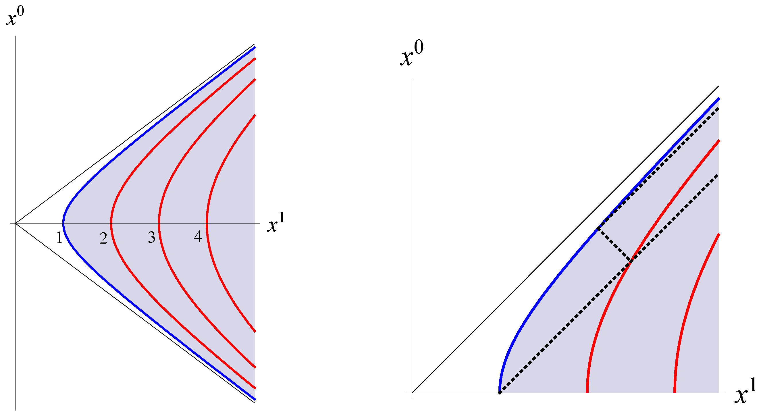
The boundary of $\mathcal{U}$, denoted by $\partial \mathcal{U}$, is the hyperbola $x^1=\sqrt{{\left(x^0\right)}^2+{\ell }_x^2}$, that passes through the point $(x^0,x^1)=(0,{\ell }_x)$, (see Figure 5).

A convenient parametrization of the coordinates $x^{\mu }$ is given by the Rindler variables $\rho$ and $\varphi$ [67]

$$x^0=\rho sinh\varphi ,x^1=\rho cosh\varphi ,$$

(60)

or in light-cone coordinates

$$x^{\pm }=x^0\pm x^1=\pm \rho e^{\pm \varphi },$$

(61)

where the Minkowski metric becomes

$$d{s}^2=-d{x}^{+}d{x}^{-}=d{\rho }^2-{\rho }^{2}d{\varphi }^2.$$

(62)

These coordinates describe the right wedge of Rindler spacetime in 1+1 dimensions

$$\begin{array}{ccc}\hfill {\mathcal{R}}_{+}& =& \left\{(x^0,x^1)|x^0\in (-\infty ,\infty ),x^1\ge |x^0|\right\}=\left\{(\rho ,\varphi )|\varphi \in (-\infty ,\infty ),\rho >0\right\}.\hfill \end{array}$$

(63)

Notice that $\mathcal{U}\subset {\mathcal{R}}_{+}$. The boundary $\partial \mathcal{U}$ corresponds to the hyperbola $\rho ={\ell }_x$ that is the worldline of a particle moving with uniform acceleration equal to $1/{\ell }_x$ (in units $c=1$). The Rindler variables are the ones used to study the Unruh effect [68].

Let us now consider the classical Hamiltonian (35). The underlying metric is given by Equation (55) with $U\left(x\right)=V\left(x\right)=x+{\ell }_x^2/x$. The change of variables

$$t=\frac{1}{2}log(x^0+x^1),x=\sqrt{-{\left(x^0\right)}^2+{\left(x^1\right)}^2-{\ell }_x^2},$$

(64)

brings the metric to the form

$$d{s}^2=\frac{-{\left(x^0\right)}^2+{\left(x^1\right)}^2}{-{\left(x^0\right)}^2+{\left(x^1\right)}^2-{\ell }_x^2}{\eta }_{\mu \nu }d{x}^{\mu }d{x}^{\nu }=\frac{{\rho }^2}{{\rho }^2-{\ell }_x^2}(d{\rho }^2-{\rho }^{2}d{\varphi }^2),\rho \ge {\ell }_x,$$

(65)

which in the limit $\rho \to \infty$ converges to the flat metric (62).

Summary:

√ The classical modified $xp$ models are general relativistic theories in 1+1 dimensions. √ $H=x(p+{\ell }_p^2/p)$ is related to a domain $\mathcal{U}$ of Rindler spacetime. √ $l_p$ is the mass of the particle. √ $1/{\ell }_x$ is the acceleration of a particle whose worldline is the boundary of $\mathcal{U}$. ? Relativistic quantum field theory of the modified $xp$ models.

7. Diracization of $\mathit{H}\mathbf{=}\mathit{X}\mathbf{(}\mathit{P}\mathbf{+}{\mathit{\ell }}_{\mathit{p}}^{\mathbf{2}}\mathbf{/}\mathit{P}\mathbf{)}$

In this section, we show that the Dirac theory provides the relativistic quantum version of the modified $xp$ models [42]. We shall focus on the classical Hamiltonian $H=x(p+{\ell }_p^2/p)$ because the flatness of the associated spacetime makes the computations easier, but the result is general: the quantum Hamiltonian (39) can be derived from the Dirac equation in a curved spacetime with metric (55) [38].

The Dirac action of a fermion with mass m in the spacetime domain (59) is given by (in units $\hslash =c=1$)

$$S=\frac{i}{2}{\int }_{\mathcal{U}}d{x}^{0}d{x}^1\overline{\psi }(\cancel{\partial }+im)\psi ,$$

(66)

where $\psi$ is a two-component spinor, $\overline{\psi }={\psi }^{†}{\gamma }^0$, $\cancel{\partial }={\gamma }^{\mu }{\partial }_{\mu }({\partial }_{\mu }=\partial /\partial x^{\mu })$, and ${\gamma }^{\mu }$ are the 2d Dirac matrices written in terms of the Pauli matrices ${\sigma }^{x,y}$ as

$${\gamma }^0={\sigma }^x,{\gamma }^1=-i{\sigma }^y,\psi =\left(\begin{array}{c}{\psi }_{-}\\ {\psi }_{+}\end{array}\right).$$

(67)

The variational principle applied to (66) provides the Dirac equation

$$(\cancel{\partial }+im)\psi =0,$$

(68)

and the boundary condition

$$\begin{array}{c}\hfill {\dot{x}}^{-}{\psi }_{-}^{†}\delta {\psi }_{-}-{\dot{x}}^{+}{\psi }_{+}^{†}\delta {\psi }_{+}=0,\end{array}$$

(69)

where ${\dot{x}}^{\pm }=d{x}^{\pm }/d\varphi ={\ell }_x{e}^{\pm \varphi }$ is the vector tangent to the boundary $\partial \mathcal{U}$ in the light-cone coordinates $x^{\pm }=x^0\pm x^1$. The Dirac equation reads in components

$$\begin{array}{ccc}\hfill ({\partial }_0-{\partial }_1){\psi }_{+}+im{\psi }_{-}& =& 0,({\partial }_0+{\partial }_1){\psi }_{-}+im{\psi }_{+}=0.\hfill \end{array}$$

(70)

If $m=0$ then ${\psi }_{\pm }$ depends only $x^{\pm }$, and so the fields propagate to the left, ${\psi }_{+}\left(x^{+}\right)$, or to the right, ${\psi }_{-}\left(x^{-}\right)$, at the speed of light. The derivatives in Equation (70) can be written in terms the variables t and x using Equation (58),

$${\partial }_0-{\partial }_1=-\frac{2e^{2t}}{x}{\partial }_x,{\partial }_0+{\partial }_1=e^{-2t}({\partial }_t+x{\partial }_x).$$

(71)

Let us denote by ${\tilde{\psi }}_{\mp }(t,x)$ the fermion fields in the coordinates $t,x$ and by ${\psi }_{\mp }(x^0,x^1)$ the fields in the coordinates $x^0,x^1$. The relation between these fields is given by the transformation law

$${\psi }_{-}={\left(\frac{\partial x}{\partial x^{-}}\right)}^{\frac{1}{2}}{\tilde{\psi }}_{-}={\left(2x\right)}^{-\frac{1}{2}}{e}^t{\tilde{\psi }}_{-},{\psi }_{+}={\left(\frac{\partial x}{\partial x^{+}}\right)}^{\frac{1}{2}}{\tilde{\psi }}_{-}={(x/2)}^{\frac{1}{2}}{e}^{-t}{\tilde{\psi }}_{+}.$$

(72)

Plugging Equations (71) and (72) into (70) gives

$$i{\partial }_t{\tilde{\psi }}_{-}=-i\sqrt{x}{\partial }_x\left(\sqrt{x}{\tilde{\psi }}_{-}\right)+mx{\tilde{\psi }}_{+},{\partial }_x\left(\sqrt{x}{\tilde{\psi }}_{+}\right)=im\sqrt{x}{\tilde{\psi }}_{-}.$$

(73)

The second equation is readily integrated

$${\tilde{\psi }}_{+}(x,t)=-\frac{im}{\sqrt{x}}{\int }_x^{\infty }dy\sqrt{y}{\tilde{\psi }}_{-}(y,t),$$

(74)

and replacing it into the first equation in (73) gives

$$i{\partial }_t{\tilde{\psi }}_{-}(x,t)=-i\sqrt{x}{\partial }_x\left(\sqrt{x}{\tilde{\psi }}_{-}\right)-i{m}^2\sqrt{x}{\int }_x^{\infty }dy\sqrt{y}{\tilde{\psi }}_{-}(y,t).$$

(75)

This is the Schrödinger equation with Hamiltonian (42) and the relation $m={\ell }_p$ found in the previous section. The non-locality of the Hamiltonian (42) is a consequence of the special coordinates $t,x$ where the component ${\tilde{\psi }}_{+}$ becomes non-dynamical and depends non-locally on the component ${\tilde{\psi }}_{-}$ that is identified with the wave function of the modified $xp$ model. Similarly, the boundary condition (44) can be derived from Equation (69) as follows. In Rindler coordinates the latter equation reads

$$\begin{array}{c}\hfill e^{-\varphi }{\psi }_{-}^{†}({\ell }_x,\varphi )\delta {\psi }_{-}({\ell }_x,\varphi )=e^{\varphi }{\psi }_{+}^{†}({\ell }_x,\varphi )\delta {\psi }_{+}({\ell }_x,\varphi ),\forall \varphi ,\end{array}$$

(76)

that is solved by

$$\begin{array}{c}\hfill -i{e}^{i\vartheta }{e}^{-\varphi /2}{\psi }_{-}({\ell }_x,\varphi )=e^{\varphi /2}{\psi }_{+}({\ell }_x,\varphi ),\forall \varphi ,\end{array}$$

(77)

where $\vartheta \in [0,2\pi )$. Using Equation (72) this equation becomes

$$\begin{array}{c}\hfill -i{e}^{i\vartheta }{\tilde{\psi }}_{-}({\ell }_x,t)={\tilde{\psi }}_{+}({\ell }_x,t),\forall t,\end{array}$$

(78)

that together with Equation (74) yields Equation (44). This completes the derivation of the quantum Hamiltonian and boundary condition associated to $H=x(p+{\ell }_p^2/p)$. The eigenfunctions and eigenvalue equation of this model were found in Section 5. However, we shall rederive them in alternative way that will provide new insights in the next section.

Let us start by constructing the plane wave solutions of the Dirac Equation (70),

$$\left(\begin{array}{c}{\psi }_{-}\\ {\psi }_{+}\end{array}\right)\propto \left(\begin{array}{c}{e}^{i\pi /4}{e}^{\beta /2}\\ e^{-i\pi /4}{e}^{-\beta /2}\end{array}\right)e^{i(-p^0{x}^0+p^1{x}^1)},$$

(79)

where $(p^0,p^1)$ is the energy-momentum vector parameterized in terms of the rapidity variable $\beta$

$$\begin{array}{ccc}& & {\left(p^0\right)}^2-{\left(p^1\right)}^2=m^2,\hfill \\ \hfill p^0& =& imsinh\beta ,p^1=imcosh\beta ,\beta \in (-\infty ,\infty ).\hfill \end{array}$$

(80)

In Rindler coordinates these plane wave solutions decay exponentially with the distance as corresponds to a localized wave function

$$e^{i(-p^0{x}^0+p^1{x}^1)}=e^{-m\rho cosh(\beta -\varphi )}\to 0,\mathrm{as}\rho \to \infty .$$

(81)

The general solution of the Dirac equation is given by the linear superposition of plane waves (79). The superposition that reproduces the eigenfunctions of the modified $xp$ model is

$$\begin{array}{ccc}\hfill {\psi }_{\mp }(\rho ,\varphi )& =& e^{\pm i\pi /4}{\int }_{-\infty }^{\infty }d\beta e^{-iE\beta /2}{e}^{\pm \beta /2}{e}^{-m\rho cosh(\beta -\varphi )}\hfill \\ & =& 2e^{\pm i\pi /4}{e}^{(\pm \frac{1}{2}-\frac{iE}{2})\varphi }{K}_{\frac{1}{2}\mp \frac{iE}{2}}\left(m\rho \right),\hfill \end{array}$$

(82)

that replaced in Equation (77) gives

$$e^{i\vartheta }{K}_{\frac{1}{2}-\frac{iE}{2}}\left(m{\ell }_x\right)-K_{\frac{1}{2}+\frac{iE}{2}}\left(m{\ell }_x\right)=0,$$

(83)

which coincides with the eigenvalue Equation (45) with $m={\ell }_p$. Setting $m{\ell }_x=2\pi$ and $\vartheta =\pi$, brings Equation (83) to the form

$${\xi }_H\left(t\right)\equiv K_{\frac{1}{2}+\frac{it}{2}}\left(2\pi \right)+K_{\frac{1}{2}-\frac{it}{2}}\left(2\pi \right)=0.$$

(84)

Summary:

√ The spectrum of a relativistic massive fermion in the domain $\mathcal{U}$ agrees with the average Riemann zeros. ? Does this result provide a hint on a physical realization of the Riemann zeros.

8. $\mathit{\xi }$-Functions: Pólya’s Is Massive and Riemann’s Is Massless

The function ${\xi }_H\left(t\right)$ appearing in Equation (84) reminds the fake$\xi$ function defined by Pólya in 1926 [69,70]

$${\xi }^{*}\left(t\right)=4{\pi }^2\left(K_{\frac{9}{4}+\frac{it}{2}}\left(2\pi \right)+K_{\frac{9}{4}-\frac{it}{2}}\left(2\pi \right)\right).$$

(85)

This function shares several properties with the Riemann $\xi$ function

$$\xi \left(t\right)=\frac{1}{4}s(s-1)\Gamma \left(\frac{s}{2}\right){\pi }^{-s/2}\zeta \left(s\right),s=\frac{1}{2}+it,$$

(86)

namely, ${\xi }^{*}\left(t\right)$ is an entire and even function of t, its zeros lie on the real axis and behave asymptotically like the average Riemann zeros, as shown by the expansion obtained using Equation (46)

$${\xi }^{*}\left(t\right)\stackrel{t\to \infty }{⟶}{2}^{3/4}{\pi }^{-7/4}{t}^{7/4}{e}^{-\pi t/4}cos\left(\frac{t}{2}log\left(\frac{t}{2\pi e}\right)+\frac{7\pi }{8}\right).$$

(87)

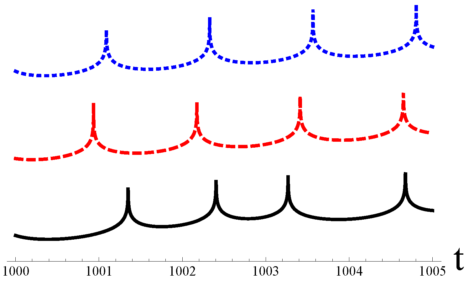
The zeros of $\xi \left(t\right),{\xi }_H\left(t\right)$ and ${\xi }^{*}\left(t\right)$ are plotted in Figure 6. The slight displacement between the two top curves is due to the constant $7\pi /8$ appearing in the argument of the cosine function in Equation (87) as compared to that in Equation (47).

The similarity between ${\xi }_H\left(t\right)$ and ${\xi }^{*}\left(t\right)$, and the relation between ${\xi }^{*}\left(t\right)$ and $\xi \left(t\right)$ provides a hint on the field theory underlying the Riemann zeros. To show this, we shall review how Pólya arrived at ${\xi }^{*}\left(t\right)$. The starting point is the expression of $\xi \left(t\right)$ as a Fourier transform [3]

$$\begin{array}{ccc}\hfill \xi \left(t\right)& =& 4{\int }_1^{\infty }dx\frac{d\left[x^{\frac{3}{2}}{\psi }^{\prime }\left(x\right)\right]}{dx}{x}^{-\frac{1}{4}}cos\left(\frac{tlogx}{2}\right),\hfill \\ \hfill \psi \left(x\right)& =& \sum _{n=1}^{\infty }{e}^{-n^2\pi x},{\psi }^{\prime }\left(x\right)=\frac{d\psi \left(x\right)}{dx}.\hfill \end{array}$$

(88)

In the variable $x=e^{\beta }$ these equations become,

$$\begin{array}{ccc}\hfill \xi \left(t\right)& =& {\int }_0^{\infty }d\beta \Phi \left(\beta \right)cos\frac{t\beta }{2},\hfill \\ \hfill \Phi \left(\beta \right)& =& 2\pi e^{5\beta /4}\sum _{n=1}^{\infty }\left(2\pi e^{\beta }{n}^2-3\right)n^2{e}^{-\pi n^2{e}^{\beta }}.\hfill \end{array}$$

(89)

The function $\Phi \left(\beta \right)$ behaves asymptotically as

$$\Phi \left(\beta \right)\to 4{\pi }^2{e}^{9\beta /4}{e}^{-\pi e^{\beta }},\beta \to \infty ,$$

(90)

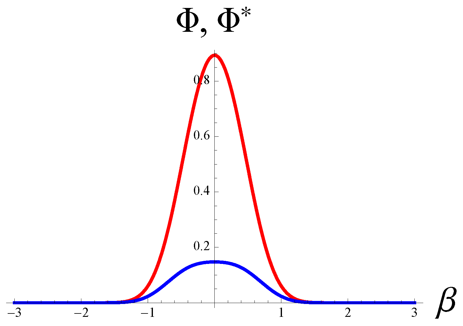
which Pólya replaced by the following expression (see Figure 7).

$${\Phi }^{*}\left(\beta \right)=4{\pi }^2\left(e^{9\beta /4}+e^{-9\beta /4}\right)e^{-\pi (e^{\beta }+e^{-\beta })}.$$

(91)

The function ${\xi }^{*}\left(t\right)$ is defined as the Fourier transform of ${\Phi }^{*}\left(\beta \right)$,

$${\xi }^{*}\left(t\right)={\int }_0^{\infty }d\beta {\Phi }^{*}\left(\beta \right)cos\frac{t\beta }{2},$$

(92)

which finally gives Equation (85). The function (84) can also be written as the Fourier transform

$${\xi }_H\left(t\right)={\int }_0^{\infty }d\beta {\Phi }_H\left(\beta \right)cos\frac{t\beta }{2},$$

(93)

with

$${\Phi }_H\left(\beta \right)=(e^{\beta /2}+e^{-\beta /2})e^{-2\pi cosh\beta }$$

(94)

Observe that the term $e^{-2\pi cosh\beta }$ appears in ${\Phi }_H\left(\beta \right)$ and ${\Phi }^{*}\left(\beta \right)$. The origin of this term in the Dirac theory is the plane wave factor (81) of a fermion with mass m located at the boundary $\rho ={\ell }_x$ with $m{\ell }_x=2\pi$. This observation suggests that the Pólya ${\xi }^{*}$ function arises in the relativistic theory of a massive particle with scaling dimension $9/4$, rather than $1/2$, that corresponds to a fermion (this would explain the different order of the corresponding Bessel functions). The approximation $\Phi \left(\beta \right)\simeq {\Phi }^{*}\left(\beta \right)$, that is $e^{-\pi e^{\beta }}\simeq e^{-2\pi cosh\beta }$, can then be understood as the replacement of a massless particle by a massive one. Indeed, the energy-momentum of a massless right moving particle is given by $p^0=p^1=\Lambda e^{\beta }$, where $\Lambda$ is an energy scale. The corresponding plane wave factor is $e^{-\pi e^{\beta }}$, with $\Lambda =\pi$. For large rapidities, $\beta \gg 1$, a massive particle behaves as a massless one, i.e., $e^{-2\pi cosh\beta }\simeq e^{-\pi e^{\beta }}$. However, for small rapidities this is not the case. These arguments suggest that the field theory underlying the Riemann $\xi$ function, if it exists, must associated with a massless particle.

Summary:

√ The zeros of the Polya ${\xi }^{*}$ function behave as the spectrum of a relativistic massive particle in the domain $\mathcal{U}$. ? Polya’s construction of ${\xi }^{*}$ suggests that the Riemann’s $\xi$ function is related to a massless particle.

9. The Massive Dirac Model in Rindler Coordinates

Let us formulate the Dirac theory in Rindler coordinates. Under a Lorentz transformation with boost parameter $\lambda$, the light-cone coordinates $x^{\pm }$ and the Dirac spinors ${\psi }_{\pm }$ transform as

$$x^{\pm }\to e^{\mp \lambda }{x}^{\pm },{\psi }_{\pm }\to e^{\pm \lambda /2}{\psi }_{\pm },$$

(95)

and the Rindler coordinates (60) as

$$\varphi \to \varphi -\lambda ,\rho \to \rho .$$

(96)

Hence the new spinor fields ${\chi }_{\pm }$ defined as

$${\chi }_{\pm }=e^{\pm \varphi /2}{\psi }_{\pm },$$

(97)

remain invariant under (96). The Rindler wedge ${\mathcal{R}}_{+}$, and its domain $\mathcal{U}$, are also invariant under Lorentz transformations. The Dirac action (66) written in terms of the spinors ${\chi }_{\pm }$ reads

$$\begin{array}{ccc}S& =& \frac{i}{2}{\int }_{-\infty }^{\infty }d\varphi {\int }_{{\ell }_x}^{\infty }d\rho \left[{\chi }_{-}^{†}({\partial }_{\varphi }+\rho {\partial }_{\rho }+\frac{1}{2}){\chi }_{-}+{\chi }_{+}^{†}({\partial }_{\varphi }-\rho {\partial }_{\rho }-\frac{1}{2}){\chi }_{+}+im\rho \left({\chi }_{-}^{†}{\chi }_{+}+{\chi }_{+}^{†}{\chi }_{-}\right)\right],\end{array}$$

(98)

while the Dirac Equation (68) and the boundary condition (77) become

$$({\partial }_{\varphi }\pm \rho {\partial }_{\rho }\pm \frac{1}{2}){\chi }_{\mp }+im\rho {\chi }_{\pm }=0,$$

(99)

and

$$\begin{array}{c}\hfill -i{e}^{i\vartheta }{\chi }_{-}={\chi }_{+}\mathrm{at}\rho ={\ell }_x.\end{array}$$

(100)

The infinitesimal generator of translations of the Rindler time $\varphi$, acting on the spinor wave functions, is the Rindler Hamiltonian $H_R$, which can be read off from (99)

$$i{\partial }_{\varphi }\chi =H_R\chi ,\chi =\left(\begin{array}{c}{\chi }_{-}\\ {\chi }_{+}\end{array}\right),$$

(101)

$$H_R=\left(\begin{array}{cc}-i(\rho {\partial }_{\rho }+\frac{1}{2})& m\rho \\ m\rho & i(\rho {\partial }_{\rho }+\frac{1}{2})\end{array}\right)=\sqrt{\rho }{\widehat{p}}_{\rho }\sqrt{\rho }{\sigma }^z+m\rho {\sigma }^x,$$

(102)

where ${\widehat{p}}_{\rho }=-i\partial /\partial \rho$, is the momentum operator conjugate to the radial coordinate $\rho$. Notice that the operator

$$H_{\rho p_{\rho }}=-i(\rho {\partial }_{\rho }+\frac{1}{2})=\frac{1}{2}(\rho {\widehat{p}}_{\rho }+{\widehat{p}}_{\rho }\rho )=\sqrt{\rho }{\widehat{p}}_{\rho }\sqrt{\rho },$$

(103)

coincides with Equation (11) with the identification $x=\rho$ (in units $\hslash =1$). The eigenfunctions of (103) are

$$H_{\rho p_{\rho }}{\psi }_E=E{\psi }_E,{\psi }_E=\frac{1}{\sqrt{2\pi }}{\rho }^{-1/2+iE},$$

(104)

with real eigenvalue E for $\rho >0$ (recall Equation (13)). Thus, $H_R$ consists of two copies of $xp$, with different signs corresponding to opposite fermion chiralities that are coupled by the mass term $m\rho {\sigma }^x$.

The scalar product of two wave functions, in the domain $\mathcal{U}$, can be defined as

$$\langle {\chi }_1|{\chi }_2\rangle ={\int }_{{\ell }_x}^{\infty }d\rho \left({\chi }_{1,-}^{*}{\chi }_{2,-}+{\chi }_{1,+}^{*}{\chi }_{2,+}\right).$$

(105)

The Hamiltonian $H_R$ is Hermitian with this scalar product acting on wave functions that satisfy Equation (100) and vanish sufficiently fast at infinity, i.e., ${lim}_{\rho \to \infty }{\rho }^{1/2}{\chi }_{\pm }(\rho ,\varphi )=0$. The eigenvalues and eigenvectors of the Hamiltonian (102), are given by the solutions of the Schrödinger equation

$$H_R\chi =E_R\chi ,{\chi }_{\pm }(\rho ,\varphi )=e^{-i{E}_R\varphi \mp i\pi /4}{K}_{\frac{1}{2}\pm i{E}_R}\left(m\rho \right),\rho \ge {\ell }_x,$$

(106)

which coincide with Equation (82) with the identification

$$E_R=\frac{E}{2}.$$

(107)

The factor of $1/2$ comes from the relation $e^{2t}=x^0+x^1=\rho e^{\varphi }$ (see Equation (58)), that implies $e^{-i{E}_R\varphi }\propto e^{-iEt}$. The Rindler eigenenergies are obtained replacing E by $2E_R$ in Equation (83).

Comments:

• The Dirac Hamiltonian associated with the metric (65) is

  $$H=\left(\begin{array}{cc}h& m\rho \Lambda \\ m\rho \Lambda & -h\end{array}\right),h=-i\left(\rho {\partial }_{\rho }+\frac{1}{2}+\frac{1}{2}\rho {\partial }_{\rho }(log\Lambda )\right),\Lambda =\frac{\rho }{\sqrt{{\rho }^2-{\ell }_x^2}}.$$

  (108)

  In the limit $\rho \gg {\ell }_x$ this Hamiltonian converges towards (102).
• Gupta, Harikumar and de Queiroz proposed the Hamiltonian $(x\cancel{p}+\cancel{p}x)/2$ as a Dirac variant of the $xp$ Hamiltonian [37]. The Hamiltonian is defined on a semi-infinite cylinder and effectively becomes one dimensional by considering the winding modes on the compact dimension. The eigenfunctions are given by Whittaker functions and the spectrum satisfies an equation similar to Equation (29) in the Landau theory. In the limit where a regularization parameter goes to zero one obtains a continuum spectrum with a correction term related to the Riemann–von Mangoldt formula.
• Bender, Brody and Müller proposed recently a generalization of the $xp$ operator [43]

  $$H=\frac{\mathbf{1}}{\mathbf{1}-e^{-i\widehat{p}}}(x\widehat{p}+\widehat{p}x)(\mathbf{1}-e^{-i\widehat{p}}),$$

  (109)

  with the property that its eigenvalues $E_n$ give the Riemann zeros as $z_n=\frac{1}{2}(1-i{E}_n)$. This interesting result follows from the fact the eigenfunctions of (109) are given in terms of the Hurwitz zeta function as ${\psi }_z\left(x\right)=\zeta (z,x+1)$ and imposing the boundary condition

  $${\psi }_{z_n}\left(0\right)=0\to \zeta (z_n,1)=\zeta \left(z_n\right)=0.$$

  (110)

  Unfortunately, the operator (109) is not self-adjoint, so that the reality of its eigenvalues is not guaranteed. However, the authors of [43] found that $iH$ has a $PT$ symmetry which, if it is maximally broken, would imply the reality of the eigenvalues. This property though remains to be proved. Further details can be found in references [44,45].

Summary:

√ The massless Dirac Hamiltonian in Rindler spacetime is the direct sum of $xp$ and $-xp$. √ The mass term couples the left and right modes of the fermions.

10. The Massless Dirac Equation with Delta Function Potentials

From analogies between the Polya ${\xi }^{*}$ function, the Riemann $\xi$ function and the ${\xi }_H$ function of the massive Dirac model, we conjectured in Section 8 the existence of a massless field theory underlying $\xi$. At first look this idea does not look correct because the Hamiltonian obtained by setting $m=0$ in Equation (102), is equivalent to two copies of the quantum $xp$ model which has a continuum spectrum. In fact, the mass term in that Hamiltonian is the mechanism responsible for obtaining a discrete spectrum.

To resolve this puzzle, we shall replace the bulk mass term in the Dirac action (98) by a sum of ultra-local interactions placed at fixed values ${\ell }_n$ of the radial coordinate $\rho$ [42]. These interactions can arise from moving mirrors, or beam splitters, that move with a uniform acceleration $1/{\ell }_n$ (see Figure 8). The fermion moves freely, until it hits one of the mirrors and it is reflected or transmitted. The moving mirrors are realized mathematically by delta functions added to the massless Dirac action that couple the left and right components of the fermion on both sides of the mirror. These delta functions provide the matching conditions for the wave functions and can be parameterized by a complex number ${\varrho }_n$ with $n=2,\dots ,\infty$. The scattering of the fermion at each mirror preserves unitarity that is equivalent to the self-adjointness of the Hamiltonian.

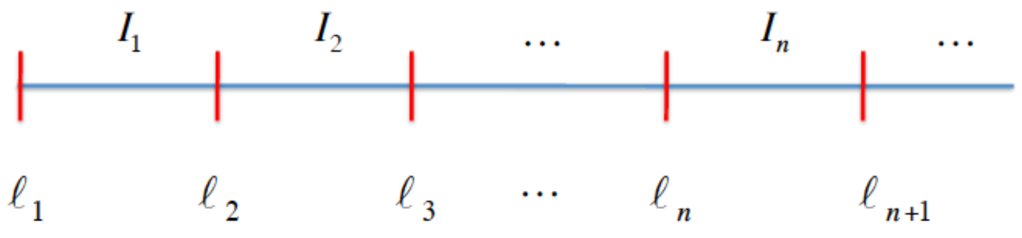
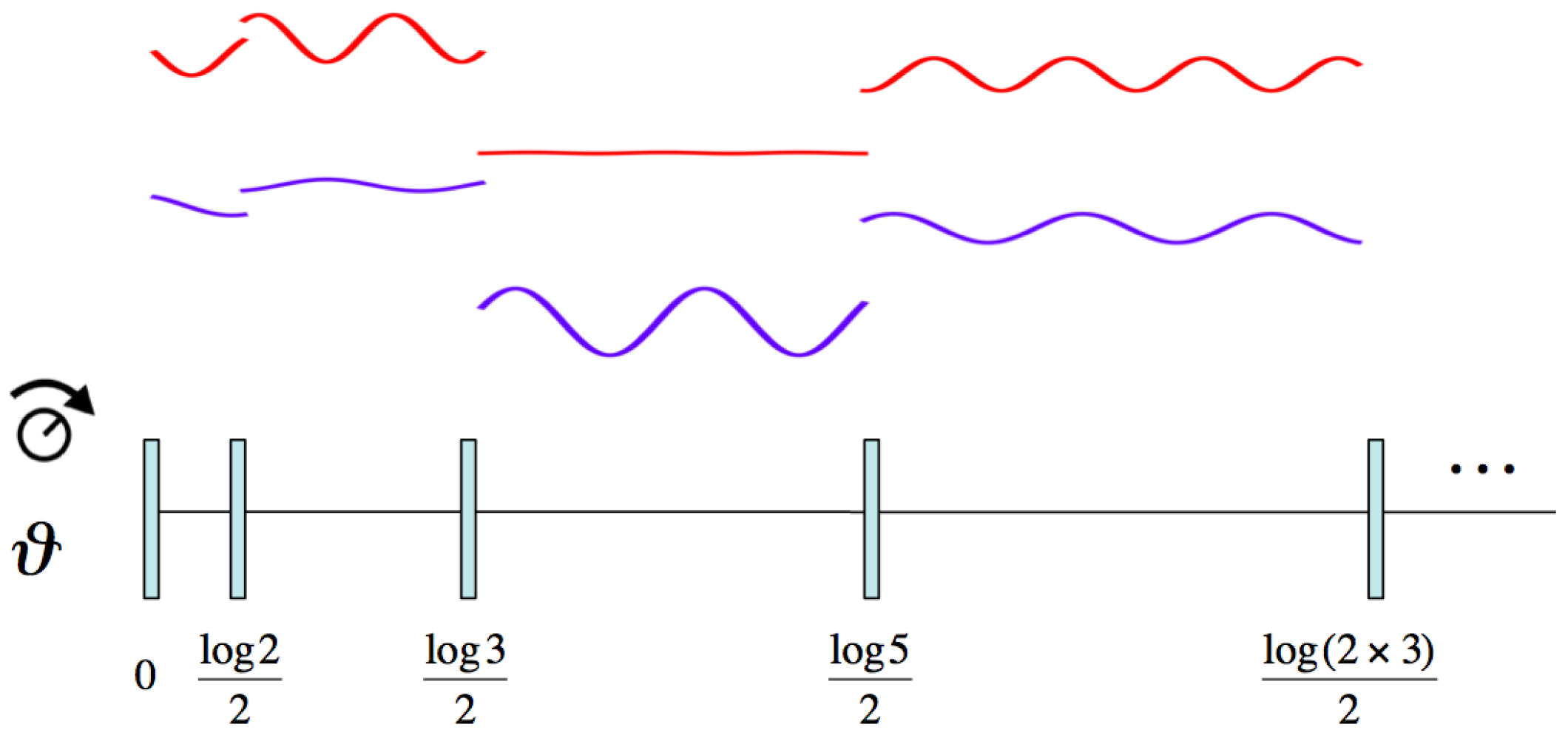
The model is formulated in the spacetime $\mathcal{U}$ defined in Equation (59). We divide $\mathcal{U}$ into an infinite number of domains separated by hyperbolas with constant values of $\rho ={\ell }_n$, as follows. First we define the intervals (see Figure 9)

$$\begin{array}{c}\hfill I_n=\{\rho |{\ell }_n<\rho <{\ell }_{n+1}\},n=1,2,\dots ,\infty ,\end{array}$$

(111)

where using the scale invariance of the model we set ${\ell }_1=1$ (${\ell }_1$ plays the role of ${\ell }_x$ in previous sections).

The partition of $\mathcal{U}$ is given by

$$\begin{array}{ccc}\hfill \mathcal{U}& \to & \tilde{\mathcal{U}}={\cup }_{n=1}^{\infty }{\mathcal{U}}_n,{\mathcal{U}}_n={\mathcal{I}}_n\times \mathrm{I}\mathrm{R},\hfill \end{array}$$

(112)

where the factor $\mathrm{I}\mathrm{R}$ denotes the range of the Rindler time $\varphi$. See Figure 8 for an example with ${\ell }_n=n$. The wave function of the model is the two component Dirac spinor (see Equation (101))

$$\chi \left(\rho \right)=\left(\begin{array}{c}{\chi }_{-}\left(\rho \right)\\ {\chi }_{+}\left(\rho \right)\end{array}\right),\rho \in \mathcal{I}={\cup }_{n=1}^{\infty }{I}_n,$$

(113)

and the scalar product is given by (recall Equation (105))

$$\begin{array}{ccc}\hfill \langle \chi |\chi \rangle & =& \sum _{n=1}^{\infty }{\int }_{{\ell }_n}^{{\ell }_{n+1}}d\rho {\chi }^{†}\left(\rho \right)·\chi \left(\rho \right).\hfill \end{array}$$

(114)

The complex Hilbert space is ${\mathcal{H}}_{}=L^2(\mathcal{I},\mathbb{C})\oplus L^2(\mathcal{I},\mathbb{C})$ and the Hamiltonian is obtained setting $m=0$ in Equation (102)

$$H=\left(\begin{array}{cc}-i(\rho {\partial }_{\rho }+\frac{1}{2})& 0\\ 0& i(\rho {\partial }_{\rho }+\frac{1}{2})\end{array}\right),\rho \notin \mathcal{I}.$$

(115)

H is a self-adjoint operator acting on the subspace ${\mathcal{H}}_{\vartheta }\subset \mathcal{H}$ of wave functions that satisfy the boundary conditions [42] (see [71] for the relation between self-adjointness of operators and boundary conditions)

$$\begin{array}{ccc}\hfill \chi & \in & {\mathcal{H}}_{\vartheta }:\chi \left({\ell }_n^{-}\right)=L\left({\varrho }_n\right)\chi \left({\ell }_n^{+}\right),(n\ge 2),-i{e}^{i\vartheta }{\chi }_{-}\left({\ell }_1^{+}\right)={\chi }_{+}\left({\ell }_1^{+}\right),\hfill \end{array}$$

(116)

where

$$\chi \left({\ell }_n^{\pm }\right)=\underset{\epsilon \to 0^{+}}{lim}\chi ({\ell }_n\pm \epsilon ),$$

(117)

and

$$\begin{array}{ccc}\hfill \vartheta \in [0,2\pi ),L\left(\varrho \right)& =& \frac{1}{1-{|\varrho |}^2}\left(\begin{array}{cc}1+{|\varrho |}^2& 2i\varrho \\ -2i{\varrho }^{*}& 1+{|\varrho |}^2\end{array}\right),\varrho \in \mathbb{C},|\varrho |\ne 1.\hfill \end{array}$$

(118)

This means that H satisfies

$$\begin{array}{c}\hfill \langle {\chi }_1|H{\chi }_2\rangle =\langle H{\chi }_1|{\chi }_2\rangle ,{\chi }_{1,2}\in {\mathcal{H}}_{\vartheta }.\end{array}$$

(119)

This condition guarantees that the norm (114) of the state is conserved by the time evolution generated by the Hamiltonian. The subspace ${\mathcal{H}}_{\vartheta }$ also depends on ${\ell }_n$ and ${\varrho }_n$ but we shall not write this dependence explicitly. Similarly, we shall also denote the Hamiltonian as $H_{\vartheta }$. The matching conditions (116) describe a scattering process where two incoming waves ${\chi }_n^{\mathrm{in}}$ collide at the $n^{\mathrm{th}}$-mirror and become two outgoing waves ${\chi }_n^{\mathrm{out}}$ given by (see Figure 10)

$${\chi }_n^{\mathrm{in}}=\left(\begin{array}{c}{\chi }_{-}\left({\ell }_n^{-}\right)\\ {\chi }_{+}\left({\ell }_n^{+}\right)\end{array}\right),{\chi }_n^{\mathrm{out}}=\left(\begin{array}{c}{\chi }_{-}\left({\ell }_n^{+}\right)\\ {\chi }_{+}\left({\ell }_n^{-}\right)\end{array}\right),n>1.$$

(120)

At the mirror $n=1$, the components ${\chi }_{\pm }\left({\ell }_1^{-}\right)$ of these vectors are null, i.e., there is no propagation at the left of the boundary. The scattering process is described by the matrix $S_n$

$${\chi }_n^{\mathrm{out}}=S_n{\chi }_n^{\mathrm{in}},S_n=\frac{1}{1+|{\varrho }_n{|}^2}\left(\begin{array}{cc}1-|{\varrho }_n{|}^2& -2i{\varrho }_n\\ -2i{\varrho }_n^{*}& 1-|{\varrho }_n{|}^2\end{array}\right),n>1,$$

(121)

that is unitary,

$$S_n{S}_n^{†}=\mathbf{1}.$$

(122)

Notice that the boundary condition at $\rho ={\ell }_1$, is also described by Equation (121) with a parameter ${\varrho }_1$

$${\varrho }_1=-e^{-i\vartheta },$$

(123)

that is a pure phase for the Hamiltonian $H_{\vartheta }$ to be self-adjoint. The matrix $L\left(\varrho \right)$ satisfies

$$L(1/{\varrho }^{*})=-L\left(\varrho \right).$$

(124)

Hence, replacing ${\varrho }_n$ by $1/{\varrho }_n^{*}$ gives a unitary equivalent model because the sign changes at $\rho ={\ell }_n$, given in Equation (124), can be compensated by changing the sign of the wave function in the remaining intervals. Hence, without losing generality, we shall impose the condition $|{\varrho }_n|<1,\forall n>1$.

The eigenfunctions of the Hamiltonian (115) are the customary functions (see Equation (13))

$$H\chi =E\chi ⟶{\chi }_{\mp }\propto {\rho }^{-1/2\pm iE}.$$

(125)

From now one, we shall assume that E is a real number which is guaranteed by the self-adjointness of the Hamiltonian H. In the $n^{\mathrm{th}}$ interval we take

$${\chi }_{\mp ,n}\left(\rho \right)=e^{\pm i\pi /4}\frac{A_{\mp ,n}}{{\rho }^{1/2\mp iE}},{\ell }_n<\rho <{\ell }_{n+1},$$

(126)

where $A_{\mp ,n}$ are constants that in general will depend on E. The phases $e^{\pm i\pi /4}$ have been introduced by analogy with those appearing in Equation (106). The boundary values of $\chi$ at $\rho ={\ell }_n^{\pm }(n\ge 1)$ are (see Equation (117))

$$\begin{array}{c}\hfill {\chi }_{\mp }\left({\ell }_n^{+}\right)={\chi }_{\mp ,n}\left({\ell }_n\right)=e^{\pm \frac{i\pi }{4}}\frac{A_{\mp ,n}}{{\ell }_n^{1/2\mp iE}},{\chi }_{\mp }\left({\ell }_n^{-}\right)={\chi }_{\mp ,n-1}\left({\ell }_n\right)=e^{\pm \frac{i\pi }{4}}\frac{A_{\mp ,n-1}}{{\ell }_n^{1/2\mp iE}}.\end{array}$$

(127)

Let us define the vectors

$$|{\mathbf{A}}_n\rangle =\left(\begin{array}{c}{A}_{-,n}\\ A_{+,n}\end{array}\right),n\ge 1.$$

(128)

The boundary conditions (116) together with Equation (127) imply

$$\begin{array}{ccc}\hfill |{\mathbf{A}}_{n-1}\rangle & =& T_n|{\mathbf{A}}_n\rangle (n\ge 2),|{\mathbf{A}}_1\rangle =|{\mathbf{A}}_1\left(\vartheta \right)\rangle =\left(\begin{array}{c}1\\ e^{i\vartheta }\end{array}\right),\hfill \end{array}$$

(129)

where the transfer matrix $T_n$ is given by

$$\begin{array}{ccc}\hfill T_n& =& \frac{1}{1-|{\varrho }_n{|}^2}\left(\begin{array}{cc}1+|{\varrho }_n{|}^2& 2{\varrho }_n{\ell }_n^{-2iE}\\ 2{\varrho }_n^{*}{\ell }_n^{2iE}& 1+|{\varrho }_n{|}^2\end{array}\right)(n\ge 2).\hfill \end{array}$$

(130)

The norm of the eigenstate can be computed using Equations (114) and (126)

$$\begin{array}{c}\hfill {||\chi ||}^2=\sum _{n=1}^{\infty }log\frac{{\ell }_{n+1}}{{\ell }_n}\langle {\mathbf{A}}_n|{\mathbf{A}}_n\rangle ,\langle {\mathbf{A}}_n|{\mathbf{A}}_n\rangle =|A_{-,n}{|}^2+{|A_{+,n}|}^2.\end{array}$$

(131)

The log term comes from the integral of the norm of the wave function in the $n^{\mathrm{th}}$ interval, ${\int }_{{\ell }_n}^{{\ell }_{n+1}}d\rho /\rho$ (we used that E is real). If ${\varrho }_n=0$ then $T_n=\mathbf{1}$ which implies that $|{\mathit{A}}_{n-1}\rangle =|{\mathit{A}}_n\rangle$. If this happens for all n, then $|{\mathit{A}}_n\rangle =|{\mathit{A}}_1\rangle$, in which case the norm of these states diverges, but they can be normalized using Dirac delta functions, so they correspond to scattering states. In the general case, iterating Equation (129) yields $|{\mathit{A}}_n\rangle$ in terms of $|{\mathit{A}}_1\left(\vartheta \right)\rangle$

$$\begin{array}{ccc}\hfill |{\mathbf{A}}_n\rangle & =& T_n^{-1}{T}_{n-1}^{-1}\dots T_2^{-1}|{\mathbf{A}}_1\left(\vartheta \right)\rangle ,n\ge 2.\hfill \end{array}$$

(132)

For special values of ${\ell }_n$ and ${\varrho }_n$ one can find the exact expression of these amplitudes. An example is ${\ell }_n=e^{n/2},{\varrho }_n=\mathrm{cte}$ [42]. To make contact with the Riemann zeros, we shall consider a limit where the reflection coefficients vanish asymptotically.

Summary:

√ The massless Dirac Hamiltonian with delta function potential is solvable by transfer matrix methods. √ The model is completely characterized by the set of parameters ${\{{\ell }_n,{\varrho }_n\}}_{n=2}^{\infty }$ and $\vartheta$.

11. Heuristic Approach to the Spectrum

Let us replace ${\varrho }_n$ by $\epsilon {\varrho }_n$, and consider the limit $\epsilon \to 0$ of the transfer matrix (130)

$$\begin{array}{ccc}\hfill T_n& \simeq & \mathbf{1}+\epsilon {\tau }_n+O\left({\epsilon }^2\right),{\tau }_n=\left(\begin{array}{cc}0& 2{\varrho }_n{\ell }_n^{-2iE}\\ 2{\varrho }_n^{*}{\ell }_n^{2iE}& 0\end{array}\right)(n\ge 2).\hfill \end{array}$$

(133)

Plugging this equation into Equation (132) yields

$$\begin{array}{c}\hfill |{\mathbf{A}}_n\rangle \simeq \left(\mathbf{1}-\epsilon \sum _{m=2}^n{\tau }_m\right)|{\mathbf{A}}_1\left(\vartheta \right)\rangle +O\left({\epsilon }^2\right),n\ge 2,\end{array}$$

(134)

and in components

$$\begin{array}{ccc}\hfill A_{-,n}& \simeq & 1-2\epsilon e^{i\vartheta }\sum _{m=2}^n{\varrho }_m{\ell }_m^{-2iE}+O\left({\epsilon }^2\right),A_{+,n}\simeq e^{i\vartheta }-2\epsilon \sum _{m=2}^n{\varrho }_m^{*}{\ell }_m^{2iE}+O\left({\epsilon }^2\right).\hfill \end{array}$$

(135)

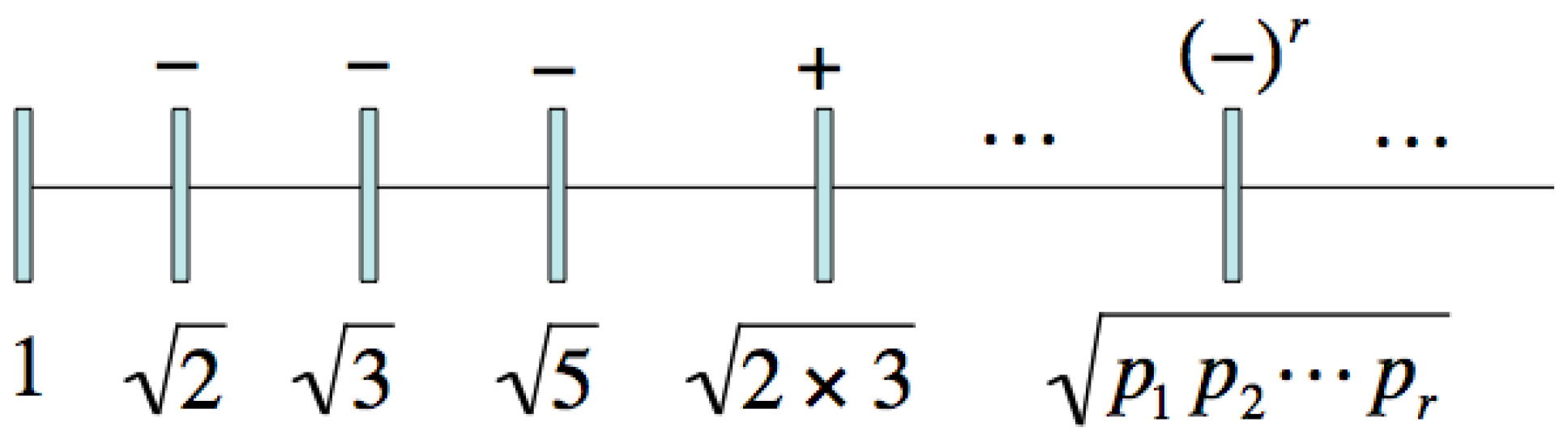
For a normalizable state, the amplitudes $A_{\pm ,n}$ must vanish as $n\to \infty$. In the next section we shall study in detail the normalizability of the state. We shall make the following choice of lengths and reflection coefficients [42]

$${\ell }_n=n^{1/2},{\varrho }_n=\frac{\mu \left(n\right)}{n^{1/2}},n>1,$$

(136)

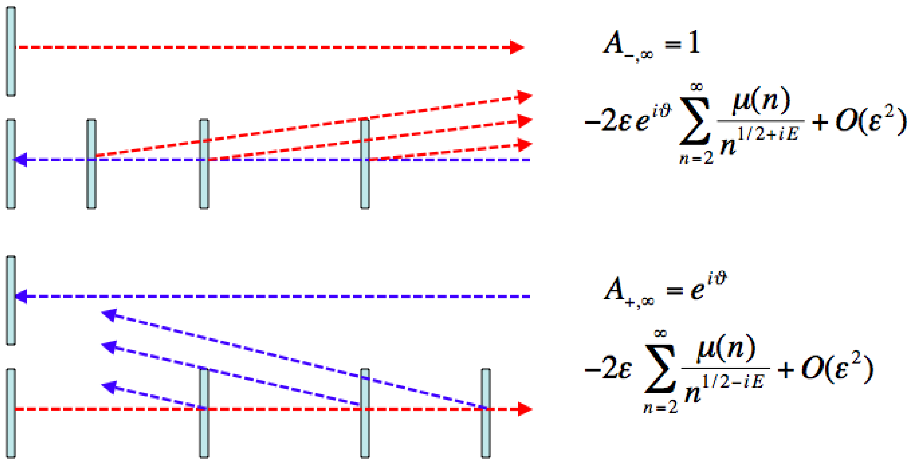
where $\mu \left(n\right)$ is the Moëbius function that is equal to ${(-1)}^r$, with r the number of distinct primes factors of a square free integer n, and $\mu \left(n\right)=0$, if n is divisible by the square of a prime number [4]. See Figure 11 and Figure 12 for a graphical representation of Equations (136) and (135). The Moebius function has been used in the past to provide physical models of prime numbers, most notably in the ideal gas of primons with fermionic statistics [72,73] and a potential whose semiclassical spectrum are the primes [46,74].

Another motivation of the choice (136) is the following [42]. Consider a fermion that leaves the boundary at $\rho ={\ell }_1$, moves rightwards until it hits the mirror at $\rho ={\ell }_n$ where it gets reflected and returns to the boundary. The time lapse for the entire trajectory is given by

$${\tau }_n=2log({\ell }_n/{\ell }_1)$$

(137)

where we used the Rindler metric Equation (62). If the mirror is associated with the prime p, that is ${\ell }_p=\sqrt{p}$, the time will be given by ${\tau }_p=logp$. This result reminds the Berry conjecture that postulates the existence of a classical chaotic Hamiltonian whose primitive periodic orbits are labelled by the primes p, with periods $logp$, and whose quantization will give the Riemann zeros as energy levels [12]. A classical Hamiltonian with this property has not been found, but the array of mirrors presented above, displays some of its properties. In particular, the trajectory between the boundary and the mirror at ${\ell }_p$, with p a prime number, behaves as a primitive orbit with a period $logp$. Moreover, the trajectories and periods of these orbits are independent of the energy of the fermion because it moves at the speed of light.

Let us work out the consequences (136). The condition for a normalizable eigenstate, that is ${lim}_{n\to \infty }{A}_{\pm ,n}=0$, is

$$1\simeq 2\epsilon e^{i\vartheta }\sum _{n=1}^{\infty }\frac{\mu \left(n\right)}{n^{\frac{1}{2}+iE}}=\frac{2\epsilon e^{i\vartheta }}{\zeta (\frac{1}{2}+iE\left(\epsilon \right))},$$

(138)

where we have included the term $n=1$ in the series because it does not modify its value when $\epsilon \to 0$. We have employed the formula ${\sum }_{n=1}^{\infty }\mu \left(n\right)/n^s=1/\zeta \left(s\right)$ for a value of s where the series may not converge. In the next section we shall compute the value of the finite sum that determines the norm of the state. $E_n\left(\epsilon \right)$ denotes a solution such that ${lim}_{\epsilon \to 0}{E}_n\left(\epsilon \right)=E_n$, where $\frac{1}{2}+i{E}_n$ is a zero of the zeta function. All known zeros of $\zeta \left(s\right)$ on the critical line are simple, but we shall also consider the case where $\frac{1}{2}+i{E}_n$ might be a zero of order $r\ge 1$, that is ${\zeta }^{\left(r\right)}\left(s\right)\ne 0$. The Taylor expansion of $\zeta (\frac{1}{2}+iE\left(\epsilon \right))$ around $\frac{1}{2}+i{E}_n$, in Equation (138) yields

$$1\simeq \frac{2\epsilon r!e^{i\vartheta }}{i^r{(E_n\left(\epsilon \right)-E_n)}^r{\zeta }^{\left(r\right)}(\frac{1}{2}+i{E}_n)}.$$

(139)

Hence $E_n\left(\epsilon \right)-E_n$ is of order ${\epsilon }^{1/r}$, as $\epsilon \to 0$ and

$$\frac{{\zeta }^{\left(r\right)}(\frac{1}{2}+i{E}_n)}{{\zeta }^{\left(r\right)}(\frac{1}{2}-i{E}_n)}={(-1)}^r{e}^{2i\vartheta }.$$

(140)

On the other hand, from Equation (9) one finds

$$i^r{\zeta }^{\left(r\right)}(\frac{1}{2}+i{E}_n)=e^{-i\theta \left(E_n\right)}{Z}^{\left(r\right)}\left(E_n\right),$$

(141)

that plugged into (140) yields

$$e^{2i(\vartheta +\theta \left(E_n\right))}=1,\forall r.$$

(142)

We can collect these results in the equation

$$\mathrm{If}\zeta (\frac{1}{2}\pm i{E}_n)=0\mathrm{and}{e}^{2i(\vartheta +\theta \left(E_n\right))}=1⟺H_{\vartheta }{\chi }_{E_n}=E_n{\chi }_{E_n}.$$

(143)

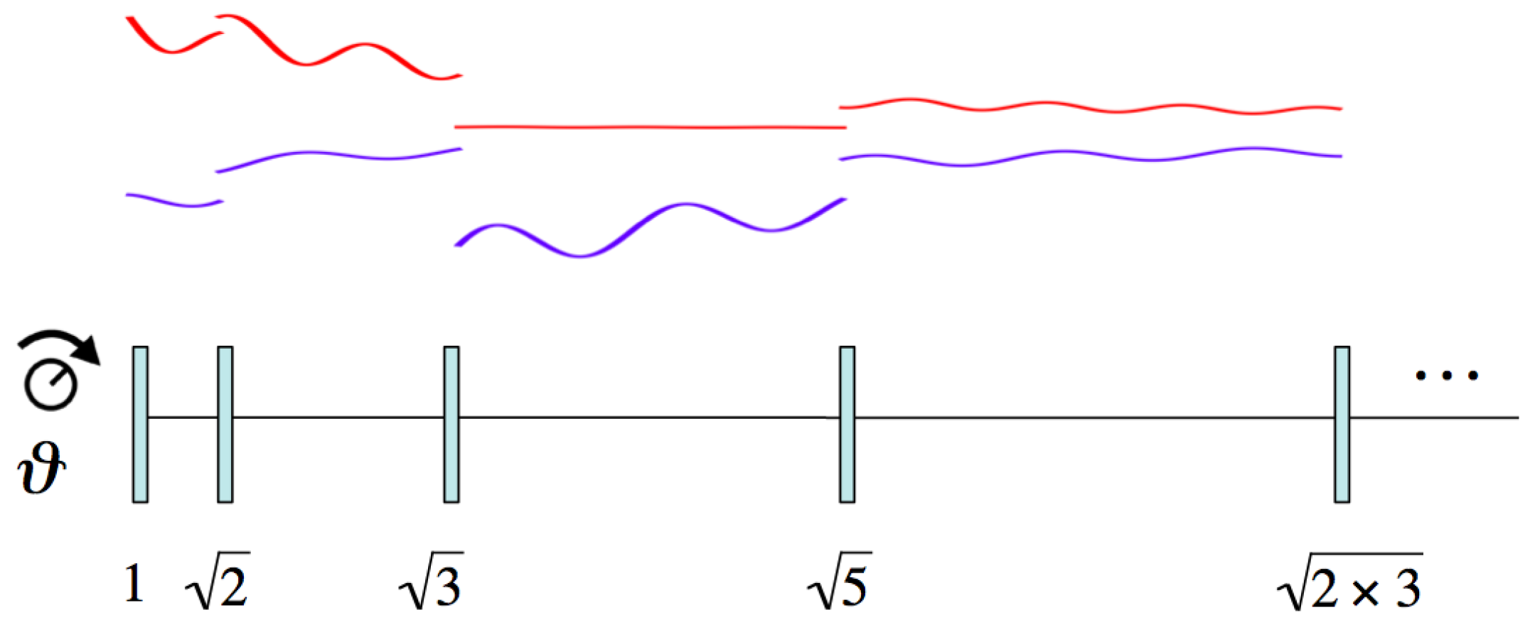
Observe that $\vartheta$ is fixed mod $\pi$. In the next section we shall fix this ambiguity. This equation is heuristic. It has been derived by (i) solving the eigenvalue equation in the limit $\epsilon \to 0$, (ii) imposing the vanishing of the eigenfunction at infinity and (iii) using the Dirichlet series of $1/\zeta \left(s\right)$ in a region where it may not converge. In the next section we shall derive Equation (143) without making the previous assumptions (see Equation (176)). Let us notice that this spectral realization of the zeros requires the fine tuning of the parameter $\vartheta$ in terms of the phase of the zeta function, $\theta \left(E_n\right)$ (see Figure 13). This realization is different from the Pólya-Hilbert conjecture of a single Hamiltonian encompassing all the Riemann zeros at once. This Hamiltonian would exist if $\theta \left(E_n\right)={\theta }_0,\forall n$, but this is certainly not the case.

Summary:

√ A Riemann zero, on the critical line, becomes an eigenvalue of the Hamiltonian $H_{\vartheta }$ by tuning the phase $\vartheta$ according to the phase of the zeta function. ✕ The previous result is obtained in the limit $\epsilon \to 0$ and is heuristic.

12. The Riemann Zeros as Spectrum and the Riemann Hypothesis

In this section, we provide more rigorous arguments that support the heuristic results obtained previously. Let us first review the main properties of the model discussed so far. The Hamiltonian, Equation (115), describes the dynamics of a massless Dirac fermion in the region of Rindler spacetime bounded by the hyperbola $\rho ={\ell }_1$. The reflection of the wave function at this boundary is characterized by a parameter $\vartheta$, which is real for a self-adjoint Hamiltonian. At the positions ${\ell }_{n>1}$ the wave function is discontinuous due to the presence of delta function potentials characterized by the reflection amplitudes ${\varrho }_n$ that provide the matching conditions of the wave function at those sites. An eigenfunction $\chi$, with eigenvalue E, has a simple expression, Equation (126), in terms of the amplitudes $A_{n,\pm }$, which are related by the transfer matrix $T_n$ (130). The norm of $\chi$ is given by the sum of the squared length of the vectors ${\mathbf{A}}_n$, weighted with a factor that depends on the positions ${\ell }_n$, Equation (131). We introduce a scale factor $\epsilon$ in the parameters ${\varrho }_n$, which allows us to study the limit $\epsilon \to 0$, where the mirrors become semitransparent. In this way we found an ansatz for the parameters ${\ell }_n$ and ${\varrho }_n$ that heuristically led to an individual spectral realization of the zeros by fine tuning the parameter $\vartheta$.

12.1. Normalizable Eigenstates

Under the choice ${\ell }_n=n^{1/2}$, Equation (131) becomes

$$\begin{array}{c}\hfill {||\chi ||}^2=\frac{1}{2}\sum _{n=1}^{\infty }log\left(1+\frac{1}{n}\right)\langle {\mathbf{A}}_n|{\mathbf{A}}_n\rangle .\end{array}$$

(144)

This series can be replaced by

$$\begin{array}{c}\hfill {||\chi ||}_c^2\equiv \sum _{n=1}^{\infty }\frac{1}{n}\langle {\mathbf{A}}_n|{\mathbf{A}}_n\rangle ,\end{array}$$

(145)

which is convergent if and only if (144) is convergent. The vectors ${\mathbf{A}}_n$ are obtained by acting on ${\mathbf{A}}_1\left(\vartheta \right)$ with the transfer matrices $T_n$ (see Equation (132)). These matrices have unit determinant and can be written as the exponential of traceless Hermitian matrices, that is,

$$T_n=e^{{\tau }_n},{\tau }_n=\left(\begin{array}{cc}0& r_n{\ell }_n^{-2iE}\\ r_n^{*}{\ell }_n^{2iE}& 0\end{array}\right),\forall E\in \mathrm{I}\mathrm{R},$$

(146)

where taking $|{\varrho }_n|<1$,

$$r_n=\frac{{\varrho }_n}{|{\varrho }_n|}log\frac{1+|{\varrho }_n|}{1-|{\varrho }_n|},{\varrho }_n=\frac{r_n}{|r_n|}tanh\frac{|r_n|}{2}.$$

(147)

To derive Equation (146) we used the relation

$$\exp \left(\begin{array}{cc}0& a\\ b& 0\end{array}\right)=\left(\begin{array}{cc}cosh\left(\sqrt{ab}\right)& \frac{a}{\sqrt{ab}}sinh\left(\sqrt{ab}\right)\\ \frac{b}{\sqrt{ab}}sinh\left(\sqrt{ab}\right)& cosh\left(\sqrt{ab}\right)\end{array}\right),\forall a,b\in \mathbb{C}-\left\{0\right\}.$$

(148)

If $|{\varrho }_n|<<1$ one gets $r_n\simeq 2{\varrho }_n$, hence in that limit both parameters give the same result. Using Equation (146), the recursion relation (132) reads

$$|{\mathbf{A}}_k\rangle =e^{-{\tau }_k}{e}^{-{\tau }_{k-1}}\dots e^{-{\tau }_2}|{\mathbf{A}}_1\rangle ,k\ge 2.$$

(149)

12.2. The Magnus Expansion

It is rather difficult to find an analytic expression of the product of matrices of Equation (149). However, we can estimate it replacing $r_n$ by $\epsilon r_n$, and taking the limit $\epsilon \to 0$. Under this replacement Equation (149) becomes

$$|{\mathbf{A}}_k\rangle =e^{-\epsilon {\tau }_k}{e}^{-\epsilon {\tau }_{k-1}}\dots e^{-\epsilon {\tau }_2}|{\mathbf{A}}_1\rangle (k\ge 2).$$

(150)

The product of exponentials of matrices can be expressed as the exponential of a matrix given by the Magnus expansion [75]

$$e^{-\epsilon {\tau }_k}{e}^{-\epsilon {\tau }_{k-1}}\dots e^{-\epsilon {\tau }_2}=\exp \left(-\epsilon \sum _{n=2}^n{\tau }_n-\frac{{\epsilon }^2}{2}\sum _{n_1>n_2=2}^k[{\tau }_{n_1},{\tau }_{n_2}]+O\left({\epsilon }^3\right)\right)(k\ge 2).$$

(151)

In the limit $\epsilon \to 0$ we truncate this expression to the term of order $\epsilon$,

$$e^{-\epsilon {\tau }_k}{e}^{-\epsilon {\tau }_{k-1}}\dots e^{-\epsilon {\tau }_2}\simeq \exp \left(\begin{array}{cc}0& -\epsilon \sum _{n=2}^k{r}_n{\ell }_n^{-2iE}\\ -\epsilon \sum _{n=2}^k{r}_n^{*}{\ell }_n^{2iE}& 0\end{array}\right)\simeq \exp \left(\begin{array}{cc}0& -\epsilon M_z\left(k\right)\\ -\epsilon M_z^{*}\left(k\right)& 0\end{array}\right),$$

(152)

which using (136)

$$r_n=\frac{\mu \left(n\right)}{n^{1/2}}$$

(153)

gives

$$M_z\left(k\right)=1+\sum _{n=2}^k{r}_n{\ell }_n^{-2iE}=\sum _{n=1}^k\frac{\mu \left(n\right)}{n^z},z=\frac{1}{2}+iE.$$

(154)

We have added the constant 1 to $M_z\left(k\right)$, which does not affect the results in the limit $\epsilon \to 0$. Using Equations (148), (150) and (152) we obtain

$$\begin{array}{ccc}\hfill |{\mathbf{A}}_n\rangle & \simeq & \exp \left(\begin{array}{cc}0& -\epsilon M_z\left(n\right)\\ -\epsilon M_z^{*}\left(n\right)& 0\end{array}\right)\left(\begin{array}{c}1\\ e^{i\vartheta }\end{array}\right)\hfill \\ & =& \left(\begin{array}{cc}cosh(|\epsilon M_z\left(n\right)|)& -\frac{\epsilon M_z\left(n\right)}{|\epsilon M_z\left(n\right)|}sinh(|\epsilon M_z\left(n\right)|)\\ -\frac{\epsilon M_z^{*}\left(n\right)}{|\epsilon M_z\left(n\right)|}sinh(|\epsilon M_z\left(n\right)|& cosh(|\epsilon M_z\left(n\right)|)\end{array}\right)\left(\begin{array}{c}1\\ e^{i\vartheta }\end{array}\right)\hfill \\ & =& \left(\begin{array}{cc}cosh(|\epsilon M_z\left(n\right)|)& -e^{-i{\Phi }_z\left(n\right)}sinh(|\epsilon M_z\left(n\right)|)\\ -e^{i{\Phi }_z\left(n\right)}sinh(|\epsilon M_z\left(n\right)|& cosh(|\epsilon M_z\left(n\right)|)\end{array}\right)\left(\begin{array}{c}1\\ e^{i\vartheta }\end{array}\right)\hfill \\ & \simeq & \left(\begin{array}{c}{e}^{\frac{i}{2}(\vartheta -{\Phi }_z\left(n\right))}\left[e^{-|\epsilon M_z\left(n\right)|}cos(\frac{1}{2}(\vartheta -{\Phi }_z\left(n\right))-i{e}^{|\epsilon M_z\left(n\right)|}sin(\frac{1}{2}(\vartheta -{\Phi }_z\left(n\right))\right]\\ e^{\frac{i}{2}(\vartheta +{\Phi }_z\left(n\right))}\left[e^{-|\epsilon M_z\left(n\right)|}cos(\frac{1}{2}(\vartheta -{\Phi }_z\left(n\right))+i{e}^{|\epsilon M_z\left(n\right)|}sin(\frac{1}{2}(\vartheta -{\Phi }_z\left(n\right))\right]\end{array}\right)(n\ge 2),\hfill \end{array}$$

(155)

where ${\Phi }_z\left(n\right)$ is the phase

$$e^{-i{\Phi }_z\left(n\right)}=\frac{M_z\left(n\right)}{|M_z\left(n\right)|}.$$

(156)

From (155) follows an estimate of the norm (145)

$$\begin{array}{c}\hfill {||\chi ||}_c^2\simeq {\mathcal{N}}_z\left(\epsilon \right)\equiv \sum _{n=1}^{\infty }\frac{1}{n}\left[e^{-2|\epsilon M_z\left(n\right)|}(1+cos(\vartheta -{\Phi }_z\left(n\right))+e^{2|\epsilon M_z\left(n\right)|}(1-cos(\vartheta -{\Phi }_z\left(n\right))\right],\end{array}$$

(157)

whose convergence depends on the asymptotic behavior of $M_z\left(n\right)$ and ${\Phi }_z\left(n\right)$. ${\mathcal{N}}_z\left(\epsilon \right)$ has the lower bound

$${\mathcal{N}}_z\left(\epsilon \right)\ge \sum _{n=1}^{\infty }\frac{2}{n}{e}^{-2|\epsilon M_z\left(n\right)|},$$

(158)

that follows from the inequality

$$a(1+b)+\frac{1}{a}(1-b)\ge 2a,a\in (0,1],b\in [-1,1].$$

(159)

If $|M_z\left(n\right)|$ is bounded then the norm is infinite,

$$\mathrm{if}|M_z\left(n\right)|<C,\forall n⟹{\mathcal{N}}_z\left(\epsilon \right)\ge \sum _{n=1}^{\infty }\frac{2}{n}{e}^{-2|\epsilon |C}=\infty .$$

(160)

This case corresponds in general to eigenstates belonging to the continuum. Eigenstates with finite norm require $|M_z\left(n\right)|$ to be unbounded. Notice that ${\mathcal{N}}_z\left(\epsilon \right)$ is the sum of two series with non-negative terms. The convergence of the first summand in (157) is guaranteed if

$$\sum _{n=1}^{\infty }\frac{1}{n}{e}^{-2|\epsilon M_z\left(n\right)|}<\infty ,$$

(161)

which occurs if $|M_z\left(n\right)|$ diverges sufficiently fast with n. The convergence of the second summand in (157) requires ${\Phi }_z\left(n\right)$ to have a limit when $n\to \infty$, and to choose the parameter $\vartheta$ such that

$$\underset{n\to \infty }{lim}{\Phi }_z\left(n\right)=\vartheta .$$

(162)

Moreover, $1-cos(\vartheta -{\Phi }_z\left(n\right))$ must approach 0 sufficiently fast in order to compensate the factor $\frac{1}{n}{e}^{2\epsilon |M_z\left(n\right)|}$. We now pass to analyze the latter conditions in detail.

12.3. Perron Formula

Let us define the function

$$M_z^{\prime }\left(x\right)\equiv {\sum _{1\le n\le x}}^{\prime }\frac{\mu \left(n\right)}{n^z},z=\frac{1}{2}+iE,E\in \mathrm{I}\mathrm{R},$$

(163)

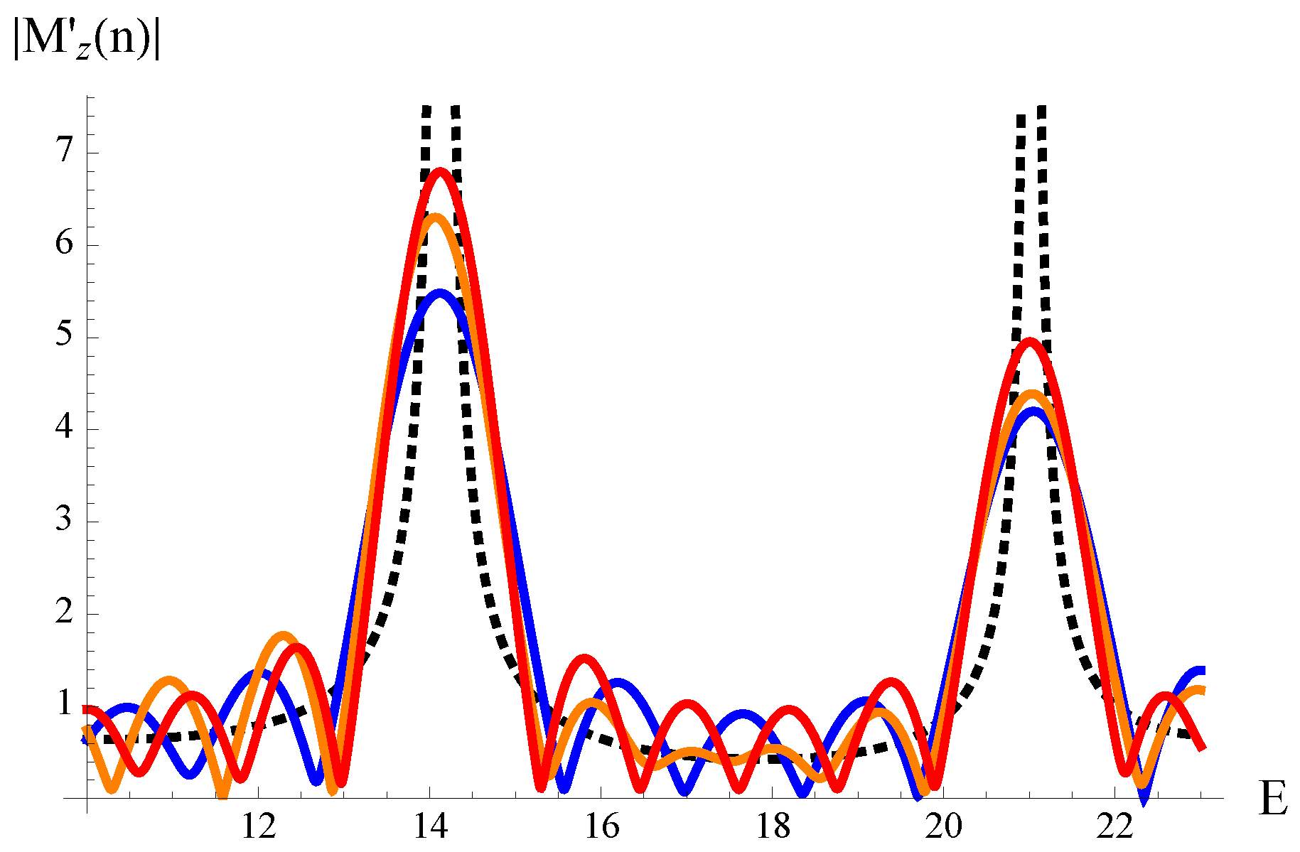
where ${\sum }_{1\le n\le x}^{\prime }$ means that the last term in the sum is multiplied by 1/2 when x is an integer. Figure 14 shows $|M_z^{\prime }\left(n\right)|$ as a function of E for several values of n. Observe that $|M_z^{\prime }\left(n\right)|$ increases with n when E is a zero. We shall derive below this behavior.

To compute $M_z^{\prime }\left(x\right)$ we use Perron’s formula [76]

$$M_z^{\prime }\left(x\right)=\underset{T\to \infty }{lim}{\int }_{c-iT}^{c+iT}\frac{ds}{2\pi i}\frac{1}{\zeta (s+z)}\frac{x^s}{s},c>\frac{1}{2},$$

(164)

where we have used that $\mathrm{Re}z=1/2$. The integral (164) can be done by residue calculus [42]

$$\underset{T\to \infty }{lim}{\int }_{c-iT}^{c+iT}\frac{ds}{2\pi i}F\left(s\right)=\sum _{\mathrm{Re}{s}_j<c}{\mathrm{Res}}_{s_j}F\left(s\right),F\left(s\right)=\frac{1}{\zeta (s+z)}\frac{x^s}{s},$$

(165)

where the sum runs over the poles $s_j$ of $F\left(s\right)$ located to the left of the line of integration $\mathrm{Re}s=c$, which is $\mathrm{Re}{s}_j<c$. The poles of $F\left(s\right)$ come from the zeros of $s\zeta (s+z)$. The pole at $s=0$ can be simple, or multiple, depending on the values of $\zeta \left(z\right)$ and its derivatives. The remaining poles of $F\left(s\right)$ come from the zeros of $\zeta (s+z)$, say $s_j+z={\rho }_j$, and they lie to the left of the integration line, because the trivial and non-trivial zeros of $\zeta$, satisfy $\mathrm{Re}{\rho }_j<1$, which is

$$\mathrm{Re}{s}_j=\mathrm{Re}({\rho }_j-z)=\mathrm{Re}{\rho }_j-\frac{1}{2}<\frac{1}{2}<c.$$

(166)

To compute the residues of Equation (165) we consider the cases: $s=0$, $s_j+z$ a trivial zero of $\zeta$ and $s_j+z$ a non-trivial zero of $\zeta$:

• $s=0$. Let $m\ge 0$ be the lowest integer such that ${\zeta }^{\left(m\right)}\left(z\right)=d^m\zeta \left(z\right)/d{z}^m\ne 0$. Then $F\left(s\right)$ has a pole of order $m+1$ at $s=0$ with residue (The expression for ${\mathrm{Re}}_{s=0}F\left(s\right)$ corresponding to the case $m=1$ contains the term $-\frac{1}{2}{\zeta }^{″}\left(z\right)/{\left({\zeta }^{\prime }\left(z\right)\right)}^2$ which was omitted in the reference [42].)

  $${\mathrm{Res}}_{s=0}F\left(s\right)=\left\{\begin{array}{cc}1/\zeta \left(z\right)\hfill & \mathrm{if}\zeta \left(z\right)\ne 0,\hfill \\ logx/{\zeta }^{\prime }\left(z\right)-\frac{1}{2}{\zeta }^{\prime \prime }\left(z\right)/{\left({\zeta }^{\prime }\left(z\right)\right)}^2\hfill & \mathrm{if}\zeta \left(z\right)=0,{\zeta }^{\prime }\left(z\right)\ne 0.\hfill \\ ⋮\hfill & ⋮\hfill \\ {(logx)}^m/{\zeta }^{\left(m\right)}\left(z\right)+O\left({(logx)}^{m-1}\right)\hfill & \mathrm{if}\zeta \left(z\right)=\dots ={\zeta }^{(m-1)}\left(z\right)=0,{\zeta }^{\left(m\right)}\left(z\right)\ne 0.\hfill \end{array}\right.$$

  (167)
• $s_n=-2n-z(n=1,2,\dots )$, where $F\left(s\right)$ has a simple pole due to the trivial zeros$-2n$ of $\zeta$.

  $${\mathrm{Res}}_{s=-2n-z}F\left(s\right)=\frac{x^{-2n-z}}{-(2n+z){\zeta }^{\prime }(-2n)},n=1,2,\dots ,\infty .$$

  (168)
• $s_j={\rho }_j-z\ne 0$, then $F\left(s\right)$ has a pole due to the non-trivial zero ${\rho }_j$ of $\zeta$

  $${\mathrm{Res}}_{s=s_j}F\left(s\right)=\left\{\begin{array}{cc}\frac{x^{{\rho }_j-z}}{({\rho }_j-z){\zeta }^{\prime }\left({\rho }_j\right)},\hfill & \mathrm{if}\zeta \left({\rho }_j\right)=0,{\zeta }^{\prime }\left({\rho }_j\right)\ne 0\hfill \\ \frac{m{(lnx)}^{m-1}{x}^{{\rho }_j-z}}{({\rho }_j-z){\zeta }^{\left(m\right)}\left({\rho }_j\right)}+O\left({(lnx)}^{m-2}\right),\hfill & \mathrm{if}\zeta \left({\rho }_j\right)=\dots ={\zeta }^{(m-1)}\left({\rho }_j\right)=0,{\zeta }^{\left(m\right)}\left({\rho }_j\right)\ne 0,m\ge 2\hfill \end{array}\right.$$

  (169)

To make further progress we shall assume that all the Riemann zeros are simple, a statement which is not known to hold. The eventual case where there is a zero with double multiplicity will be considered elsewhere. In the former situation we are led to consider only two cases depending on whether z is, or is not, a simple zero of $\zeta$. Collecting terms, we get

$$\begin{array}{ccc}\hfill M_z\left(x\right)& =& \frac{1}{\zeta \left(z\right)}+\sum _{{\rho }_j}\frac{x^{{\rho }_j-z}}{({\rho }_j-z){\zeta }^{\prime }\left({\rho }_j\right)}+\sum _{n=1}^{\infty }\frac{x^{-2n-z}}{-(2n+z){\zeta }^{\prime }(-2n)},\mathrm{if}\zeta \left(z\right)\ne 0,\hfill \end{array}$$

(170)

$$\begin{array}{ccc}{M}_z\left(x\right)& =& \frac{logx}{{\zeta }^{\prime }\left(z\right)}-\frac{{\zeta }^{\prime \prime }\left(z\right)}{2{\left({\zeta }^{\prime }\left(z\right)\right)}^2}+\sum _{{\rho }_j\ne z}\frac{x^{{\rho }_j-z}}{({\rho }_j-z){\zeta }^{\prime }\left({\rho }_j\right)}+\sum _{n=1}^{\infty }\frac{x^{-2n-z}}{-(2n+z){\zeta }^{\prime }(-2n)},\mathrm{if}\zeta \left(z\right)=0,{\zeta }^{\prime }\left(z\right)\ne 0.\end{array}$$

(171)

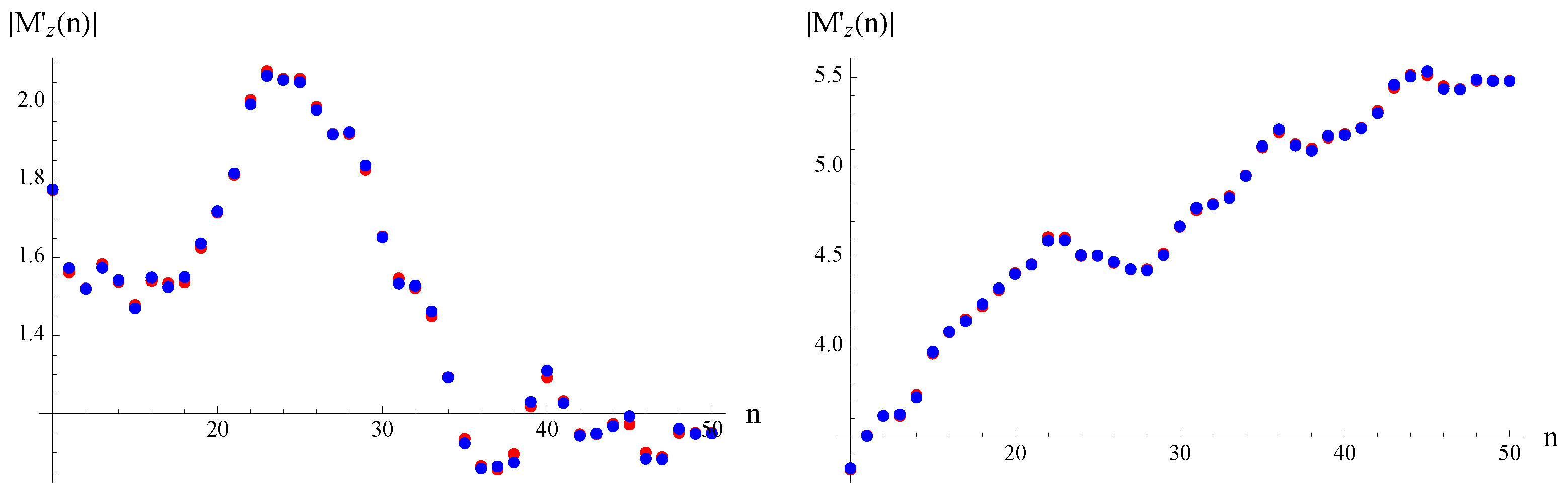
where the sum ${\sum }_{{\rho }_j}$ runs over the non-trivial zeros of $\zeta$. These equations are verified numerically in Figure 15. The last term in these equations, which comes from the trivial zeros, converges quickly and is finite for all x due to the exponential increase of ${\zeta }^{\prime }(-2n)$ [77]

$${\zeta }^{\prime }(-2n)=\frac{{(-1)}^n\zeta (2n+1)\left(2n\right)!}{2^{2n+1}{\pi }^{2n}}\stackrel{n\to \infty }{⟶}{(-1)}^n\sqrt{\pi n}{\left(\frac{n}{e\pi }\right)}^{2n}.$$

(172)

We do not know an estimation of the term depending on the sum over the non-trivial zeros. If the Riemann hypothesis is true the term $x^{{\rho }_j-z}$ will oscillate as a function of x. We expect that for $\zeta \left(z\right)\ne 0$, $|M_z\left(x\right)|$ will not yield a finite norm such that the corresponding eigenstate will not belong to the discrete spectrum. When $\zeta \left(z\right))=0,{\zeta }^{\prime }\left(z\right)\ne 0$, we shall make the approximation

$$\begin{array}{ccc}\hfill M_z\left(x\right)& \to & \frac{logx}{{\zeta }^{\prime }\left(z\right)}x\to \infty ,\hfill \end{array}$$

(173)

where we neglect the finite part $\frac{{\zeta }^{\prime \prime }\left(z\right)}{2{\left({\zeta }^{\prime }\left(z\right)\right)}^2}$; and the possible contribution of the sum over the Riemann zeros. Using that $\zeta (1/2+iE)=e^{-i\theta \left(E\right)}Z\left(E\right)$ we find

$$\begin{array}{ccc}\hfill M_x\left(z\right)& \to & \frac{i{e}^{i\theta \left(E\right)}logx}{Z^{\prime }\left(E\right)}\mathrm{as}x\to \infty ,\hfill \end{array}$$

(174)

hence ${\Phi }_z\left(n\right)$, given in Equation (156), behaves as

$$e^{-i{\Phi }_z\left(n\right)}\to i{e}^{i\theta \left(E\right)}\mathrm{sign}{Z}^{\prime }\left(E\right)\mathrm{as}n\to \infty ,$$

(175)

which has a well-defined asymptotic limit. We shall then choose $\vartheta$ according to Equation (162) namely

$$\vartheta =\underset{n\to \infty }{lim}{\Phi }_z\left(n\right)=-\left(\theta \left(E\right)+\frac{\pi }{2}\mathrm{sign}{Z}^{\prime }\left(E\right)\right),$$

(176)

that provides a necessary condition for the convergence of the norm. It remains to show that Equation (176) is also sufficient but this requires the knowledge of the next to leading correction to (174). Notice that $\vartheta$ depends on $\theta \left(E\right)$ and the sign of $Z^{\prime }\left(E\right)$, a feature that is not left fixed in Equation (142). The norm (157) then becomes

$$\begin{array}{c}\hfill {||\chi ||}_c^2\simeq \sum _{n=1}^{\infty }\frac{2}{n}{e}^{-2\epsilon logn/|Z^{\prime }\left(E\right)|}=2\zeta \left(1+\frac{2\epsilon }{|Z^{\prime }\left(E\right)|}\right)<\infty ,\end{array}$$

(177)

that is finite for all $\epsilon >0$. This result indicates that a zero of the zeta function gives a normalizable state, in agreement with heuristic derivation proposed in the previous section, but there are some differences. First, the eigenvalue E does not need to be expanded in series of $\epsilon$. It is taken to be a zero of $\zeta$ from the beginning. This choice generates the $logx$ term in Equation (171) and is responsible for the finiteness of the norm after the appropriate choice of the phase (176) that also differs from the heuristic value (142). On the other hand, if $\vartheta$ does not satisfy Equation (176), then the norm of the state will diverge badly and so the zero E will be missing in the spectrum. Finally, if E is not a zero, we expect that the state will belong generically to the continuum. Figure 16 shows the expected spectrum of the model, which recalls Connes’s scenario of missing spectral lines, except that in our case, one can pick up a zero at a time by tuning $\vartheta$.

If the RH is false there will be at least four zeros outside the critical line, say ${\rho }_c={\sigma }_c+i{E}_c,{\overline{\rho }}_c={\sigma }_c-i{E}_c,1-{\rho }_c$ and $1-{\overline{\rho }}_c$, with ${\sigma }_c>\frac{1}{2},E_c\in {\mathrm{I}\mathrm{R}}_{+}$. We shall choose the highest value of ${\sigma }_c$. The asymptotic behavior of $M_z\left(x\right)$ will be given by the zeros located to the right of the critical line,

$$\begin{array}{ccc}\hfill M_z\left(x\right)& \to & \frac{x^{{\rho }_c-z}}{({\rho }_c-z){\zeta }^{\prime }\left({\rho }_c\right)}+\frac{x^{{\overline{\rho }}_c-z}}{({\overline{\rho }}_c-z){\zeta }^{\prime }\left({\overline{\rho }}_c\right)}\mathrm{as}x\to \infty .\hfill \end{array}$$

(178)

To simplify the discussion let us choose $E\gg E_c$, which yields the approximation

$$\begin{array}{ccc}\hfill M_z\left(x\right)& \to & \frac{2i{x}^{{\sigma }_c-1/2-iE}}{E|{\zeta }^{\prime }\left({\rho }_c\right)|}cos(E_{c}logx-{\varphi }_c)\mathrm{as}x\to \infty ,\hfill \end{array}$$

(179)

where $e^{i{\varphi }_c}={\zeta }^{\prime }\left({\rho }_c\right)/|{\zeta }^{\prime }\left({\rho }_c\right)|$. The phase ${\Phi }_z\left(n\right)$ is given by Equation (156)

$${\Phi }_z\left(n\right)\to Elogn-\frac{\pi }{2}\mathrm{sign}(cos(E_{c}logn-{\varphi }_c))\mathrm{as}n\to \infty .$$

(180)

Correspondingly, the norm (157) diverges so badly, $\propto {\sum }_n\frac{1}{n}\exp \left(C{n}^{{\sigma }_c-1/2}\right)\dots$, for any value of $\vartheta$ that the state will not be normalizable even using Dirac delta functions. This result occurs for all eigenenergies E. Therefore, the Hamiltonian will not admit a spectral decomposition, but this is impossible because it is a well-defined self-adjoint operator. We conclude that a zero outside the critical line does not exist which provides an argument likely to be persuasive to physicists for the truth of the Riemann hypothesis.

13. The Riemann Interferometer

The model considered in the previous sections looks at first glance quite difficult to simulate. We shall next show that this model is equivalent to another one that can be implemented in the Lab. We shall call this system the Riemann interferometer. The basic idea can be illustrated with the mapping between the quantum $xp$ Hamiltonian and the momentum operator $\widehat{p}$. Let us make the change of coordinates $x=log\rho$ and relate the wave functions in both coordinates, $\varphi \left(x\right)$ and $\psi \left(\rho \right)$, as follows

$$\varphi \left(x\right)={\left(\frac{d\rho }{dx}\right)}^{1/2}\psi \left(\rho \right)=e^{x/2}\psi \left(e^x\right).$$

(181)

An eigenstate of the Hamiltonian $(\rho {\widehat{p}}_{\rho }+{\widehat{p}}_{\rho }\rho )/2$, with eigenvalue E, is mapped by Equation (181) into an eigenstate of the momentum operator ${\widehat{p}}_x=-i{\partial }_x$ with the same eigenvalue,

$$\psi \left(\rho \right)=\frac{1}{{\rho }^{1/2-iE}}⟹\varphi \left(x\right)=e^{iEx}.$$

(182)

This shows that the energy E can be seen as momentum. For a relativistic massless fermion, this is always the case. The measure that defines the scalar product of the corresponding Hilbert spaces are one-to-one related

$${\int }_{\ell }^{\infty }d\rho {\psi }_1^{*}\left(\rho \right){\psi }_2\left(\rho \right)={\int }_{log\ell }^{\infty }dx{\varphi }_1^{*}\left(x\right){\varphi }_2\left(x\right).$$

(183)

The operator $(\rho {\widehat{p}}_{\rho }+{\widehat{p}}_{\rho }\rho )/2$ is self-adjoint in the interval $(0,\infty )$ but not in the interval $(1,\infty )$, just like ${\widehat{p}}_x$ is self-adjoint in the real line $(-\infty ,\infty )$ but not in the half-line $(0,\infty )$ [23,66]. The former case corresponds to the value $\ell =0$ and the latter one to $\ell =1$ in Equation (183). Let us now consider the Dirac Hamiltonian in the Rindler variable $\rho$, given in Equation (115). It becomes in the x variable

$$H=\left(\begin{array}{cc}-i{\partial }_x& 0\\ 0& i{\partial }_x\end{array}\right).$$

(184)

Unlike ${\widehat{p}}_x$, this Hamiltonian is self-adjoint in the interval $x\in (log{\ell }_1,\infty )$. We choose for convenience ${\ell }_1=1$. The moving mirrors located at $\rho ={\ell }_n$ are now placed at the positions $x=d_n$, with $d_n=log{\ell }_n$, so for ${\ell }_n=\sqrt{n}$, we get

$$d_n=\frac{1}{2}logn,$$

(185)

where n are square free integers and the reflection coefficients are given by $r_n=\mu \left(n\right)/\sqrt{n}$. Figure 17 shows the array of mirrors satisfying Equation (185). One can easily generalize this interferometer to provide a spectral realization of the zeros of Dirichlet L-functions, by changing the reflection coefficients $r_n$,

$$L_{\chi }\left(s\right)=\sum _{n=1}^{\infty }\frac{\chi \left(n\right)}{n^s}⟶r_n=\frac{\mu \left(n\right)\chi \left(n\right)}{n^{1/2}},$$

(186)

where $\chi \left(n\right)$ is the Dirichlet character associated with the L-function. It would be interesting to replace the massless fermions by massless bosons, say photons and study what kind of Riemann interferometer arise.

14. Dirac Models for a Class of Modified $\mathit{\zeta }$ and $\mathit{L}$ Functions

Grosswald and Schnitzer proved in 1978 two very surprising theorems that we shall use below to generalize the construction done in the previous sections. Let us first consider a set on integers $q_n$ satisfying the conditions

$$p_n\le q_n\le p_{n+1},n=1,\dots ,\infty ,$$

(187)

where $p_n$ is the $n^{\mathrm{th}}$ prime number. With these numbers define the infinite product

$${\zeta }^{*}\left(s\right)=\prod _{n=1}^{\infty }{(1-q_n^{-s})}^{-1}.$$

(188)

One then has [78]:

Theorem 1.

This function is holomorphic for $\sigma =\mathrm{Re}s>1$ and has the following properties:

$$\begin{array}{cc}\hfill \left(i\right)& {\zeta }^{*}\left(s\right)\ne 0,\mathrm{for}\sigma >1,\hfill \\ \hfill \left(ii\right)& {\zeta }^{*}\left(s\right)\mathrm{has}\mathrm{a}\mathrm{meromorphic}\mathrm{extension}\mathrm{to}\sigma >0,\hfill \\ \hfill \left(iii\right)& \mathrm{in}\sigma >0,{\zeta }^{*}\left(s\right)\mathrm{has}\mathrm{a}\mathrm{simple}\mathrm{pole}\mathrm{at}s=1\mathrm{with}\mathrm{residue}r,1/2\le r\le 1,\hfill \\ \hfill \left(iv\right)& \mathrm{in}\sigma >0,{\zeta }^{*}\left(s\right)\mathrm{has}\mathrm{the}\mathrm{same}\mathrm{zeros}\mathrm{as}\zeta \left(s\right)\mathrm{with}\mathrm{the}\mathrm{same}\mathrm{multiplicity}.\hfill \end{array}$$

This theorem means that the relation between prime numbers and Riemann zeros via the zeta function is less rigid that one may have though. We shall use this freedom to associate a Hamiltonian to every series satisfying (187). Let us first write the inverse of (188) as

$$\frac{1}{{\zeta }^{*}\left(s\right)}=\sum _{n=1}^{\infty }\frac{{\mu }^{*}\left(n\right)}{n^s},{\mu }^{*}\left(n\right)=n_{\mathrm{even}}-n_{\mathrm{odd}},$$

(189)

where $n_{\mathrm{even}}\left(n_{\mathrm{odd}}\right)$ is the number of times n can be written as the product of an even (odd) number of $q_i$ numbers in the series (187). An example of a series satisfying (187) is

$$2,4,6,8,12,\dots q_n=p_n+1,\dots$$

(190)

for which we have

$$\frac{1}{{\zeta }^{*}\left(s\right)}=1-\frac{1}{2^s}-\frac{2}{{(2^6·3)}^s}+\frac{2}{{(2^3·3)}^s}+\frac{1}{{(2^8·3)}^s}-\frac{1}{2^{2s}}-\frac{1}{{(2·3)}^s}+\dots .$$

(191)

Notice that ${\mu }^{*}(2^6·3)=-2$ because $2^6·3=4·6·8=2·8·12$. Obviously ${\mu }^{*}\left(n\right)=\mu \left(n\right)$ if $q_n=p_n,\forall n$. Using Equation (189) we define a massless Dirac model with reflection coefficients (recall Equation (153))

$$r_n=\frac{{\mu }^{*}\left(n\right)}{n^{1/2}},n>1.$$

(192)

Hence, by the arguments given in Section 12 and Theorem 1, we shall find the Riemann zeros in the spectrum of the Hamiltonian $H_{\vartheta }$ by tuning the parameter $\vartheta$ in the limit $\epsilon \to 0$.

The second theorem in reference [78] is an extension of Theorem 1 to Dirichlet L-functions $L\left(s\right)={\prod }_n{(1-\chi \left(n\right)n^{-s})}^{-1}$, where $\chi$ is a character modulo k. The series (187) is replaced by

$$p_n\le q_n\le p_n+K,p_n=q_n\mathrm{mod}k$$

(193)

where $K\ge k$. The modified L-function is defined as

$$L^{*}\left(s\right)=\prod _{n=1}^{\infty }{(1-\chi \left(q_n\right)q_n^{-s})}^{-1},$$

(194)

that can be extended to the region $\sigma >0$, with the same zeros (and multiplicities) as $L\left(s\right)$. In this case, too, we can construct a Dirac model with reflection coefficients (recall Equation (186))

$$r_n=\frac{\chi \left(n\right){\mu }^{*}\left(n\right)}{n^{1/2}},n>1.$$

(195)

whose associated Hamiltonian $H_{\vartheta }$ contains the zeros of $L\left(s\right)$ by varying $\vartheta$. Theorem 2 of [78] was mentioned by LeClair and Mussardo in [63] as a support to their approach to the Generalized Riemann hypothesis based on random walks and the Lemke Oliver-Soundararajan conjecture on the distribution of pairs of residues on consecutive primes [79] (for other statistical properties of the prime numbers see [80,81]). It will be worth to investigate if there is a relation between our approach and the one proposed in [62,63].

15. Conclusions

In this paper, we have reviewed the spectral approach to the RH that started with the Berry–Keating–Connes $xp$ model and continued with several works aimed to provide a physical realization of the Riemann zeros. The main steps in this approach are: (i) spectral realization of Connes’s $xp$ model using the Landau model of an electron in a magnetic field and electrostatic potential, (ii) construction of modified quantum $xp$ models whose spectra reproduce, on average, the behavior of the zeros, (iii) reformulation of the $x(p+1/p)$ model as a relativistic theory of a massive Dirac fermion in a region of Rindler spacetime, (iv) inclusion of prime numbers into the massless Dirac equation by means of delta function potentials acting as moving mirrors that, in the limit where they become semitransparent, leads to a spectral realization of the zeros, (v) a route for proving the Riemann Hypothesis, and (vi) proposal of an interferometer that may provide an experimental observation of the zeros of the Riemann zeta function and other Dirichlet L-functions.

The Pólya-Hilbert (PH) conjecture was proposed as a physical explanation of the RH based on the spectral properties of self-adjoint operators: there exists a single quantum Hamiltonian containing all the Riemann zeros in its spectrum which are therefore real numbers. This statement can be called the global version of the PH conjecture. Instead of this, we have found a local version according to which a Riemann zero $E_n$ becomes an eigenvalue of the Hamiltonian $H_{\vartheta }$ provided the parameter $\vartheta$, which characterizes the self-adjoint extension, is fine-tuned to the combination $\theta \left(E_n\right)+\frac{\pi }{2}\mathrm{sign}{Z}^{\prime }\left(E_n\right)$. In this sense the Hamiltonian provides a physical realization of $\zeta (\frac{1}{2}+it)$, and not only of the Riemann-Siegel Z function. We have given arguments for a proof of the RH by contradiction: the existence of a zero off the critical line implies that the eigenstates of $H_{\vartheta }$ are non-normalizable in the discrete or continuum sense, which is impossible since $H_{\vartheta }$ is a self-adjoint operator. These results are obtained in the limit where the mirrors become semitransparent and assumes the convergence of some mathematical series that need to be analyzed more thoroughly. Finally, we have proposed an interferometer made of fermions propagating in an array of mirrors that may yield an experimental observation of the Riemann zeros in the Lab.

References

- Riemann, B. On the Number of Primes Less Than a Given Quantity. Available online: https://www.claymath.org/sites/default/files/ezeta.pdf (accessed on 30 December 2018).
- Edwards, H.M. Riemann’s Zeta Function; Academic Press: New York, NY, USA, 1974. [Google Scholar]
- Titchmarsh, E.C. The Theory of the Riemann Zeta Function; Oxford University Press: Oxford, UK, 1986. [Google Scholar]
- Davenport, H. Multiplicative Number Theory; Grad. Texts in Math.; Springer: New York, NY, USA, 2000; Volume 74. [Google Scholar]
- Bombieri, E. Problems of the Millennium: The Riemann Hypothesis. Available online: https://www. researchgate.net/publication/247265052_Problems_of_the_Millennium_the_Riemann_Hypothesis (accessed on 30 December 2018).
- Sarnak, P. Problems of the Millennium: The Riemann Hypothesis. Available online: http://www.claymath.org/library/annual_report/ar2004/04report_sarnak.pdf (accessed on 30 December 2018).
- Conrey, B. The Riemann Hypothesis, Notices Amer. Math. Available online: https://www.ams.org/notices/200303/fea-conrey-web.pdf (accessed on 30 December 2018).
- Pólya, G.; See, A. Odlyzko, Correspondence about the Origins of the Hilbert-Pólya Conjecture. unpublished (c. 1914). 1981–1982. Available online: http://www.dtc.umn.edu/~odlyzko/polya/index.html (accessed on 30 December 2018).
- Montgomery, H.L. The pair correlation of the zeta function. Proc. Symp. Pure Math. 1973, 24, 181–193. [Google Scholar]
- Odlyzko, A.M. Supercomputers and the Riemann zeta function. In Conf. on Supercomputing; International Supercomputing Institute: St. Petersburg, FL, USA, 1989; Volume 348. [Google Scholar]
- Bohigas, O.; Gianonni, M.J.; Schmit, C. Characterization of chaotic quantum spectra and universality of level fluctuation. Phys. Rev. Lett. 1984, 52, 1–4. [Google Scholar] [CrossRef]
- Berry, M.V. Riemann’s zeta function: A model for quantum chaos? In Quantum Chaos and Statistical Nuclear Physics; Springer Lecture Notes in Physics; Seligman, T.H., Nishioka, H., Eds.; Springer: New York, NY, USA, 1986; Volume 263, p. 1. [Google Scholar]
- Bogomolny, E.B.; Keating, J.P. Random matrix theory and the Riemann zeros I; three- and four-point correlations. Nonlinearity 1995, 8, 1115–1131. [Google Scholar] [CrossRef]
- Keating, J.P. Periodic orbits, spectral statistics and the Riemann zeros. In Supersymmetry and Trace Formulae: Chaos and Disorder; Lerner, I.V., Keating, J.P., Khmelnitskii, D.E., Eds.; Kluwer Academic/Plenum Publishers: New York, NY, USA, 1999; pp. 1–15. [Google Scholar]
- Keating, J.P.; Snaith, N.C. Random matrix theory and ζ(1/2+it). Commun. Math. Phys. 2000, 214, 57. [Google Scholar] [CrossRef]
- Leboeuf, P.; Monastra, A.G.; Bohigas, O. The Riemannium. Reg. Chaot. Dyn. 2001, 6, 205. [Google Scholar] [CrossRef]
- Hejhal, D. The Selberg trace formula and the Riemann zeta function. Duke Math. J. 1976, 43, 441–482. [Google Scholar] [CrossRef]
- Berry, M.V.; Keating, J.P. H = xp and the Riemann zeros. In Supersymmetry and Trace Formulae: Chaos and Disorder; Lerner, I.V., Keating, J.P., Khmelnitskii, D.E., Eds.; Kluwer Academic/Plenum Publishers: New York, NY, USA, 1999; pp. 355–367. [Google Scholar]
- Berry, M.V.; Keating, J.P. The Riemann zeros and eigenvalue asymptotics. SIAM Rev. 1999, 41, 236–266. [Google Scholar] [CrossRef]
- Connes, A. Trace formula in noncommutative geometry and the zeros of the Riemann zeta function. Sel. Math. New Ser. 1999, 5, 29. [Google Scholar] [CrossRef]
- Aneva, B. Symmetry of the Riemann operator. Phys. Lett. B 1999, 450, 388–396. [Google Scholar] [CrossRef]
- Sierra, G. The Riemann zeros and the cyclic renormalization group. J. Stat. Mech. Theor. Exp. 2005, 2005, P12006. [Google Scholar] [CrossRef]
- Sierra, G. H = xp with interaction and the Riemann zeros. Nucl. Phys. B 2007, 776, 327–364. [Google Scholar] [CrossRef]
- Twamley, J.; Milburn, G.J. The quantum Mellin transform. New J. Phys. 2006, 8, 328. [Google Scholar] [CrossRef]
- Sierra, G. Quantum reconstruction of the Riemann zeta function. J. Phys. A Math. Theor. 2007, 40, 1. [Google Scholar]
- Sierra, G. A quantum mechanical model of the Riemann zeros. New J. Phys. 2008, 10, 033016. [Google Scholar] [CrossRef]
- Lagarias, J.C. The Schroëdinger operator with Morse potential on the right half line. Commun. Number Theory Phys. 2009, 3, 323–361. [Google Scholar] [CrossRef]
- Burnol, J.-F. On some bound and scattering states associated with the cosine kernel. arXiv, 2008; arXiv:0801.0530. [Google Scholar]
- Sierra, G.; Townsend, P.K. The Landau model and the Riemann zeros. Phys. Rev. Lett. 2008, 101, 110201. [Google Scholar] [CrossRef] [PubMed]
- Endres, S.; Steiner, F. The Berry-Keating operator on L2(R>,dx) and on compact quantum graphs with general self-adjoint realizations. J. Phys. A Math. Theor. 2010, 43, 095204. [Google Scholar] [CrossRef]
- Regniers, G.; van der Jeugt, J. The Hamiltonian H = xp and classification of osp(1|2) representations. AIP Conf. Proc. 2010, 1243, 138. [Google Scholar]
- Sierra, G.; Rodríguez-Laguna, J. The H = xp model revisited and the Riemann zeros. Phys. Rev. Lett. 2011, 106, 200201. [Google Scholar] [CrossRef]
- Srednicki, M. The Berry-Keating Hamiltonian and the Local Riemann Hypothesis. J. Phys. A Math. Theor. 2011, 44, 305202. [Google Scholar] [CrossRef]
- Srednicki, M. Nonclasssical Degrees of Freedom in the Riemann Hamiltonian. Phys. Rev. Lett. 2011, 107, 100201. [Google Scholar] [CrossRef] [PubMed]
- Sierra, G. General covariant xp models and the Riemann zeros. J. Phys. A Math. Theor. 2012, 45, 055209. [Google Scholar] [CrossRef]
- Berry, M.V.; Keating, J.P. A compact hamiltonian with the same asymptotic mean spectral density as the Riemann zeros. J. Phys. A Math. Theor. 2011, 44, 285203. [Google Scholar] [CrossRef]
- Gupta, K.S.; Harikumar, E.; de Queiroz, A.R. A Dirac type xp-Model and the Riemann Zeros. Eur. Phys. Lett. 2013, 102, 10006. [Google Scholar] [CrossRef]
- Molina-Vilaplana, J.; Sierra, G. An xp model on AdS2 spacetime. Nucl. Phys. B 2013, 877, 107. [Google Scholar] [CrossRef]
- Nucci, M.C. Spectral realization of the Riemann zeros by quantizing H = w(x)(p + ℓp2/p): The Lie-Noether symmetry approach. J. Phys. Conf. Ser. 2014, 482, 012032. [Google Scholar] [CrossRef]
- Andrade, J.C. Hilbert-Pólya conjecture, zeta-functions and bosonic quantum field theories. Int. J. Mod. Phys. A 2013, 28, 1350072. [Google Scholar] [CrossRef]
- Kuipers, J.; Hummel, Q.; Richter, K. Quantum graphs whose spectra mimic the zeros of the Riemann zeta function. Phys. Rev. Lett 2014, 112, 070406. [Google Scholar] [CrossRef]
- Sierra, G. The Riemann zeros as energy levels of a Dirac fermion in a potential built from the prime numbers in Rindler spacetime. J. Phys. A Math. Theor. 2014, 47, 325204. [Google Scholar] [CrossRef]
- Bender, C.M.; Brody, D.C.; Müller, M.P. Hamiltonian for the zeros of the Riemann zeta function. Phys. Rev. Lett. 2017, 118, 130201. [Google Scholar] [CrossRef] [PubMed]
- Bellissard, J.V. Comment on “Hamiltonian for the zeros of the Riemann zeta function”. arXiv, 2017; arXiv:1704.02644. [Google Scholar]
- Bender, C.M.; Brody, D.C.; Müller, M.P. Comment on ‘Comment on “Hamiltonian for the zeros of the Riemann zeta function”’. arXiv, 2017; arXiv:1705.06767. [Google Scholar]
- Schumayer, D.; Hutchinson, D.A.W. Physics of the Riemann Hypothesis. Rev. Mod. Phys. 2011, 83, 307–330. [Google Scholar] [CrossRef]
- Pavlov, B.S.; Fadeev, L.D. Scattering theory and authomorphic functions. Sov. Math. 1975, 3, 522–548. [Google Scholar] [CrossRef]
- Lax, P.D.; Phillips, R.S. Scattering Theory for Automorphic Functions; Princeton University Press: Princeton, NJ, USA, 1976. [Google Scholar]
- Bhaduri, R.K.; Khare, A.; Law, J. Phase of the Riemann zeta function and the inverted harmonic oscillator. Phys. Rev. E 1995, 52, 486. [Google Scholar] [CrossRef]
- LeClair, A. Interacting Bose and Fermi gases in low dimensions and the Riemann hypothesis. Int. J. Mod. Phys. A 2008, 23, 1371–1391. [Google Scholar] [CrossRef]
- He, Y.-H.; Jejjala, V.; Minic, D. Eigenvalue Density, Li’s Positivity, and the Critical Strip. arXiv, 2009; arXiv:0903.4321. [Google Scholar]
- Berry, M.V. Riemann zeros in radiation patterns. J. Phys. A Math. Theor. 2012, 45, 302001. [Google Scholar] [CrossRef]
- Latorre, J.I.; Sierra, G. Quantum Computation of Prime Number Functions. Quant. Inf. Comp. 2014, 14, 0577. [Google Scholar]
- Menezes, G.; Svaiter, B.F.; Svaiter, N.F. Riemann zeta zeros and prime number spectra in quantum field theory. Int. J. Mod. Phys. A 2013, 28, 1350128. [Google Scholar] [CrossRef]
- Ramos, R.V.; Mendes, F.V. Riemannian Quantum Circuit. Phys. Lett. A 2014, 378, 1346. [Google Scholar] [CrossRef]
- Dueñas, J.G.; Svaiter, N.F. Riemann zeta zeros and zero-point energy. Int. J. Mod. Phys. A 2014, 29, 1450051. [Google Scholar] [CrossRef]
- Feiler, C.; Schleich, W.P. Entanglement and analytical continuation: An intimate relation told by the Riemann zeta function. New J. Phys 2013, 15, 063009. [Google Scholar] [CrossRef]
- Creffield, C.E.; Sierra, G. Finding zeros of the Riemann zeta function by periodic driving of cold atoms. Phys. Rev. A 2015, 91, 063608. [Google Scholar] [CrossRef]
- França, G.; LeClair, A. Transcendental equations satisfied by the individual zeros of Riemann, Dirichlet and modular L-functions. arXiv, 2015; arXiv:1502.06003. [Google Scholar]
- LeClair, A. Riemann Hypothesis and Random Walks: The Zeta case. arXiv, 2016; arXiv:1601.00914. [Google Scholar]
- França, G.; LeClair, A. Some Riemann Hypotheses from Random Walks over Primes. Commun. Cont. Math. 2017, 20, 1750085. [Google Scholar] [CrossRef]
- Mussardo, G.; LeClair, A. Generalized Riemann Hypothesis and Stochastic Time Series. J. Stat. Mech. 2018, 2018, 063205. [Google Scholar] [CrossRef]
- LeClair, A.; Mussardo, G. Generalized Riemann Hypothesis, Time Series and Normal Distributions. J. Stat. Mech. 2019, 2019, 023203. [Google Scholar] [CrossRef]
- Abramowitz, M.; Stegun, I.A. Handbook of Mathematical Functions; Dover: New York, NY, USA, 1974. [Google Scholar]
- von Neumann, J. Allgemeine Eigenwerttheorie Hermitescher Funktionaloperatoren. Math. Ann. 1929, 102, 49–131. [Google Scholar] [CrossRef]
- Galindo, A.; Pascual, P. Quantum Mechanics I; Springer: Berlin, Germany, 1991. [Google Scholar]
- Rindler, W. Kruskal space and the uniformly accelerated frame. Am. J. Phys. 1966, 34, 1174. [Google Scholar] [CrossRef]
- Unruh, W.G. Notes on black-hole evaporation. Phys. Rev. D 1976, 14, 870. [Google Scholar] [CrossRef]
- Pólya, G. Bemerkung uber die integraldarstellung der Riemannschen zeta-funktion. Acta Math. 1926, 48, 305. [Google Scholar] [CrossRef]
- Hejhal, D.A. On a result of G. Pólya concerning the Riemann ζ-function. J. d’ Analyse Mathématique 1990, 55, 59. [Google Scholar] [CrossRef]
- Asorey, M.; Ibort, A.; Marmo, G. Global Theory of Quantum Boundary Conditions and Topology Change. Int. J. Mod. Phys. 2005, A20, 1001. [Google Scholar] [CrossRef]
- Julia, B. Statistical Theory of Numbers, in Number Theory and Physics; Springer Proceedings in Physics; Luck, J.M., Moussa, P., Waldschmidt, M., Eds.; Springer: Berlin, Germany, 1990; Volume 47, p. 276. [Google Scholar]
- Spector, D. Supersymmetry and the Moebius Inversion Function. Commun. Math. Phys. 1990, 127, 239. [Google Scholar] [CrossRef]
- Mussardo, G. The quantum mechanical potential for the prime numbers. arXiv, 1997; arXiv:cond-mat.9712010. [Google Scholar]
- Blanes, S.; Casas, F.; Oteo, J.A.; Ros, J. The Magnus expansion and some of its applications. Phys. Rep. 2008, 470, 151–238. [Google Scholar] [CrossRef]
- Apostol, T.M. Introduction to Analytic Number Theory; Springer: New York, NY, USA, 1976. [Google Scholar]
- Borwein, P.; Choi, S.; Rooney, B.; Weirathmueller, A. (Eds.) The Riemann Hypothesis. A Resource for the Afficionado and Virtuoso Alike; CMS Books in Mathematics; Springer: Berlin, Germany, 2008. [Google Scholar]
- Grosswald, E.; Schnitzer, F.J. A class of modified ζ and L-functions. Pacific. J. Math. 1978, 74, 357–364. [Google Scholar] [CrossRef]
- Oliver, R.J.L.; Soundararajan, K. Unexpected biases in the distribution of consecutive primes. Proc. Nat. Acad. Sci. USA 2016, 113, E4446–E4454. [Google Scholar] [CrossRef] [PubMed]
- Kristyan, S. On the statistical distribution of prime numbers: A view from where the distribution of prime numbers are not erratic. AIP Conf. Proc. 2017, 1863, 560013. [Google Scholar]
- Kristyan, S. Note on the cardinality difference between primes and twin primes and its impact on function x/ln(x) in prime number theorem. AIP Conf. Proc. 2018, 1978, 470064. [Google Scholar]
Figure 1.
(Left): The region in shadow describes the allowed phase space with area bounded by the classical trajectory (1) with and the constraints . (Right): Same as before with the constraints .
Figure 2.
Plot of for in the region . Left: 3D representation, Right: density plot.
Figure 3.
Classical trajectories of the Hamiltonians (32) (left) and (35) (right) in phase space with . The dashed lines denote the hyperbola . is a fixed-point solution of the classical equations generated by (32) and (35).
Figure 4.
Absolute values of the wave function , given in Equation (43) (continuous line), and (dashed line).
Figure 5.
(Left): Domain of Minkowski spacetime given in Equation (59). (Right): The classical trajectory given in Equation (33), and plotted in Figure 3-left, becomes a straight line that bounces off regularly at the boundary (dotted line).
Figure 6.
From bottom to top: plot of (Riemann zeros), (eigenvalues of the Hamiltonian (42) with ) and (Pólya zeros). The cusp represents the zeros of the corresponding functions.
Figure 7.
Plot of (red on line), and (blue on line). Outside the region the difference is very small.
Figure 8.
(Left): worldlines of the mirrors with accelerations . (Right): A massless fermion (dotted line) at the point moves to the right until it hits a moving mirror where it can be reflected or transmitted.
Figure 9.
Intervals defined in Equation (111).
Figure 10.
(Top): scattering process taking place at the mirror located at for (Equation (121)). (Bottom): reflexion at the perfect mirror located at (Equation (116)).
Figure 11.
Localization of the mirrors corresponding to the choice (136), together with the values of .
Figure 12.
Depiction of the amplitudes as the superposition of a principal wave with the waves resulting from the scattering with all the mirrors along its trajectory (see Equation (135)). The terms of higher order in correspond to more than one scattering.
Figure 13.
Schematic representation of the array of mirrors that give rise to a spectral realization of the Riemann zeros. The red and blue lines represent the left and right wave functions . The wave functions are discontinuous at the moving mirrors located at the positions with n a square free integer. The knob on the left represents the scattering phase at the perfect mirror that is set to minus the phase of the zeta function at the zero , namely .
Figure 14.
Plot of defined in Equation (163), for and (blue, orange, red curves) and (black dotted line). Observe the increase with n at and which are the first two zeros of .
Figure 15.
Plot of for and (left) and (right). In red the values obtained doing the sum in Equation (163). In blue the sum of Equation (170) for and Equation (171) for , including the first 100 Riemann zeros, and 20 trivial zeros. Observe the accuracy of the approximation. The slow increase in the latter plot is due to the factor in Equation (171).
Figure 16.
Graphical representation of the spectrum of the model. It is expected to consist of an infinite number of bands separated by forbidden regions of width proportional to . The latter regions may contain a zero if the phase is chosen according to Equation (176). Otherwise, the zeros will be missing in the spectrum that is represented by the points and .
Figure 17.
Graphical representation of the array of mirrors in Minkowski space that reproduce the Riemann zeros. The phase at the boundary must be chosen according to Equation (176) in order that E is an eigenvalue of the Hamiltonian. Recall Figure 13. Between the mirrors the wave functions are plane waves.
© 2019 by the author. Licensee MDPI, Basel, Switzerland. This article is an open access article distributed under the terms and conditions of the Creative Commons Attribution (CC BY) license (http://creativecommons.org/licenses/by/4.0/).
Share and Cite
MDPI and ACS Style
Sierra, G. The Riemann Zeros as Spectrum and the Riemann Hypothesis. Symmetry 2019, 11, 494. https://0-doi-org.brum.beds.ac.uk/10.3390/sym11040494
AMA Style
Sierra G. The Riemann Zeros as Spectrum and the Riemann Hypothesis. Symmetry. 2019; 11(4):494. https://0-doi-org.brum.beds.ac.uk/10.3390/sym11040494
Chicago/Turabian StyleSierra, Germán. 2019. "The Riemann Zeros as Spectrum and the Riemann Hypothesis" Symmetry 11, no. 4: 494. https://0-doi-org.brum.beds.ac.uk/10.3390/sym11040494
Note that from the first issue of 2016, this journal uses article numbers instead of page numbers. See further details here.