A Scientific Decision Framework for Cloud Vendor Prioritization under Probabilistic Linguistic Term Set Context with Unknown/Partial Weight Information

Abstract

With the tremendous growth of Cloud Vendors, Cloud vendor (CV) prioritization is a complex decision-making problem. Previous studies on CV selection use functional and non-functional attributes, but do not have an apt structure for managing uncertainty in preferences. Motivated by this challenge, in this paper, a scientific framework for prioritization of CVs is proposed, which will help organizations to make decisions on service usage. Probabilistic linguistic term set (PLTS) is adopted as a structure for preference information, which manages uncertainty better by allowing partial information ignorance. Decision makers’ (DMs) relative importance is calculated using the programming model, by properly gaining the advantage of the partial knowledge and attributes, the weights are calculated using the extended statistical variance (SV) method. Further, DMs preferences are aggregated using a hybrid operator, and CVs are prioritized, using extended COPRAS method under the PLTS context. Finally, a case study on CV prioritization is provided for validating the scientific framework and the results are compared with other methods for understanding the strength and weakness of the proposal.

1. Introduction

Cloud computing is a powerful internet-based concept, that provides services to customers, based on their demand. It is a self-contained, independent entity, which provides hardware, as well as software resources, on demand [1]. The three prominent categories of services offered in the cloud are infrastructure as a service (IaaS), software as a service (SaaS), and platform as a service (PaaS), which, in general, is called X-as a service (XaaS) [2]. From a survey on cloud technologies [3], it was forecasted that by 2020, almost 50% of the government sectors would migrate to cloud paradigms for their daily activities. Further, IDC (www.idc.com) predicted that almost 70% of the software revenue would be from cloud code and ENISA (www.enisa.europa.eu) identified that 68% of the organization feel cloud as a feasible alternative to traditional IT support.

Although these surveys provide the attractive side of the cloud, Mondal et al. [4] presented a counter analysis, and argued that more than 45% of the organization are still hesitant to use cloud paradigms. Buyya et al. [2] claimed that the cloud could be viewed as a basic amenity like water, gas, etc., which can be rented or purchased. As organizations have decided to migrate to cloud technology, choosing a suitable CVs is a crucial task. Generally, CVs are selected, based on the quality of service (QoS) attributes that satisfy the needs of customers. However, a scientific framework, for prioritization of CVs, is still an unresolved problem and, owing to several CVs and trade-offs between QoS attributes in the market, the challenge becomes substantial, and there is an urge for a systematic decision framework [5]. As no two CVs are the same, the process of decision-making becomes complicated.

Many researchers attempted to develop a systematic approach to select suitable CVs, in order to satisfy the needs of the organization. From the literature, it is observed that most of the established scientific framework falls under three categories namely, crisp data with multi-criteria decision-making (MCDM), fuzzy data with MCDM, and other optimization and similarity-based methods.

• Crisp data with MCDM methods

Kumar et al. [6,7], designed a hybrid method for CVs selection, using an analytic hierarchy process (AHP) and techniques for order of preference, by similarity to an ideal solution (TOPSIS) method. AHP was used to calculate the weights of the attributes and TOPSIS method was adopted for prioritization. Rădulescu et al. [8], proposed a systematic approach for ranking the vendors, based on a simple additive weighted (SAW) and modified TOPSIS. The SAW method was used to calculate the weights of the attributes and TOPSIS for prioritization.

Under the crisp data with MCDM category, popular methods that were used were AHP and TOPSIS. Generally, the crisp data are difficult to obtain, and the uncertainty and vagueness in the process of preference elicitation, are not properly realized. Although the AHP method calculate the weights of the attributes, they are complex because of the pairwise comparison and yield unreasonable weight values, without capturing the hesitation of the decision makers. Further, the TOPSIS method determines the ranking of CVs by considering the rank index measure, which produces irrational ranking, due to the ignorance of relative distance measure. Moreover, the TOPSIS method suffers from the rank reversal issue [9].

• Fuzzy data with MCDM methods

Kumar et al. and Patiniotakis et al. [10,11], proposed a fuzzy AHP method for CVs selection under uncertainty. Subjective and objective attributes are considered for analysis of the CVs. A scientific decision framework is proposed for CV selection by integrating different MCDM methods, under subjective and objective attributes’ preferences [12]. Wagle et al. and Krishankumar et al. [13,14,15] proposed a decision framework for CV selection, under intuitionistic fuzzy sets (IFS) context. Wagle et al. [13] adopted a new ranking algorithm by considering cloud users, auditors, and service delivery measurements. Krishankumar et al. [14,15], proposed a hybrid method for prioritization by aggregation preferences, by calculating the attributes’ weights and ranking CVs.

Although these methods handle uncertainty to some extent, the originality of the preference information is not completely retained. Further, the weight estimation methods, discussed in this category, do not capture the hesitation properly, and the aggregation of preferences ignores the calculation of decision maker’s weight and interrelationship among attributes.

• Other methods

In this category, the literature related to optimization and similarity-based methods were discussed. Somu et al. [16] devised the hypergraph-based binary fruit fly optimization algorithm (HBFFOA) to estimate the trustworthiness, and rank the cloud alternatives, by considering both, the subjective and objective assessment of the CVs. Ding et al., Zeng et al., and Pan et al. [17,18,19] proposed frameworks, based on the similarity index measure. Ding et al. [17] presented a two-step ranking system, based on Kendal ranking cross-correlation (KRCC) and similarity of the neighbors significance, while Zeng et al. [18] designed a recommender system that adopts a collaborative filtering technique, using spearman coefficient that can predict QoS ratings and rankings. Pan et al. [19] proposed an approach by measuring the trust and degrees, and estimated the similarity, based on the Jaccard similarity and Pearson correlation coefficients. Ghosh et al. [20] developed a new algorithm for selecting the CVs, by using two QoS parameters namely trust and competency.

The methods discussed in this category address the problem of CV selection from a different perspective, but these suffer from the problem of optimal parameter setting that complicates the decision-making process. Moreover, uncertainty and vagueness are not properly handled by these methods.

Table 1. Summary from the recent literature of Cloud vendors (CVs) selection.

Ref	Application	QoS Parameters	Preference Type	Aggregate Method	Weight of Attrib ute and DMs	Ranking
[6]	Cloud service evaluation and selection	CPU performance Disk I/O consistency Disk Performance Memory performance Cost	Numeric	No	Attribute: AHP DMs: No	TOPSIS
[7]	Cloud service selection	Accountability, Agility, Assurance, Cost, Performance, Security	Numeric	No	Attribute: Pairwise comparison DMs: No	TOPSIS
[8]	Cloud service provider ranking	Cost, Security, and privacy, and Performance	Numeric	No	Attributes: SAW DMs: No	Modified TOPSIS
[10]	Selection of cloud service providers	Cost, performance, and security	Both	No	Attribute: Pairwise comparison DMs: No	Fuzzy AHP
[11]	Cloud service recommendation based on preference	Service response time, support satisfaction	Both	No	Attribute: Pairwise comparison Decision makers: No	Fuzzy AHP
[12]	Cloud vendor selection	Technology, Organization, and Environment	Both	Weighted arithmetic operator	Attributes: SV DMs: TOPSIS	Aggregation-based ranking
[13]	Cloud service ranking	Availability, Reliability, Performance, Cost, Security	BothLinguistic	Intersection operator of IFN	No	Service-based ranking
[14]	Cloud vendor selection	Reimbursement, Uptime, Configurability, Data transfer, Block storage	Both	SIFWG	Attribute: Normalized rank summation operator DMs: No	IF-AHP
[15]	Cloud vendor selector	Economics, Technology, Organization, Environment, CV profile	Both	AIFWG operator	Attribute: IFSV DMs: No	IF-VIKOR
[16]	Identification of trustworthy cloud service providers	Trust	Numeric	No	Attribute: No DMs: No	HBFFOA
[17]	Cloud service candidate selection	Customers preferences and expectations of QoS	Both	No	No	Enhanced KRCC
[18]	QoS rating and ranking of service providers	Upload responsiveness of three storage clouds	Numeric	No	No	Spearman coefficient
[19]	Selection of trustworthy cloud services	Trust enhanced similarity	Numeric	No	No	Similarity measure by Jjaccard’s coefficient and distance computation by Pearson Correlation coefficient
[20]	Cloud service provider selection	Trust. Competence and Risk	Both	No	No	Ranking-based on trust and competence

presents a summary of recent studies on CVs selection from the viewpoint of multi-attribute group decision-making (MAGDM) perspective. Motivated by the critical insights made above, the following key challenges are encountered:

• There is no proper structure for capturing the uncertainty in the preferences provided by the DMs.
• During the aggregation of preferences, the interrelationships between attributes are not properly captured.
• Relative importance (weights) of each DM is not systematically calculated, which causes inaccuracies in the aggregation of preferences.
• Attribute weights are not systematically calculated, which causes inaccuracies in prioritization of CVs, and moreover, the hesitation, during preference elicitation, is also not properly captured.
• Prioritization of CVs by considering the nature of attributes and from different angles is lacking.

Motivated by these challenges and to address the same, some contributions are made:

• Probabilistic linguistic term set (PLTS) [21] is used as the data structure for preference elicitation, which manages uncertainty by associating occurring probability values for each linguistic term. This overcomes the limitation of hesitant fuzzy linguistic term set (HFLTS) [22], which ignores occurring probability values. The PLTS is a generalization of linguistic distribution assessment [23], which allows partial ignorance.
• The relative importance of each DM is calculated systematically by using the newly proposed programming model that utilizes the partial information about the reliability of each DM effectively.
• Attributes’ weights are calculated systematically by considering DMs’ hesitation during preference elicitation with the help of statistical variance (SV) method under the PLTS context.
• Preferences are aggregated sensibly by considering the interrelationship between attributes by using a hybrid operator. The linguistic terms are aggregated using a case-based method, and occurring probabilities are aggregated using Muirhead mean operator under the PLTS context. Moreover, the DMs’ relative importance values are calculated systematically, which provides much reasonable aggregation of preferences.
• COPRAS method is extended under PLTS for prioritizing CVs, which considers the nature of attributes and handles preferences from different angles.

The remainder of the paper consists of the following sections. Section 2 presents the basic concepts of linguistic term set (LTS), HFLTS, and PLTS. Section 3 provides the proposed decision framework which is the core research focus that consists of methods for attributes’ and DMs’ weight calculation, aggregation of preferences, and prioritization. Section 4 contains a numerical example for CV selection, and Section 5 conducts a comparative analysis of proposed and state-of-the-art methods. Finally, Section 6 provides concluding remarks and future research directions.

2. Basic Concepts of LTS, HFLTS, and PLTS

Definition 1.

Let$S=\left\{s_v|v=0,1,\dots ,t\right\}$be an LTS with$t$being a positive integer and$s_o$and$s_t$are the initial and final terms. The following features hold true,

• If$r>u$then,$s_r>s_u$;
• Negation of$s_r=s_u$with$r+u=t$.
• Zadeh [24] formed the initial idea of a linguistic variable, and Herrera et al. [25,26,27] made its apt usage in group decision-making.

Definition 2.

Consider$S$as before and HFLTS is given by,

$$H_S=\left\{x,h_{H_S}\left(x\right)|x\in X\right\}$$

(1)

where$h_{H_S}\left(x\right)=h\left(x\right)$be some linguistic terms from$S$.

Definition 3.

Consider$S$as before and PLTS is given by,

$$L\left(p\right)=\left\{L^k\left(p^k\right)|L^k\in S,k=1,2,\dots ,\#L\left(p\right),0\le p^k\le 1,{\displaystyle \sum }_k{p}^k\le 1\right\}$$

(2)

For convenience,$L_i\left(p\right)=L_i^k\left(p_i^k\right)\forall i>0$is the probabilistic linguistic element (PLE) and collection of such PLEs forms the PLTS$L\left(p\right)$.

Definition 4.

Consider two PLEs$h_1$and$h_2$as define before then the operational laws are given by,

$$L_1\left(p\right)⨁L_2\left(p\right)=g^{-1}\left(g\left(h_1\right)+g\left(h_2\right)\right)$$

(3)

$$L_1\left(p\right)⨂L_2\left(p\right)=g^{-1}\left(g\left(h_1\right)\times g\left(h_2\right)\right)$$

(4)

where$g$and$g^{-1}$are adopted from [28].

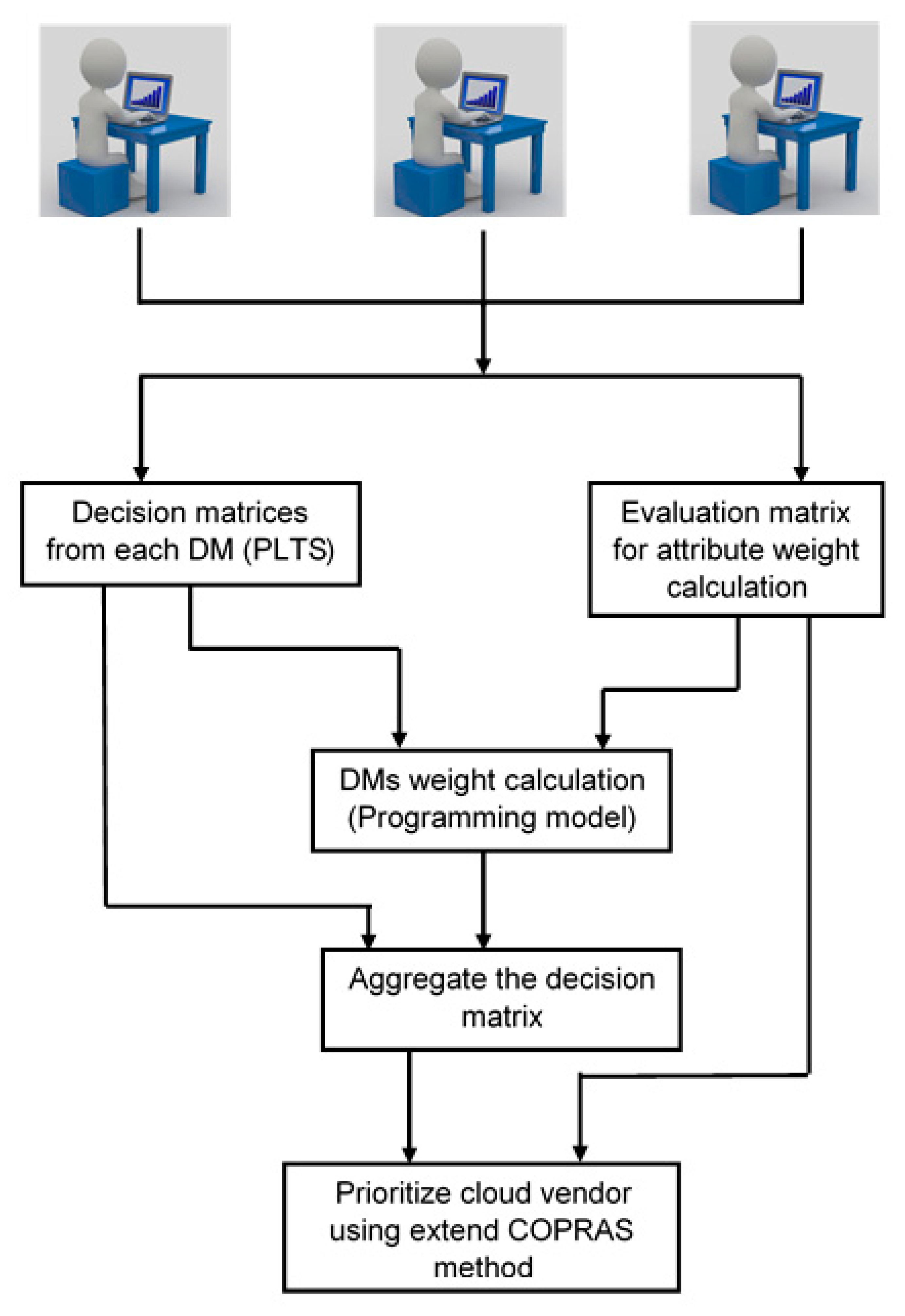
3. Proposed Decision Framework for CV Selection

Before presenting the core methods of the decision framework, it is substantial to discuss the specifics of the problem being addressed. There are $l$ DMs each forming a decision matrix of order $m\times n$, where $m$ is the number of CVs and $n$ is the number of attributes. The PLTS information is used for rating CVs over each attribute. Initially, the $l$ decision matrices of order $m\times n$ are aggregated to form a single decision matrix of order $m\times n$. During the process of aggregation, the interrelationship among attributes is considered effectively and weights of each DM are calculated in a systematic manner. Then, attributes’ weights are calculated by using a matrix of order $l\times n$. This is a vector of order $1\times n$, By using this vector and the aggregated matrix, a vector of order $1\times m$ is formed (from the ranking method) which is used for the prioritization of CVs.

3.1. Proposed Attributes’ Weight Calculation Method

This section puts forward a new method for calculating weights of attributes under PLTS context. The idea is to extend the SV method to PLTS. Previous weight calculation methods viz., analytical hierarchy process (AHP), optimization model, entropy measures, etc., suffer from the following weaknesses, such as, (i) complex implementation procedure, (ii) unreasonable weight values, and (iii) ineffective capturing of hesitation of DMs. To address the weaknesses, Liu et al. used the SV method for weight calculation, which enjoys the following advantages: (i) SV method is simple and easy to implement, (ii) produces reasonable weight values by focusing on all data points before determining the distribution, and (iii) captures hesitation effectively, by assigning high weights to those attributes, which cause confusion to DMs during preference elicitation.

Motivated by the strength of the SV method, in this paper, we extend the SV method to PLTS context. The procedure for calculating weights when the information about attributes is completely unknown is given below:

Step 1:

Form a weight calculation matrix with PLTS information of order $l\times n$ where $l$ denotes the number of DMs and $n$ denotes the number of attributes.

Step 2:

Transform the PLTS information into a single value matrix by using Equation (5).

$$sva{l}_{ij}={\displaystyle \sum }_{k=1}^{\#L\left(p\right)}{v}^k{p}^k$$

(5)

where $v^k$ is the $k^{th}$ subscript of the linguistic term, $\#L\left(p\right)$ is the total number of instances, and $p^k$ is the $k^{th}$ occurring probability associated with that linguistic term.

Step 3:

Determine the SV for each attribute by using Equation (6). The SV is a vector of order $1\times n$.

$${\sigma }_j^2=\frac{{{\displaystyle \sum }}_{l=1}^{\#DM}{\left(sva{l}_{lj}-\overline{sva{l}_j}\right)}^2}{\#DM-1}$$

(6)

where $\overline{sva{l}_j}$ is the mean value of the $j^{th}$ attribute, ${\sigma }_j^2$ is the SV of the $j^{th}$ attribute, and $\#DM$ is the total number of DMs.

Step 4:

Normalize the SV from step 3 to obtain weights of attributes. Use Equation (7) to obtain the weight vector of order $1\times n$.

$$w_j=\frac{{\sigma }_j^2}{{{\displaystyle \sum }}_j{\sigma }_j^2}$$

(7)

where $w_j$ is the weight of the $j^{th}$ attribute.

3.2. Proposed DMs’ Weight Calculation Method

This section proposes a new method for DMs’ weight calculation under PLTS context. Generally, DMs’ weight values are directly obtained, which causes inaccuracies in the decision-making process and are prone to imprecision, due to external factors like time, cost, environmental pressure, etc. [29]. Motivated by this issue, researchers started proposing methods for DMs’ weight calculation. Koksalmis and Kabak [30] conducted an attractive analysis of different methods for DMs’ weight calculation, and claimed that weights of DMs must be systematically calculated for reducing inaccuracies and imprecision in the decision-making process.

Motivated by this claim, in this paper, a new programming model is proposed for DMs’ weight calculation under PLTS context. To the best of our knowledge, this is the first study that calculates DMs’ weights with PLTS information. Moreover, in this paper, we make use of the partially known information about each DM to calculate the weights. Some advantages of the proposed method are: (i) it provides rational weight values, which reduce inaccuracies in the decision-making process and (ii) utilizes the partial information about each DM effectively to calculate weights. Attracted by these advantages, the procedure is presented below for DMs’ weight calculation.

Step 1:

Transform the decision matrix from each DM into weighted decision matrices by using Equation (8).

$$L\left(p\right)=\left\{v^k\left(1-{\left(1-p^k\right)}^{w_j}\right)\right\}$$

(8)

where $v^k$ is the subscript of the $k^{th}$ linguistic term, $p^k$ is the probability associated with the $k^{th}$ linguistic term, and $w_j$ is the weight of the $j^{th}$ attribute.

Equation (8) is applied to all the elements of the decision matrix from each DM. Now all matrices are transformed into weighted decision matrices.

Step 2:

Calculate positive ideal solution (PIS) and negative ideal solution (NIS) from the decision matrices obtained from step 1. The PIS and NIS values are calculated for each attribute, and it is given by Equations (9) and (10).

$$h^{+}=ma{x}_{j\in benefit}\left({\displaystyle \sum }_{k=1}^{\#L\left(p\right)}{v}^k{p}^k\right)ormi{n}_{j\in cost}\left({\displaystyle \sum }_{k=1}^{\#L\left(p\right)}{v}^k{p}^k\right)$$

(9)

$$h^{-}=ma{x}_{j\in cost}\left({\displaystyle \sum }_{k=1}^{\#L\left(p\right)}{v}^k{p}^k\right)ormi{n}_{j\in benefit}\left({\displaystyle \sum }_{k=1}^{\#L\left(p\right)}{v}^k{p}^k\right)$$

(10)

where $h^{+}$ is the PIS and $h^{-}$ is the NIS.

Equations (9) and (10) calculate PIS and NIS for each attribute and the PLTS information corresponding to the respective obtained value is considered for further process.

Step 3:

A programming model is proposed for determining weights of DMs. This model is solved using MATLAB^® optimization toolbox for calculating the weights of DMs.

Model 1.

$$MinZ={\displaystyle \sum }_{l=1}^{\#DM}d{w}_l{\displaystyle \sum }_{i=1}^m{\displaystyle \sum }_{j=1}^n\left(d\left(L_{ij}\left(p\right),h_j^{+}\right)-d\left(L_{ij}\left(p\right),h_j^{-}\right)\right)$$

Subject to

$$0\le d{w}_l\le 1$$

$${\displaystyle \sum }_{l}d{w}_l=1$$

Here$d\left(a,b\right)$is calculated using Equation (11) with$a$and$b$being any two PLEs.

$$d\left(a,b\right)=\sqrt{{\displaystyle \sum }_{k=1}^{\#L\left(p\right)}{\left(\left(v_a^k{p}_a^k\right)-\left(v_b^k{p}_b^k\right)\right)}^2}$$

(11)

Model 1 is solved by properly making use of the partial information about each DM which provides the weight for each DM.

3.3. Proposed Hybrid Aggregation Operator under PLTS Context

This section presents a hybrid aggregation operator for aggregating PLEs. The operator has two stages. In the first stage, the linguistic terms are aggregated, and in the second stage, the occurring probability values associated with each linguistic term are aggregated. A new procedure is proposed for aggregating the linguistic term. The MM operator is extended under the PLTS context for aggregating the occurring probability value associated with each linguistic term.

Previous aggregation operators under PLTS context do not capture the interrelationship among attributes and produce virtual sets. Motivated by this challenge and to address the same, in this paper, a hybrid operator is proposed, which captures the inter-relationship between attributes properly and avoids the formation of virtual sets.

Definition 5.

The aggregation of PLEs by using the proposed hybrid operator is a mapping$D^n\to D$, and it is given by,

$$Hybrid\left(v_1^k,v_2^k,\dots ,v_{\#DM}^k\right)=\left\{\begin{array}{c}condition1ifthefrequencyoflinguistictermoccurrenceisunique\\ condition2ifthefrequencyoflinguistictermoccurrenceisnotunique\end{array}\right\}$$

(12)

where condition 1 calculates the mean value of the linguistic term and then round-off is used to avoid virtual sets; condition 2 calculates the frequency of the linguistic term and the term with maximum frequency is chosen as aggregated value.

$$Hybrid\left(p_1^k,p_2^k,\dots ,p_{\#DM}^k\right)={\left({\displaystyle \prod }_{l=1}^{\#DM}{\left({\displaystyle \prod }_{q=1}^{\#DM}{\left(p_l^k\right)}^{{\lambda }_q}\right)}^{d{w}_l}\right)}^{\frac{1}{{{\displaystyle \sum }}_q{\lambda }_q}}$$

(13)

where$d{w}_l$is the weight of the$l^{th}$DM obtained fromSection 3.2,${\lambda }_1,{\lambda }_2,\dots ,{\lambda }_{\#DM}$are the risk appetite values associated with each DM which can have possible values from the set$\left\{1,2,\dots ,\#DM\right\}$.

Here Equation (12) is used to aggregate the linguistic term, and Equation (13) is used to aggregate the associated occurring probability values.

Property 1: Commutativity

If $L_l^{*}\left(p\right)\forall l=1,2,\dots ,\#DM$ is any permutation of PLEs then, $Hybrid\left(L_1^{*}\left(p\right),L_2^{*}\left(p\right),\dots ,L_{\#DM}^{*}\left(p\right)\right)=Hybrid\left(L_1\left(p\right),L_2\left(p\right),\dots ,L_{\#DM}\left(p\right)\right)$.

Property 2: Bounded

If $L_i\left(p\right)\forall l=1,2,\dots ,\#DM$ is a collection of PLEs then, $L^{-}\left(p\right)\le Hybrid\left(L_1\left(p\right),L_2\left(p\right),\dots ,L_{\#DM}\left(p\right)\right)\le L^{+}\left(p\right)$. Here, $L^{-}\left(p\right)=mi{n}_i\left({\displaystyle \sum }_{k=1}^{\#L_i\left(p\right)}\left(v_i^k{p}_i^k\right)\right)$ and $L^{-}\left(p\right)=ma{x}_i\left({\displaystyle \sum }_{k=1}^{\#L_i\left(p\right)}\left(v_i^k{p}_i^k\right)\right)$.

Property 3: Idempotent

If $L_1\left(p\right),L_2\left(p\right),\dots ,L_{\#DM}\left(p\right)=L\left(p\right)$ then, $Hybrid\left(L_1\left(p\right),L_2\left(p\right),\dots ,L_{\#DM}\left(p\right)\right)=L\left(p\right)$.

Property 4: Monotonicity

Consider a set of PLEs $L_l^{*}\left(p\right)\forall l=1,2,\dots ,\#DM$ such that $L_l^{*}\left(p\right)\ge L_i\left(p\right)\forall l=1,2,\dots ,\#DM$ then, $Hybrid\left(L_1^{*}\left(p\right),L_2^{*}\left(p\right),\dots ,L_{\#DM}^{*}\left(p\right)\right)\ge Hybrid\left(L_1\left(p\right),L_2\left(p\right),\dots ,L_{\#DM}\left(p\right)\right)$.

Theorem 1.

The aggregation of PLEs by using the proposed hybrid operator produces a PLE.

Proof. 

The proposed hybrid operator aggregates PLEs in two stages. In the first stage, linguistic terms are aggregated, and in the second stage, the associated occurring probability values are aggregated. Clearly, from Equation (12), no virtual element is obtained and hence, the linguistic information is rationally aggregated. Now, we must prove that the aggregation of associated occurring probability value yields a probability value. For this, we make use of the Bounded property. This property shows that the aggregated value is bounded within the lower and upper limits. By extending the property, we get $0\le {\left({\displaystyle \prod }_{l=1}^{\#DM}{\left({\displaystyle \prod }_{q=1}^{\#DM}{\left(p_l^k\right)}^{{\lambda }_q}\right)}^{d{w}_l}\right)}^{\frac{1}{{{\displaystyle \sum }}_q{\lambda }_q}}\le 1$.

Thus, $0\le Hybrid\left(p_1^k,p_2^k,\dots ,p_{\#DM}^k\right)\le 1$ holds true. By combining the idea, we can infer that the aggregation produces a PLE. □

Some advantages of the proposed hybrid operator are:

• Formation of a virtual set is avoided.
• The inter-relationships between attributes is properly captured.
• Risk appetite values are considered along with the relative importance of each DM.
• The relative importance of each DM is calculated systematically by properly capturing the uncertainty in the process.

3.4. Extended COPRAS Method Under PLTS Context

This section puts forward a new extension to the COPRAS method under PLTS context. The initial idea for COPRAS method was obtained from [31] and Zavadskas et al. [32] analyzed different MAGDM methods, and described the importance of COPRAS method, in solving decision-making problems. COPRAS is a simple and straightforward method for ranking alternatives. It captures the direct and proportional relationship between alternatives and attributes with significance and utility degrees. Further, the COPRAS method could provide ranking from different angles, which promote rational decision-making [31].

Motivated by these strengths, researchers used the COPRAS method for various decision-making problems. Zavadskas et al. [33,34] used the COPRAS method, with grey numbers for ranking project managers and contractors. Vahdani et al. [35] and Gorabe et al. [36] used the COPRAS method for robot selection in industries. Chatterjee et al. [37,38] and Nasab et al. [39] extended the COPRAS method for material selection. Chatterjee and Kar [40] extended COPRAS for Z-numbers and applied the same for renewable energy source selection. Yazdani et al. [41] presented a hybrid method for the green supplier selection by combining quality function deployment (QFD) and the COPRAS method.

From the analysis made above, it can be inferred that the COPRAS method is powerful for prioritization of alternatives and its extension to PLTS context is not developed so far. Motivated by the advantages of the COPRAS method, in this paper, the COPRAS method is extended for PLTS context. The systematic procedure is given below:

Step 1:

Identify the benefit and cost type attributes. The aggregated matrix from Section 3.3 (of order $m\times n$) and the attributes’ weight vector (of order $1\times n$) from Section 3.1 is considered as input for the prioritization process.

Step 2:

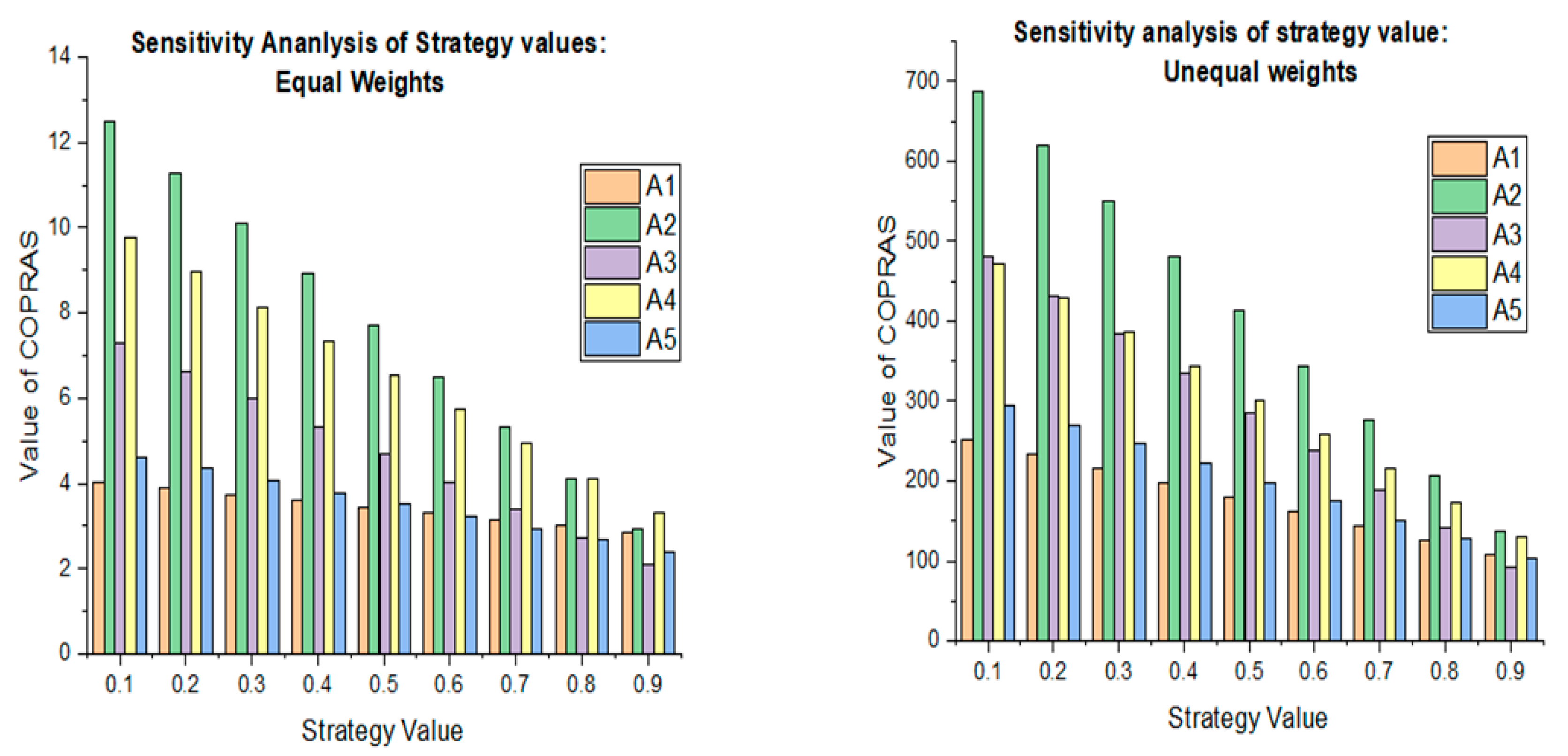
Calculate the COPRAS parameters by using Equations (14) and (15). These parameters are calculated for each alternative under both equal and unequal attributes’ weight conditions.

$$P_i={⨁}_{j=1}^z{w}_j{v}_{ij}^k\times {⨁}_{j=1}^{z}1-{\left(1-p_{ij}^k\right)}^{w_j}$$

(14)

$$R_i={⨁}_{j=1}^{z+1}{w}_j{v}_{ij}^k\times {⨁}_{j=1}^{z+1}1-{\left(1-p_{ij}^k\right)}^{w_j}$$

(15)

Step 3:

Determine the prioritization order by using Equation (16). This parameter is also calculated for each alternative.

$$Q_i=\phi P_i+\left(1-\phi \right)\frac{{{\displaystyle \sum }}_i{R}_i}{R_i\left(\frac{1}{{{\displaystyle \sum }}_i{R}_i}\right)}$$

(16)

where $\phi$ is the strategy value in the range 0 to 1.

Before demonstrating the numerical example of CV selection, it is better to present the diagrammatic representation of the decision framework to clearly understand the working of the proposed decision framework (refer Figure 1 for clarity).

Figure 1 depicts the overall workflow of the proposed decision framework for CV selection. The framework is used to initially determine the weights of the attributes. Then, the DMs’ weights are determined, and the preferences are aggregated, using these weight vectors. Further, the CVs are prioritized by using a ranking method under PLTS context. The aggregated matrix and the attributes’ weight values are taken as input for prioritization. Finally, the proposed framework is validated by using a numerical example which is presented below.

4. Numerical Example of Cloud Vendor Selection

This section demonstrates the practical use of the proposed framework by prioritizing CVs. An organization in Chennai wants to attain global standards, and so they think of migrating their infrastructural needs to cloud. This brings enough time and resources for planning the core developmental activities. For achieving the desired objective, the board decides to constitute a panel of three DMs including., senior technical officer $d_1$, audit and finance personnel $d_2$ and senior computer engineer $d_3$ who provide their preferences over each CV for a specific attribute.

The panel analyzes different CVs who offer IaaS, and by adopting the Delphi method, they picked 13 CVs for analysis. By the process of repeated discussion and brainstorming, the panel finalized five CVs (A1, A2, A3, A4, A5) who actively offer IaaS. Then, the DMs made a literature analysis, and by the method of voting, six attributes were chosen for analysis. These six attributes (C1, C2, C3, C4, C5, C6) were chosen after a detailed discussion and analysis of various benchmark standards being, information communication technology service quality (ICTSQ), application performance index (APDEX), service measurement index (SMI) and ISO/IEC 9126 [42]. Along with these benchmarks, some literature reviews are also analyzed for obtaining proper attributes for evaluation. All attributes were listed and based on the scoring method, six attributes are finalized, and they are accountability, assurance, agility, performance, cost, and risk of CV.

The systematic procedure for the proposed decision framework is given below:

Step 1:

Start.

Step 2:

Form three decision matrices of order $5\times 6$ where five CVs are rated by using six attributes. The DMs use PLTS information for preference elicitation.

Table 2. PLTS information provided by $d_1$

Decision Maker-1
CSPs	C1	C2	C3	C4	C5	C6
A1	$\left\{\begin{array}{c}{s}_1\left(0.44\right)\\ s_3\left(0.34\right)\end{array}\right\}$	$\left\{\begin{array}{c}{s}_1\left(023\right)\\ s_2\left(0.49\right)\end{array}\right\}$	$\left\{\begin{array}{c}{s}_1\left(0.32\right)\\ s_5\left(0.19\right)\end{array}\right\}$	$\left\{\begin{array}{c}{s}_1\left(0.48\right)\\ s_3\left(0.12\right)\end{array}\right\}$	$\left\{\begin{array}{c}{s}_3\left(0.38\right)\\ s_2\left(0.58\right)\end{array}\right\}$	$\left\{\begin{array}{c}{s}_2\left(0.62\right)\\ s_2\left(0.27\right)\end{array}\right\}$
A2	$\left\{\begin{array}{c}{s}_5\left(0.37\right)\\ s_5\left(0.17\right)\end{array}\right\}$	$\left\{\begin{array}{c}{s}_3\left(0.46\right)\\ s_1\left(0.44\right)\end{array}\right\}$	$\left\{\begin{array}{c}{s}_5\left(0.59\right)\\ s_2\left(0.02\right)\end{array}\right\}$	$\left\{\begin{array}{c}{s}_3\left(0.16\right)\\ s_2\left(0.18\right)\end{array}\right\}$	$\left\{\begin{array}{c}{s}_3\left(0.30\right)\\ s_1\left(0.24\right)\end{array}\right\}$	$\left\{\begin{array}{c}{s}_4\left(0.64\right)\\ s_4\left(0.03\right)\end{array}\right\}$
A3	$\left\{\begin{array}{c}{s}_1\left(0.27\right)\\ s_2\left(0.33\right)\end{array}\right\}$	$\left\{\begin{array}{c}{s}_3\left(0.36\right)\\ s_5\left(0.49\right)\end{array}\right\}$	$\left\{\begin{array}{c}{s}_3\left(0.11\right)\\ s_2\left(0.61\right)\end{array}\right\}$	$\left\{\begin{array}{c}{s}_4\left(0.09\right)\\ s_3\left(0.27\right)\end{array}\right\}$	$\left\{\begin{array}{c}{s}_1\left(0.44\right)\\ s_2\left(0.53\right)\end{array}\right\}$	$\left\{\begin{array}{c}{s}_3\left(0.26\right)\\ s_5\left(0.47\right)\end{array}\right\}$
A4	$\left\{\begin{array}{c}{s}_4\left(0.24\right)\\ s_5\left(0.68\right)\end{array}\right\}$	$\left\{\begin{array}{c}{s}_2\left(0.70\right)\\ s_4\left(0.07\right)\end{array}\right\}$	$\left\{\begin{array}{c}{s}_2\left(0.34\right)\\ s_2\left(0.42\right)\end{array}\right\}$	$\left\{\begin{array}{c}{s}_2\left(0.68\right)\\ s_4\left(0.01\right)\end{array}\right\}$	$\left\{\begin{array}{c}{s}_4\left(0.80\right)\\ s_2\left(0.15\right)\end{array}\right\}$	$\left\{\begin{array}{c}{s}_3\left(0.23\right)\\ s_3\left(0.39\right)\end{array}\right\}$
A5	$\left\{\begin{array}{c}{s}_2\left(0.47\right)\\ s_4\left(0.04\right)\end{array}\right\}$	$\left\{\begin{array}{c}{s}_1\left(0.47\right)\\ s_4\left(0.15\right)\end{array}\right\}$	$\left\{\begin{array}{c}{s}_2\left(0.19\right)\\ s_4\left(0.74\right)\end{array}\right\}$	$\left\{\begin{array}{c}{s}_2\left(0.14\right)\\ s_5\left(0.39\right)\end{array}\right\}$	$\left\{\begin{array}{c}{s}_1\left(0.09\right)\\ s_2\left(0.58\right)\end{array}\right\}$	$\left\{\begin{array}{c}{s}_4\left(0.22\right)\\ s_3\left(0.32\right)\end{array}\right\}$
Decision Maker-2
A1	$\left\{\begin{array}{c}{s}_4\left(0.32\right)\\ s_4\left(0.48\right)\end{array}\right\}$	$\left\{\begin{array}{c}{s}_2\left(0.24\right)\\ s_4\left(0.12\right)\end{array}\right\}$	$\left\{\begin{array}{c}{s}_4\left(0.23\right)\\ s_3\left(0.33\right)\end{array}\right\}$	$\left\{\begin{array}{c}{s}_4\left(0.33\right)\\ s_2\left(0.21\right)\end{array}\right\}$	$\left\{\begin{array}{c}{s}_5\left(0.26\right)\\ s_5\left(0.61\right)\end{array}\right\}$	$\left\{\begin{array}{c}{s}_3\left(0.44\right)\\ s_3\left(0.13\right)\end{array}\right\}$
A2	$\left\{\begin{array}{c}{s}_2\left(0.47\right)\\ s_1\left(0.33\right)\end{array}\right\}$	$\left\{\begin{array}{c}{s}_3\left(0.27\right)\\ s_4\left(0.33\right)\end{array}\right\}$	$\left\{\begin{array}{c}{s}_3\left(0.26\right)\\ s_4\left(0.50\right)\end{array}\right\}$	$\left\{\begin{array}{c}{s}_2\left(0.11\right)\\ s_1\left(0.06\right)\end{array}\right\}$	$\left\{\begin{array}{c}{s}_3\left(0.19\right)\\ s_3\left(0.38\right)\end{array}\right\}$	$\left\{\begin{array}{c}{s}_4\left(0.47\right)\\ s_4\left(0.49\right)\end{array}\right\}$
A3	$\left\{\begin{array}{c}{s}_1\left(0.70\right)\\ s_1\left(0.09\right)\end{array}\right\}$	$\left\{\begin{array}{c}{s}_3\left(0.43\right)\\ s_3\left(0.24\right)\end{array}\right\}$	$\left\{\begin{array}{c}{s}_2\left(0.37\right)\\ s_4\left(0.26\right)\end{array}\right\}$	$\left\{\begin{array}{c}{s}_2\left(0.59\right)\\ s_1\left(0.26\right)\end{array}\right\}$	$\left\{\begin{array}{c}{s}_1\left(0.24\right)\\ s_4\left(0.44\right)\end{array}\right\}$	$\left\{\begin{array}{c}{s}_4\left(0.37\right)\\ s_2\left(0.20\right)\end{array}\right\}$
A4	$\left\{\begin{array}{c}{s}_4\left(0.44\right)\\ s_4\left(0.02\right)\end{array}\right\}$	$\left\{\begin{array}{c}{s}_2\left(0.27\right)\\ s_3\left(0.20\right)\end{array}\right\}$	$\left\{\begin{array}{c}{s}_5\left(0.45\right)\\ s_3\left(0.20\right)\end{array}\right\}$	$\left\{\begin{array}{c}{s}_4\left(0.41\right)\\ s_2\left(0.38\right)\end{array}\right\}$	$\left\{\begin{array}{c}{s}_2\left(0.40\right)\\ s_2\left(0.48\right)\end{array}\right\}$	$\left\{\begin{array}{c}{s}_2\left(0.22\right)\\ s_4\left(0.42\right)\end{array}\right\}$
A5	$\left\{\begin{array}{c}{s}_4\left(0.43\right)\\ s_1\left(0.50\right)\end{array}\right\}$	$\left\{\begin{array}{c}{s}_3\left(0.59\right)\\ s_5\left(0.15\right)\end{array}\right\}$	$\left\{\begin{array}{c}{s}_1\left(0.38\right)\\ s_3\left(0.42\right)\end{array}\right\}$	$\left\{\begin{array}{c}{s}_4\left(0.53\right)\\ s_2\left(0.09\right)\end{array}\right\}$	$\left\{\begin{array}{c}{s}_1\left(0.34\right)\\ s_1\left(0.25\right)\end{array}\right\}$	$\left\{\begin{array}{c}{s}_1\left(0.15\right)\\ s_3\left(0.05\right)\end{array}\right\}$
Decision Maker-3
A1	$\left\{\begin{array}{c}{s}_5\left(0.47\right)\\ s_3\left(0.35\right)\end{array}\right\}$	$\left\{\begin{array}{c}{s}_3\left(0.44\right)\\ s_5\left(0.50\right)\end{array}\right\}$	$\left\{\begin{array}{c}{s}_1\left(0.31\right)\\ s_5\left(0.50\right)\end{array}\right\}$	$\left\{\begin{array}{c}{s}_3\left(0.40\right)\\ s_3\left(0.12\right)\end{array}\right\}$	$\left\{\begin{array}{c}{s}_3\left(0.29\right)\\ s_5\left(0.43\right)\end{array}\right\}$	$\left\{\begin{array}{c}{s}_4\left(0.25\right)\\ s_3\left(0.67\right)\end{array}\right\}$
A2	$\left\{\begin{array}{c}{s}_1\left(0.33\right)\\ s_4\left(0.37\right)\end{array}\right\}$	$\left\{\begin{array}{c}{s}_5\left(0.39\right)\\ s_5\left(0.29\right)\end{array}\right\}$	$\left\{\begin{array}{c}{s}_5\left(0.02\right)\\ s_3\left(0.12\right)\end{array}\right\}$	$\left\{\begin{array}{c}{s}_5\left(0.42\right)\\ s_3\left(0.11\right)\end{array}\right\}$	$\left\{\begin{array}{c}{s}_3\left(0.03\right)\\ s_4\left(0.61\right)\end{array}\right\}$	$\left\{\begin{array}{c}{s}_2\left(0.49\right)\\ s_1\left(0.19\right)\end{array}\right\}$
A3	$\left\{\begin{array}{c}{s}_1\left(0.15\right)\\ s_2\left(0.19\right)\end{array}\right\}$	$\left\{\begin{array}{c}{s}_1\left(0.28\right)\\ s_4\left(0.54\right)\end{array}\right\}$	$\left\{\begin{array}{c}{s}_4\left(0.54\right)\\ s_3\left(0.45\right)\end{array}\right\}$	$\left\{\begin{array}{c}{s}_1\left(0.43\right)\\ s_3\left(0.44\right)\end{array}\right\}$	$\left\{\begin{array}{c}{s}_2\left(0.28\right)\\ s_2\left(0.32\right)\end{array}\right\}$	$\left\{\begin{array}{c}{s}_3\left(0.48\right)\\ s_2\left(0.04\right)\end{array}\right\}$
A4	$\left\{\begin{array}{c}{s}_1\left(0.17\right)\\ s_1\left(0.62\right)\end{array}\right\}$	$\left\{\begin{array}{c}{s}_3\left(0.47\right)\\ s_1\left(0.37\right)\end{array}\right\}$	$\left\{\begin{array}{c}{s}_4\left(0.43\right)\\ s_1\left(0.47\right)\end{array}\right\}$	$\left\{\begin{array}{c}{s}_5\left(0.40\right)\\ s_5\left(0.26\right)\end{array}\right\}$	$\left\{\begin{array}{c}{s}_1\left(0.13\right)\\ s_2\left(0.03\right)\end{array}\right\}$	$\left\{\begin{array}{c}{s}_5\left(0.30\right)\\ s_2\left(0.33\right)\end{array}\right\}$
A5	$\left\{\begin{array}{c}{s}_3\left(0.03\right)\\ s_4\left(0.84\right)\end{array}\right\}$	$\left\{\begin{array}{c}{s}_3\left(0.35\right)\\ s_5\left(0.45\right)\end{array}\right\}$	$\left\{\begin{array}{c}{s}_1\left(0.66\right)\\ s_1\left(0.33\right)\end{array}\right\}$	$\left\{\begin{array}{c}{s}_5\left(0.50\right)\\ s_1\left(0.27\right)\end{array}\right\}$	$\left\{\begin{array}{c}{s}_4\left(0.29\right)\\ s_5\left(0.41\right)\end{array}\right\}$	$\left\{\begin{array}{c}{s}_3\left(0.82\right)\\ s_4\left(0.10\right)\end{array}\right\}$

depicts the PLTS information provided by each DM for rating CVs over a specific attribute. Each DM uses two instances to rate the CVs, and they associate an occurring probability value for each linguistic term. The LTS used for analysis is a 5-Likert rating scale given by $S=\left\{s_o=verylow,s_1=low,s_2=medium,s_3=high,s_4=veryhigh\right\}$.

Step 3:

Form an attribute weight calculation matrix of order $3\times 6$ where three DMs provide their preferences on each of the six attributes.

Table 3. Attributes weight calculation matrix.

DMs	C1	C2	C3	C4	C5	C6
D1	$\left\{\begin{array}{c}{s}_2\left(0.35\right)\\ s_1\left(0.12\right)\end{array}\right\}$	$\left\{\begin{array}{c}{s}_5\left(0.47\right)\\ s_1\left(0.20\right)\end{array}\right\}$	$\left\{\begin{array}{c}{s}_1\left(0.37\right)\\ s_2\left(0.40\right)\end{array}\right\}$	$\left\{\begin{array}{c}{s}_3\left(0.89\right)\\ s_4\left(0.05\right)\end{array}\right\}$	$\left\{\begin{array}{c}{s}_2\left(0.20\right)\\ s_1\left(0.72\right)\end{array}\right\}$	$\left\{\begin{array}{c}{s}_4\left(0.58\right)\\ s_5\left(0.07\right)\end{array}\right\}$
D2	$\left\{\begin{array}{c}{s}_5\left(0.29\right)\\ s_5\left(0.54\right)\end{array}\right\}$	$\left\{\begin{array}{c}{s}_5\left(0.42\right)\\ s_4\left(0.22\right)\end{array}\right\}$	$\left\{\begin{array}{c}{s}_3\left(0.14\right)\\ s_3\left(0.38\right)\end{array}\right\}$	$\left\{\begin{array}{c}{s}_3\left(0.31\right)\\ s_4\left(0.14\right)\end{array}\right\}$	$\left\{\begin{array}{c}{s}_3\left(0.40\right)\\ s_2\left(0.39\right)\end{array}\right\}$	$\left\{\begin{array}{c}{s}_4\left(0.02\right)\\ s_1\left(0.56\right)\end{array}\right\}$
D3	$\left\{\begin{array}{c}{s}_2\left(0.49\right)\\ s_5\left(0.15\right)\end{array}\right\}$	$\left\{\begin{array}{c}{s}_5\left(0.30\right)\\ s_5\left(0.44\right)\end{array}\right\}$	$\left\{\begin{array}{c}{s}_5\left(0.37\right)\\ s_3\left(0.29\right)\end{array}\right\}$	$\left\{\begin{array}{c}{s}_1\left(0.33\right)\\ s_3\left(0.26\right)\end{array}\right\}$	$\left\{\begin{array}{c}{s}_2\left(0.42\right)\\ s_5\left(0.43\right)\end{array}\right\}$	$\left\{\begin{array}{c}{s}_2\left(0.44\right)\\ s_3\left(0.47\right)\end{array}\right\}$

presents the evaluation matrix for calculating attributes’ weights. Each DM provides his/her preference over each attribute and using these preferences, the attributes’ weights are calculated by using the procedure given in Section 3.1. The mean value for each attribute is given by (2.23, 3.08, 1.82, 1.82, 2.03, 1.16) and the variance value for each attribute is given by (2.96, 0.34, 0.65, 0.86, 0.88, 1.16). By normalizing the variance, we get the weight of values as (0.17, 0.24, 0.14, 0.14, 0.16, 0.15).

Step 4:

Aggregate the three decision matrices by using the proposed aggregation operator (refer Section 3.3). The operator uses DMs’ weights calculated from Section 3.2 for aggregation.

Table 4. Weighted PLTS information of decision makers.

Decision Maker-1
CSPs	C1	C2	C3	C4	C5	C6
A1	$\left\{\begin{array}{c}{s}_1\left(0.82\right)\\ s_3\left(0.71\right)\end{array}\right\}$	$\left\{\begin{array}{c}{s}_1\left(0.09\right)\\ s_2\left(0.20\right)\end{array}\right\}$	$\left\{\begin{array}{c}{s}_1\left(0.22\right)\\ s_5\left(0.13\right)\end{array}\right\}$	$\left\{\begin{array}{c}{s}_1\left(0.43\right)\\ s_3\left(0.10\right)\end{array}\right\}$	$\left\{\begin{array}{c}{s}_3\left(0.34\right)\\ s_2\left(0.53\right)\end{array}\right\}$	$\left\{\begin{array}{c}{s}_2\left(0.68\right)\\ s_2\left(0.31\right)\end{array}\right\}$
A2	$\left\{\begin{array}{c}{s}_5\left(0.75\right)\\ s_5\left(0.42\right)\end{array}\right\}$	$\left\{\begin{array}{c}{s}_3\left(0.19\right)\\ s_1\left(0.18\right)\end{array}\right\}$	$\left\{\begin{array}{c}{s}_5\left(0.44\right)\\ s_2\left(0.01\right)\end{array}\right\}$	$\left\{\begin{array}{c}{s}_3\left(0.14\right)\\ s_2\left(0.16\right)\end{array}\right\}$	$\left\{\begin{array}{c}{s}_3\left(0.27\right)\\ s_1\left(0.21\right)\end{array}\right\}$	$\left\{\begin{array}{c}{s}_4\left(0.70\right)\\ s_4\left(0.04\right)\end{array}\right\}$
A3	$\left\{\begin{array}{c}{s}_1\left(0.61\right)\\ s_2\left(0.69\right)\end{array}\right\}$	$\left\{\begin{array}{c}{s}_3\left(0.14\right)\\ s_5\left(0.20\right)\end{array}\right\}$	$\left\{\begin{array}{c}{s}_3\left(0.07\right)\\ s_2\left(0.46\right)\end{array}\right\}$	$\left\{\begin{array}{c}{s}_4\left(0.08\right)\\ s_3\left(0.24\right)\end{array}\right\}$	$\left\{\begin{array}{c}{s}_1\left(0.40\right)\\ s_2\left(0.49\right)\end{array}\right\}$	$\left\{\begin{array}{c}{s}_3\left(0.30\right)\\ s_5\left(0.52\right)\end{array}\right\}$
A4	$\left\{\begin{array}{c}{s}_4\left(0.56\right)\\ s_5\left(0.97\right)\end{array}\right\}$	$\left\{\begin{array}{c}{s}_2\left(0.34\right)\\ s_4\left(0.02\right)\end{array}\right\}$	$\left\{\begin{array}{c}{s}_2\left(0.24\right)\\ s_2\left(0.30\right)\end{array}\right\}$	$\left\{\begin{array}{c}{s}_2\left(0.62\right)\\ s_4\left(0.01\right)\end{array}\right\}$	$\left\{\begin{array}{c}{s}_4\left(0.76\right)\\ s_2\left(0.13\right)\end{array}\right\}$	$\left\{\begin{array}{c}{s}_3\left(0.26\right)\\ s_3\left(0.44\right)\end{array}\right\}$
A5	$\left\{\begin{array}{c}{s}_2\left(0.85\right)\\ s_4\left(0.11\right)\end{array}\right\}$	$\left\{\begin{array}{c}{s}_1\left(0.19\right)\\ s_4\left(0.05\right)\end{array}\right\}$	$\left\{\begin{array}{c}{s}_2\left(0.13\right)\\ s_4\left(0.58\right)\end{array}\right\}$	$\left\{\begin{array}{c}{s}_2\left(0.12\right)\\ s_5\left(0.35\right)\end{array}\right\}$	$\left\{\begin{array}{c}{s}_1\left(0.08\right)\\ s_2\left(0.53\right)\end{array}\right\}$	$\left\{\begin{array}{c}{s}_4\left(0.25\right)\\ s_3\left(0.36\right)\end{array}\right\}$
Decision Maker-2
A1	$\left\{\begin{array}{c}{s}_4\left(0.68\right)\\ s_4\left(0.86\right)\end{array}\right\}$	$\left\{\begin{array}{c}{s}_2\left(0.09\right)\\ s_4\left(0.04\right)\end{array}\right\}$	$\left\{\begin{array}{c}{s}_4\left(0.16\right)\\ s_3\left(0.23\right)\end{array}\right\}$	$\left\{\begin{array}{c}{s}_4\left(0.29\right)\\ s_2\left(0.18\right)\end{array}\right\}$	$\left\{\begin{array}{c}{s}_5\left(0.23\right)\\ s_5\left(0.56\right)\end{array}\right\}$	$\left\{\begin{array}{c}{s}_3\left(0.49\right)\\ s_3\left(0.15\right)\end{array}\right\}$
A2	$\left\{\begin{array}{c}{s}_2\left(0.85\right)\\ s_1\left(0.69\right)\end{array}\right\}$	$\left\{\begin{array}{c}{s}_3\left(0.10\right)\\ s_4\left(0.13\right)\end{array}\right\}$	$\left\{\begin{array}{c}{s}_3\left(0.18\right)\\ s_4\left(0.36\right)\end{array}\right\}$	$\left\{\begin{array}{c}{s}_2\left(0.10\right)\\ s_1\left(0.05\right)\end{array}\right\}$	$\left\{\begin{array}{c}{s}_3\left(0.17\right)\\ s_3\left(0.34\right)\end{array}\right\}$	$\left\{\begin{array}{c}{s}_4\left(0.52\right)\\ s_4\left(0.55\right)\end{array}\right\}$
A3	$\left\{\begin{array}{c}{s}_1\left(0.97\right)\\ s_1\left(0.24\right)\end{array}\right\}$	$\left\{\begin{array}{c}{s}_3\left(0.17\right)\\ s_3\left(0.09\right)\end{array}\right\}$	$\left\{\begin{array}{c}{s}_2\left(0.26\right)\\ s_4\left(0.18\right)\end{array}\right\}$	$\left\{\begin{array}{c}{s}_2\left(0.55\right)\\ s_1\left(0.23\right)\end{array}\right\}$	$\left\{\begin{array}{c}{s}_1\left(0.21\right)\\ s_4\left(0.40\right)\end{array}\right\}$	$\left\{\begin{array}{c}{s}_4\left(0.42\right)\\ s_2\left(0.23\right)\end{array}\right\}$
A4	$\left\{\begin{array}{c}{s}_4\left(0.82\right)\\ s_4\left(0.06\right)\end{array}\right\}$	$\left\{\begin{array}{c}{s}_2\left(0.10\right)\\ s_3\left(0.07\right)\end{array}\right\}$	$\left\{\begin{array}{c}{s}_5\left(0.32\right)\\ s_3\left(0.14\right)\end{array}\right\}$	$\left\{\begin{array}{c}{s}_4\left(0.36\right)\\ s_2\left(0.34\right)\end{array}\right\}$	$\left\{\begin{array}{c}{s}_2\left(0.36\right)\\ s_2\left(0.44\right)\end{array}\right\}$	$\left\{\begin{array}{c}{s}_2\left(0.25\right)\\ s_4\left(0.47\right)\end{array}\right\}$
A5	$\left\{\begin{array}{c}{s}_4\left(0.81\right)\\ s_1\left(0.87\right)\end{array}\right\}$	$\left\{\begin{array}{c}{s}_3\left(0.26\right)\\ s_5\left(0.05\right)\end{array}\right\}$	$\left\{\begin{array}{c}{s}_1\left(0.27\right)\\ s_3\left(0.30\right)\end{array}\right\}$	$\left\{\begin{array}{c}{s}_4\left(0.48\right)\\ s_2\left(0.08\right)\end{array}\right\}$	$\left\{\begin{array}{c}{s}_1\left(0.31\right)\\ s_1\left(0.22\right)\end{array}\right\}$	$\left\{\begin{array}{c}{s}_1\left(0.17\right)\\ s_3\left(0.06\right)\end{array}\right\}$
Decision Maker-3
A1	$\left\{\begin{array}{c}{s}_5\left(0.85\right)\\ s_3\left(0.72\right)\end{array}\right\}$	$\left\{\begin{array}{c}{s}_3\left(0.18\right)\\ s_5\left(0.21\right)\end{array}\right\}$	$\left\{\begin{array}{c}{s}_1\left(0.21\right)\\ s_5\left(0.36\right)\end{array}\right\}$	$\left\{\begin{array}{c}{s}_3\left(0.36\right)\\ s_3\left(0.10\right)\end{array}\right\}$	$\left\{\begin{array}{c}{s}_3\left(0.26\right)\\ s_5\left(0.39\right)\end{array}\right\}$	$\left\{\begin{array}{c}{s}_4\left(0.29\right)\\ s_3\left(0.73\right)\end{array}\right\}$
A2	$\left\{\begin{array}{c}{s}_1\left(0.69\right)\\ s_4\left(0.75\right)\end{array}\right\}$	$\left\{\begin{array}{c}{s}_5\left(0.15\right)\\ s_5\left(0.11\right)\end{array}\right\}$	$\left\{\begin{array}{c}{s}_5\left(0.01\right)\\ s_3\left(0.08\right)\end{array}\right\}$	$\left\{\begin{array}{c}{s}_5\left(0.37\right)\\ s_3\left(0.10\right)\end{array}\right\}$	$\left\{\begin{array}{c}{s}_3\left(0.03\right)\\ s_4\left(0.56\right)\end{array}\right\}$	$\left\{\begin{array}{c}{s}_2\left(0.55\right)\\ s_1\left(0.22\right)\end{array}\right\}$
A3	$\left\{\begin{array}{c}{s}_1\left(0.38\right)\\ s_2\left(0.46\right)\end{array}\right\}$	$\left\{\begin{array}{c}{s}_1\left(0.11\right)\\ s_4\left(0.23\right)\end{array}\right\}$	$\left\{\begin{array}{c}{s}_4\left(0.40\right)\\ s_3\left(0.32\right)\end{array}\right\}$	$\left\{\begin{array}{c}{s}_1\left(0.38\right)\\ s_3\left(0.39\right)\end{array}\right\}$	$\left\{\begin{array}{c}{s}_2\left(0.25\right)\\ s_2\left(0.29\right)\end{array}\right\}$	$\left\{\begin{array}{c}{s}_3\left(0.53\right)\\ s_2\left(0.05\right)\end{array}\right\}$
A4	$\left\{\begin{array}{c}{s}_1\left(0.42\right)\\ s_1\left(0.94\right)\end{array}\right\}$	$\left\{\begin{array}{c}{s}_3\left(0.19\right)\\ s_1\left(0.15\right)\end{array}\right\}$	$\left\{\begin{array}{c}{s}_4\left(0.31\right)\\ s_1\left(0.34\right)\end{array}\right\}$	$\left\{\begin{array}{c}{s}_5\left(0.36\right)\\ s_5\left(0.23\right)\end{array}\right\}$	$\left\{\begin{array}{c}{s}_1\left(0.12\right)\\ s_2\left(0.03\right)\end{array}\right\}$	$\left\{\begin{array}{c}{s}_5\left(0.34\right)\\ s_2\left(0.37\right)\end{array}\right\}$
A5	$\left\{\begin{array}{c}{s}_3\left(0.09\right)\\ s_4\left(1.00\right)\end{array}\right\}$	$\left\{\begin{array}{c}{s}_3\left(0.14\right)\\ s_5\left(0.18\right)\end{array}\right\}$	$\left\{\begin{array}{c}{s}_1\left(0.50\right)\\ s_1\left(0.23\right)\end{array}\right\}$	$\left\{\begin{array}{c}{s}_5\left(0.45\right)\\ s_1\left(0.24\right)\end{array}\right\}$	$\left\{\begin{array}{c}{s}_4\left(0.26\right)\\ s_5\left(0.37\right)\end{array}\right\}$	$\left\{\begin{array}{c}{s}_3\left(0.87\right)\\ s_4\left(0.12\right)\end{array}\right\}$

depicts the weighted preference information of each DM which is obtained by using Equation (8). These values are used for calculating the PIS and NIS values for each attribute, and they are shown in

Table 5. Ideal solution for each attribute from decision makers’ matrix.

Decision Maker-1
CSPs	C1	C2	C3	C4	C5	C6
PIS	$\left\{\begin{array}{c}{s}_4\left(0.56\right)\\ s_5\left(0.97\right)\end{array}\right\}$	$\left\{\begin{array}{c}{s}_3\left(0.14\right)\\ s_5\left(0.20\right)\end{array}\right\}$	$\left\{\begin{array}{c}{s}_2\left(0.13\right)\\ s_4\left(0.58\right)\end{array}\right\}$	$\left\{\begin{array}{c}{s}_2\left(0.12\right)\\ s_5\left(0.35\right)\end{array}\right\}$	$\left\{\begin{array}{c}{s}_3\left(0.27\right)\\ s_1\left(0.21\right)\end{array}\right\}$	$\left\{\begin{array}{c}{s}_2\left(0.68\right)\\ s_2\left(0.31\right)\end{array}\right\}$
NIS	$\left\{\begin{array}{c}{s}_1\left(0.61\right)\\ s_2\left(0.69\right)\end{array}\right\}$	$\left\{\begin{array}{c}{s}_1\left(0.19\right)\\ s_4\left(0.05\right)\end{array}\right\}$	$\left\{\begin{array}{c}{s}_1\left(0.22\right)\\ s_5\left(0.13\right)\end{array}\right\}$	$\left\{\begin{array}{c}{s}_3\left(0.14\right)\\ s_2\left(0.16\right)\end{array}\right\}$	$\left\{\begin{array}{c}{s}_4\left(0.76\right)\\ s_2\left(0.13\right)\end{array}\right\}$	$\left\{\begin{array}{c}{s}_3\left(0.30\right)\\ s_5\left(0.52\right)\end{array}\right\}$
Decision Maker-2
PIS	$\left\{\begin{array}{c}{s}_4\left(0.68\right)\\ s_4\left(0.86\right)\end{array}\right\}$	$\left\{\begin{array}{c}{s}_3\left(0.26\right)\\ s_5\left(0.05\right)\end{array}\right\}$	$\left\{\begin{array}{c}{s}_5\left(0.32\right)\\ s_3\left(0.14\right)\end{array}\right\}$	$\left\{\begin{array}{c}{s}_4\left(0.36\right)\\ s_2\left(0.34\right)\end{array}\right\}$	$\left\{\begin{array}{c}{s}_1\left(0.31\right)\\ s_1\left(0.22\right)\end{array}\right\}$	$\left\{\begin{array}{c}{s}_1\left(0.17\right)\\ s_3\left(0.06\right)\end{array}\right\}$
NIS	$\left\{\begin{array}{c}{s}_1\left(0.97\right)\\ s_1\left(0.24\right)\end{array}\right\}$	$\left\{\begin{array}{c}{s}_2\left(0.09\right)\\ s_4\left(0.04\right)\end{array}\right\}$	$\left\{\begin{array}{c}{s}_1\left(0.27\right)\\ s_3\left(0.30\right)\end{array}\right\}$	$\left\{\begin{array}{c}{s}_2\left(0.10\right)\\ s_1\left(0.05\right)\end{array}\right\}$	$\left\{\begin{array}{c}{s}_5\left(0.23\right)\\ s_5\left(0.56\right)\end{array}\right\}$	$\left\{\begin{array}{c}{s}_4\left(0.69\right)\\ s_4\left(0.02\right)\end{array}\right\}$
Decision Maker-3
PIS	$\left\{\begin{array}{c}{s}_5\left(0.85\right)\\ s_3\left(0.72\right)\end{array}\right\}$	$\left\{\begin{array}{c}{s}_3\left(0.18\right)\\ s_5\left(0.21\right)\end{array}\right\}$	$\left\{\begin{array}{c}{s}_4\left(0.40\right)\\ s_3\left(0.32\right)\end{array}\right\}$	$\left\{\begin{array}{c}{s}_5\left(0.35\right)\\ s_5\left(0.23\right)\end{array}\right\}$	$\left\{\begin{array}{c}{s}_1\left(0.11\right)\\ s_2\left(0.03\right)\end{array}\right\}$	$\left\{\begin{array}{c}{s}_2\left(0.55\right)\\ s_1\left(0.22\right)\end{array}\right\}$
NIS	$\left\{\begin{array}{c}{s}_1\left(0.38\right)\\ s_2\left(0.46\right)\end{array}\right\}$	$\left\{\begin{array}{c}{s}_3\left(0.19\right)\\ s_1\left(0.14\right)\end{array}\right\}$	$\left\{\begin{array}{c}{s}_5\left(0.01\right)\\ s_3\left(0.08\right)\end{array}\right\}$	$\left\{\begin{array}{c}{s}_3\left(0.35\right)\\ s_3\left(0.10\right)\end{array}\right\}$	$\left\{\begin{array}{c}{s}_4\left(0.26\right)\\ s_5\left(0.37\right)\end{array}\right\}$	$\left\{\begin{array}{c}{s}_4\left(0.29\right)\\ s_3\left(0.73\right)\end{array}\right\}$

. The attributes C1 to C4 are of benefit type, and the remaining are cost type attributes. By using Equations (9) and (10), the PIS and NIS values are calculated for each attribute, and they are used to determine the weights of the DMs.

By applying Model 1, we can obtain the objective function which is solved by using optimization toolbox in MATLAB^® to obtain the weight values. The objective function is given by $5.24d{w}_1+1.63d{w}_2+5.61d{w}_3,$ and the constraints are given by $d{w}_1\le 0.35$, $d{w}_2\le 0.35$ and $d{w}_3\le 0.40$. The weights of DMs are given by $d{w}_1=0.35$, $d{w}_2=0.35,$ and $d{w}_3=0.30$.

By using the DMs’ weights calculated above, the hybrid aggregation operator aggregates the preferences, and it is shown in

Table 6. Aggregated PLTS preferences by using proposed hybrid operator.

CSPs	C1	C2	C3	C4	C5	C6
A1	$\left\{\begin{array}{c}{s}_3\left(0.40\right)\\ s_3\left(0.39\right)\end{array}\right\}$	$\left\{\begin{array}{c}{s}_3\left(0.31\right)\\ s_4\left(0.49\right)\end{array}\right\}$	$\left\{\begin{array}{c}{s}_1\left(0.32\right)\\ s_5\left(0.35\right)\end{array}\right\}$	$\left\{\begin{array}{c}{s}_3\left(0.39\right)\\ s_3\left(0.19\right)\end{array}\right\}$	$\left\{\begin{array}{c}{s}_3\left(0.33\right)\\ s_4\left(0.50\right)\end{array}\right\}$	$\left\{\begin{array}{c}{s}_4\left(0.37\right)\\ s_3\left(0.43\right)\end{array}\right\}$
A2	$\left\{\begin{array}{c}{s}_3\left(0.39\right)\\ s_3\left(0.27\right)\end{array}\right\}$	$\left\{\begin{array}{c}{s}_3\left(0.44\right)\\ s_1\left(0.35\right)\end{array}\right\}$	$\left\{\begin{array}{c}{s}_5\left(0.20\right)\\ s_2\left(0.09\right)\end{array}\right\}$	$\left\{\begin{array}{c}{s}_3\left(0.31\right)\\ s_2\left(0.19\right)\end{array}\right\}$	$\left\{\begin{array}{c}{s}_3\left(0.18\right)\\ s_1\left(0.35\right)\end{array}\right\}$	$\left\{\begin{array}{c}{s}_2\left(0.53\right)\\ s_1\left(0.12\right)\end{array}\right\}$
A3	$\left\{\begin{array}{c}{s}_1\left(0.32\right)\\ s_2\left(0.18\right)\end{array}\right\}$	$\left\{\begin{array}{c}{s}_1\left(0.42\right)\\ s_3\left(0.28\right)\end{array}\right\}$	$\left\{\begin{array}{c}{s}_3\left(0.34\right)\\ s_2\left(0.28\right)\end{array}\right\}$	$\left\{\begin{array}{c}{s}_1\left(0.29\right)\\ s_3\left(0.21\right)\end{array}\right\}$	$\left\{\begin{array}{c}{s}_1\left(0.45\right)\\ s_2\left(0.24\right)\end{array}\right\}$	$\left\{\begin{array}{c}{s}_3\left(0.44\right)\\ s_3\left(0.13\right)\end{array}\right\}$
A4	$\left\{\begin{array}{c}{s}_4\left(0.27\right)\\ s_3\left(0.19\right)\end{array}\right\}$	$\left\{\begin{array}{c}{s}_3\left(0.53\right)\\ s_4\left(0.07\right)\end{array}\right\}$	$\left\{\begin{array}{c}{s}_4\left(0.40\right)\\ s_2\left(0.15\right)\end{array}\right\}$	$\left\{\begin{array}{c}{s}_4\left(0.50\right)\\ s_4\left(0.03\right)\end{array}\right\}$	$\left\{\begin{array}{c}{s}_4\left(0.38\right)\\ s_2\left(0.05\right)\end{array}\right\}$	$\left\{\begin{array}{c}{s}_4\left(0.31\right)\\ s_3\left(0.13\right)\end{array}\right\}$
A5	$\left\{\begin{array}{c}{s}_3\left(0.20\right)\\ s_4\left(0.24\right)\end{array}\right\}$	$\left\{\begin{array}{c}{s}_3\left(0.42\right)\\ s_3\left(0.32\right)\end{array}\right\}$	$\left\{\begin{array}{c}{s}_2\left(0.37\right)\\ s_1\left(0.51\right)\end{array}\right\}$	$\left\{\begin{array}{c}{s}_4\left(0.30\right)\\ s_1\left(0.38\right)\end{array}\right\}$	$\left\{\begin{array}{c}{s}_4\left(0.22\right)\\ s_3\left(0.50\right)\end{array}\right\}$	$\left\{\begin{array}{c}{s}_4\left(0.41\right)\\ s_3\left(0.26\right)\end{array}\right\}$

. The risk appetite values are taken as 2, 2, and 1.

Step 5:

Results are compared with other methods, and the strengths and weaknesses are discussed in Section 5.

Table 7. COPRAS parameters values for equal and unequal attributes’ weights.

CSPs	Equal Weights			Unequal Weights
	P	R	Q	P	R	Q
A1	2.39	0.40	3.17	83.26	23.61	164.49
A2	1.61	0.12	7.48	64.98	8.39	378.13
A3	1.20	0.21	4.36	38.30	12.17	257.47
A4	2.05	0.18	5.42	73.77	11.85	281.73
A5	1.92	0.35	3.25	74.21	20.15	181.11

depicts the parameter values of the COPRAS ranking method. The values are calculated for each CV, and at $\phi =0.5$, the CVs are prioritized by using the $Q$ values for both equal and unequal weights. For unequal weights, the ranking order is given by A2 > A4 > A3 > A5 > A1 and for equal weights, the ranking order is given by A2 > A4 > A3 > A5 > A1.

From Figure 2, it can be observed that the prioritization order of highly preferred CV does not change, even after adequate changes are made to the strategy values. For both equal and unequal attributes’ weights, the prioritization order changes after 0.7, but the order of the CV that is ranked first remains unchanged, ensuring the stability of the proposed method.

• Step 6: End.

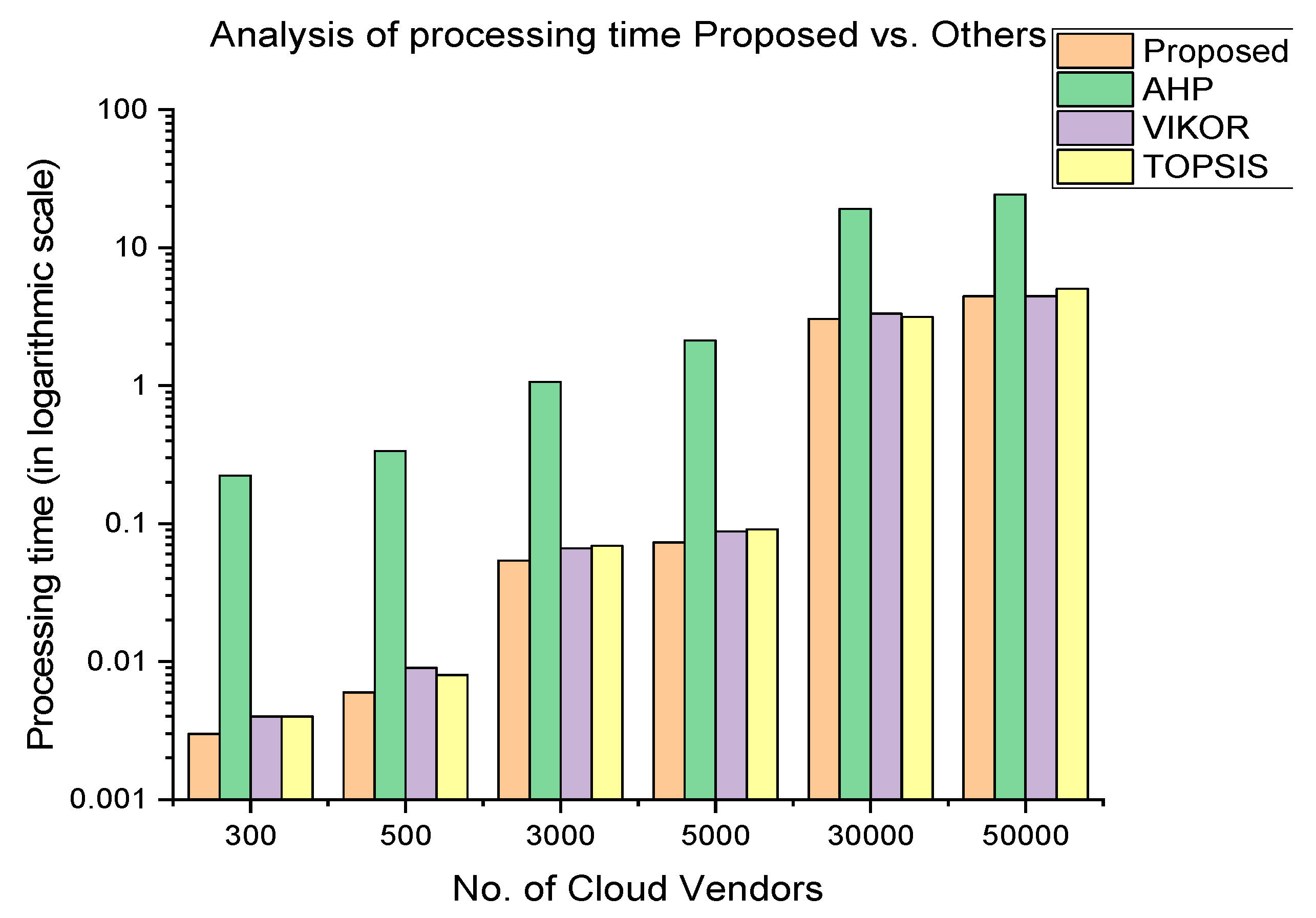
5. Comparative Investigation of Proposed Framework vs. Others

This section deals with the comparative analysis of the proposed framework with other state-of-the-art methods. To ascertain homogeneity in the process of comparison, we consider other methods pertaining to MADM contexts. The methods considered for comparison between the following authors: Garg et al. [1], Kumar et al. [6], Kumar et al. [7], and Liu et al. [12]. The factors for analysis are gathered from the literature and intuition, and used for investigation.

Table 8. Investigation of different factors: Proposed versus others.

Factors	Cloud Vendor Selection Methods
	Proposed	[1]	[6]	[8]	[18]
Data for analysis	PLEs	Crisp			Fuzzy number
Rating style	Likert scale	SLA			Likert scale
Aggregation performed?	yes	no
DMs’ weight considered?	yes	no			yes
Attributes’ weights considered?	yes	no			yes
Prioritization of CVs?	yes
Rank reversal issue	Mitigated from CVs’ perspective	Occurs			Mitigated from CVs’ perspectives
Interrelationship between attributes	Effectively considered	Not considered
Hesitation in preference information	Effectively considered	Not considered			Effectively considered
Partial information on each DM	Effectively considered	Not considered			Not needed

depicts the comparative analysis of different methods.

From Table 8, some of the advantages of the proposed framework can be realized:

• The data structure used for preference information considers both the linguistic evaluation and the occurring probability associated with each term. This allows the rational selection of CV, based on a set of attributes.
• The aggregation of preferences is done effectively by capturing the interrelationship among attributes. This allows effective aggregation of the preferences.
• The hesitation of DMs, during preference elicitation, is also effectively captured during the weight calculation of attributes.
• DMs’ weight values are calculated in a systematic manner by making better use of partial information.
• CVs are prioritized rationally by mitigating rank reversal issue when adequate changes are made to the CVs.

To further realize the strength of the proposed framework, a simulation study is carried out, which determines the processing time of different methods for different CVs being considered. Initially, we formed matrices in a random fashion of order $m\times n$ with PLTS information. Here, $m$ is the number of CVs and $n$ is the number of attributes, and we vary $m$ in a step-wise manner by considering 300, 500, 3000, 5000, 30,000, and 50,000 CVs for analysis. These CVs are rated with respect to six attributes, whose weights are already determined (refer to the previous section). We calculated the processing time of the proposed ranking method and other methods through a PLTS based AHP [43], PLTS based VIKOR [44], and PLTS based TOPSIS [21], presented in Figure 3.

From Figure 3, it is evident that the proposed ranking method consumes less time to execute, compared to other state-of-the-art methods. Also, as the size of $m$ grows, the state-of-the-art methods consume enormous time to execute. Further, the proposed ranking method takes a reasonable amount of time to execute the larger size of $m$. The values presented in Figure 3 are mean values of 100 iterations.

6. Conclusions

This paper proposes a new decision framework under the PLTS context for the rational prioritization of CVs. The framework provides a systematic method for attributes’ weight calculation and DMs’ weight calculation. Also, the preferences from each DM are aggregated effectively by capturing the interrelationship among attributes. CVs are prioritized by extending the COPRAS method under PLTS context and from the sensitivity analysis of weights and strategy values, it can be inferred that the proposed framework is stable.

The proposed framework is a ‘ready-made’ tool for CVs selection. Based on the preference information (PLTS) provided by the DMs, a suitable CV is selected in a systematic manner for the process. The framework helps the vendor plan their strategies on various attributes to compete in the global market and helps customers make rational decisions regarding their purchase and use of services. DMs need some training with the data structure for effectively using the framework to make rational decisions, and these are the implications derived from the study.

For future research, plans have been made to use the concepts proposed in this paper to properly recommend CVs to a group of customers. Also, plans have been made to propose new decision frameworks for CV selection under other fuzzy variants including, picture fuzzy sets [45], m-polar fuzzy sets [46], and neutrosophic fuzzy sets [47].

References

1. Garg, S.K.; Versteeg, S.; Buyya, R. A framework for ranking of cloud computing services. Future Gener. Comput. Syst. 2013, 29, 1012–1023. [Google Scholar] [CrossRef]
2. Buyya, R.; Yeo, C.S.; Venugopal, S.; Broberg, J.; Brandic, I. Cloud computing and emerging IT platforms: Vision, hype, and reality for delivering computing as the 5th utility. Future Gener. Comput. Syst. 2009, 25, 599–616. [Google Scholar] [CrossRef]
3. Garrison, G.; Wakefield, R.L.; Kim, S. The effects of IT capabilities and delivery model on cloud computing success and firm performance for cloud supported processes and operations. Int. J. Inf. Manag. 2015, 35, 377–393. [Google Scholar] [CrossRef]
4. Misra, S.C.; Mondal, A. Identification of a company’s suitability for the adoption of cloud computing and modelling its corresponding Return on Investment. Math. Comput. Model. 2011, 53, 504–521. [Google Scholar]
5. Somu, N.; Kirthivasan, K.; Shankar, S.S. A computational model for ranking cloud service providers using hypergraph based techniques. Future Gener. Comput. Syst. 2017, 68, 14–30. [Google Scholar] [CrossRef]
6. Kumar, R.R.; Mishra, S.; Kumar, C. A Novel Framework for Cloud Service Evaluation and Selection Using Hybrid MCDM Methods. Arab. J. Sci. Eng. 2018, 43, 7015–7030. [Google Scholar] [CrossRef]
7. Kumar, R.R.; Kumar, C. A Multi Criteria Decision Making Method for Cloud Service Selection and Ranking. Int. J. Ambient Comput. Intell. 2018, 9, 1–14. [Google Scholar] [CrossRef]
8. Rădulescu, C.Z.; Rădulescu, D.M.; Harţescu, F. A cloud service providers ranking approach, based on SAW and modified TOPSIS methods. In Proceedings of the 16th International Conference on Informatics in Economy (IE 2017), Bucharest, Romania, 4–5 May 2017. [Google Scholar]
9. Opricovic, S.; Tzeng, G.H. Compromise solution by MCDM methods: A comparative analysis of VIKOR and TOPSIS. Eur. J. Oper. Res. 2004, 156, 445–455. [Google Scholar]
10. Kumar, R.R.; Kumar, C. An evaluation system for cloud service selection using fuzzy AHP. In Proceedings of the 11th International Conference on Industrial and Information Systems (ICIIS 2016), Uttarkhand, India, 3–4 December 2016. [Google Scholar]
11. Patiniotakis, I.; Verginadis, Y.; Mentzas, G. PuLSaR: Preference-based cloud service selection for cloud service brokers. J. Internet Serv. Appl. 2015, 6, 1–14. [Google Scholar] [CrossRef]
12. Liu, S.; Chan, F.T.S.; Ran, W. Decision making for the selection of cloud vendor: An improved approach under group decision-making with integrated weights and objective/subjective attributes. Expert Syst. Appl. 2016, 55, 37–47. [Google Scholar] [CrossRef]
13. Wagle, S.S.; Guzek, M.; Bouvry, P. Cloud service providers ranking based on service delivery and consumer experience. In Proceedings of the 4th IEEE International Conference on Cloud Networking (CloudNet 2015), Niagara Falls, ON, Canada, 5–7 October 2015. [Google Scholar]
14. Krishankumar, R.; Arvinda, S.R.; Amrutha, A.; Premaladha, J.; Ravichandran, K.S. A decision making framework under intuitionistic fuzzy environment for solving cloud vendor selection problem. In Proceedings of the 2017 International Conference on Networks and Advanced Computational Technologies (NetACT), Kerala, India, 20–22 July 2017. [Google Scholar]
15. Krishankumar, R.; Ravichandran, K.S.; Tyagi, S.K. Solving cloud vendor selection problem using intuitionistic fuzzy decision framework. In Neural Computing and Applications; Springer: Berlin, Germany, 2018; pp. 1–14. [Google Scholar]
16. Somu, N.; Gauthama, G.R.; Kirthivasan, K.; Shankar, S.S. A trust centric optimal service ranking approach for cloud service selection. Future Gener. Comput. Syst. 2018, 86, 234–252. [Google Scholar] [CrossRef]
17. Ding, S.; Wang, Z.; Wu, D.; Olson, D.L. Utilizing customer satisfaction in ranking prediction for personalized cloud service selection. Decis. Support Syst. 2017, 93, 1–10. [Google Scholar] [CrossRef]
18. Zheng, X.; Da Xu, L.; Chai, S. Ranking-Based Cloud Service Recommendation. In Proceedings of the 1st International Conference on Edge Computing IEEE 2017, Honolulu, HI, USA, 25–30 June 2017. [Google Scholar]
19. Pan, Y.; Ding, S.; Fan, W.; Li, J.; Yang, S. Trust-enhanced cloud service selection model based on QoS analysis. PLoS ONE 2015, 10, e0143448. [Google Scholar] [CrossRef]
20. Ghosh, N.; Ghosh, S.K.; Das, S.K. SelCSP: A framework to facilitate selection of cloud service providers. IEEE Trans. Cloud Comput. 2015, 3, 66–79. [Google Scholar] [CrossRef]
21. Pang, Q.; Wang, H.; Xu, Z. Probabilistic linguistic term sets in multi-attribute group decision making. Inf. Sci. 2016, 369, 128–143. [Google Scholar] [CrossRef]
22. Rodriguez, R.M.; Martinez, L.; Herrera, F. Hesitant fuzzy linguistic term sets for decision making. IEEE Trans. Fuzzy Syst. 2012, 20, 109–119. [Google Scholar] [CrossRef]
23. Zhang, G.; Dong, Y.; Xu, Y. Consistency and consensus measures for linguistic preference relations based on distribution assessments. Inf. Fusion 2014, 17, 46–55. [Google Scholar] [CrossRef]
24. Zadeh, L.A. The concept of a linguistic variable and its application to approximate reasoning-I. Inf. Sci. 1975, 8, 199–249. [Google Scholar] [CrossRef]
25. Herrera, F.; Herrera-Viedma, E.; Verdegay, J.L. A Sequential Selection Process in Group Decision Making with a Linguistic Assessment Approach. Inf. Sci. 1995, 239, 223–239. [Google Scholar] [CrossRef]
26. Herrera, F.; Herrera-Viedma, E.; Verdegay, J.L. A model of consensus in group decision making under linguistic assessments. Fuzzy Sets Syst. 1996, 78, 73–87. [Google Scholar] [CrossRef]
27. Herrera, F.; Herrera-Viedma, E.; Verdegay, J.L. A rational consensus model in group decision making using linguistic assessments. Fuzzy Sets Syst. 1997, 88, 31–49. [Google Scholar] [CrossRef]
28. Gou, X.; Xu, Z. Novel basic operational laws for linguistic terms, hesitant fuzzy linguistic term sets and probabilistic linguistic term sets. Inf. Sci. 2016, 372, 407–427. [Google Scholar] [CrossRef]
29. Gupta, P.; Mehlawat, M.K.; Grover, N. Intuitionistic fuzzy multi-attribute group decision-making with an application to plant location selection based on a new extended VIKOR method. Inf. Sci. 2016, 370, 184–203. [Google Scholar] [CrossRef]
30. Koksalmis, E.; Kabak, Ö. Deriving Decision Makers’ Weights in Group Decision Making: An Overview of Objective Methods. Inf. Fusion 2018, 49, 146–160. [Google Scholar] [CrossRef]
31. Zavadskas, E.K.; Kaklauskas, A.; Turskis, Z.; Tamošaitiene, J. Selection of the effective dwelling house walls by applying attributes values determined at intervals. J. Civ. Eng. Manag. 2008, 14, 85–93. [Google Scholar] [CrossRef]
32. Zavadskas, E.K.; Turskis, Z.; Kildienė, S. State of art surveys of overviews on MCDM/MADM methods. Technol. Econ. Dev. Econ. 2014, 20, 165–179. [Google Scholar] [CrossRef]
33. Zavadskas, E.K.; Turskis, Z.; Tamošaitiene, J.; Marina, V. Multicriteria selection of project managers by applying grey criteria. Technol. Econ. Dev. Econ. 2008, 14, 462–477. [Google Scholar] [CrossRef]
34. Zavadskas, E.K.; Kaklauskas, A.; Turskis, Z.; Tamošaitien, J. Multi-Attribute Decision-Making Model by Applying Grey Numbers. Inst. Math. Inform. Vilnius. 2009, 20, 305–320. [Google Scholar]
35. Vahdani, B.; Mousavi, S.M.; Tavakkoli-Moghaddam, R.; Ghodratnama, A.; Mohammadi, M. Robot selection by a multiple criteria complex proportional assessment method under an interval-valued fuzzy environment. Int. J. Adv. Manuf. Technol. 2014, 73, 687–697. [Google Scholar] [CrossRef]
36. Gorabe, D.; Pawar, D.; Pawar, N. Selection Of Industrial Robots using Complex Proportional Assessment Method. Am. Int. J. Res. Sci. Technol. Eng. Math. Sci. Technol. Eng. Math. 2014, 5, 140–143. [Google Scholar]
37. Chatterjee, P.; Chakraborty, S. Material selection using preferential ranking methods. Mater. Des. 2012, 35, 384–393. [Google Scholar] [CrossRef]
38. Chatterjee, P.; Athawale, V.M.; Chakraborty, S. Materials selection using complex proportional assessment and evaluation of mixed data methods. Mater. Des. 2011, 32, 851–860. [Google Scholar] [CrossRef]
39. Mousavi-Nasab, S.H.; Sotoudeh-Anvari, A. A comprehensive MCDM-based approach using TOPSIS, COPRAS and DEA as an auxiliary tool for material selection problems. Mater. Des. 2017, 121, 237–253. [Google Scholar] [CrossRef]
40. Chatterjee, K.; Kar, S. A multi-criteria decision making for renewable energy selection using Z-Numbers. Technol. Econ. Dev. Econ. 2018, 24, 739–764. [Google Scholar] [CrossRef]
41. Yazdani, M.; Chatterjee, P.; Zavadskas, E.K.; Hashemkhani Zolfani, S. Integrated QFD-MCDM framework for green supplier selection. J. Clean. Prod. 2017, 142, 3728–3740. [Google Scholar] [CrossRef]
42. Costa, P.M.A.C. Evaluating Cloud Services Using Multicriteria Decision Analysis. Master’s Thesis, Tecnico Lisboa, Lisboa, Portugal, July 2013. [Google Scholar]
43. Xie, W.; Xu, Z.; Ren, Z.; Wang, H. Probabilistic Linguistic Analytic Hierarchy Process and Its Application on the Performance Assessment of Xiongan New Area. Int. J. Inf. Technol. Decis. Mak. 2018, 16, 1–32. [Google Scholar] [CrossRef]
44. Zhang, X.; Xing, X. Probabilistic linguistic VIKOR method to evaluate green supply chain initiatives. Sustainability 2017, 9, 1231. [Google Scholar] [CrossRef]
45. Cường, B.C. Picture fuzzy sets. J. Comput. Sci. Cybern. 2014, 30, 409–420. [Google Scholar] [CrossRef]
46. Chen, J.; Li, S.; Ma, S.; Wang, X. M-Polar fuzzy sets: An extension of bipolar fuzzy sets. Sci. World J. 2014, 2014, 416530. [Google Scholar] [CrossRef] [PubMed]
47. Smarandache, F. Neutrosophic Set—A Generalization of the Intuitionistic Fuzzy Set. J. Def. Resour. Manag. 2010, 1, 107–116. [Google Scholar]
Figure 1. Proposed decision framework for cloud vendor selection.
Symmetry 11 00682 g001
Figure 2. Analysis of strategy values of decision-makers: Equal and unequal weights.
Symmetry 11 00682 g002
Figure 3. Simulation study for analyzing processing time: Proposed versus Others.
Symmetry 11 00682 g003