A Dynamic Multi-Reduction Algorithm for Brain Functional Connection Pathways Analysis

Abstract

Revealing brain functional connection pathways is of great significance in understanding the cognitive mechanism of the brain. In this paper, we present a novel rough set based dynamic multi-reduction algorithm (DMRA) to analyze brain functional connection pathways. First, a binary discernibility matrix is introduced to obtain a reduction, and a reduction equivalence theorem is proposed and proved to verify the feasibility of reduction algorithm. Based on this idea, we propose a dynamic single-reduction algorithm (DSRA) to obtain a seed reduction, in which two dynamical acceleration mechanisms are presented to reduce the size of the binary discernibility matrix dynamically. Then, the dynamic multi-reduction algorithm is proposed, and multi-reductions can be obtained by replacing the non-core attributes in seed reduction. Comparative performance experiments were carried out on the UCI datasets to illustrate the superiority of DMRA in execution time and classification accuracy. A memory cognitive experiment was designed and three brain functional connection pathways were successfully obtained from brain functional Magnetic Resonance Imaging (fMRI) by employing the proposed DMRA. The theoretical and empirical results both illustrate the potentials of DMRA for brain functional connection pathways analysis.

1. Introduction

The brain is an important organ that serves as the center of the nervous system of human [1]. The cerebral cortex plays a key role on brain cognitive functions [2]. A healthy person has corresponding cognitive activities while being stimulated by the external environment. Multiple brain regions in the cerebral cortex cooperate to complete these activities through different brain functional connection pathways [3]. The brain functional connection pathways have an important contribution to understand the brain functional network models [4,5]. Revealing brain functional connection pathways will provide a scientific basis and reference for diagnosis and treatment [6,7].

Analyzing brain functional connection pathways is one of the basic problems in the study of brain function. The component analysis algorithms were common methods in the early stage. Friston et al. proposed a PCA-based brain functional connection pathway analysis method in 1993 [8], and then they studied the function connection between different brain regions when people processed color and emotion tasks in 1999 [9]. Londei et al. used ICA to detect the activated brain areas and analyzed the functional correlation between the relevant areas by the Granger causality test [10]. Although these methods can obtain functional connection model of the whole brain, they wast a lot of time and space. Clustering algorithms are another kind of common methods to divide brain networks and study brain functional pathways, such as center-based algorithms [11] and heuristic algorithms [12]. However, the results of these algorithms depend heavily on the number of clustering centers and other parameters that do not describe the nature of the brain functional pathways itself. In recent years, ROI-based algorithms have become new hotspots to analyze brain functional connection pathways, as the brain data can be effectively simplified [13,14]. The ROIs, namely regions of interests, have to be selected as the prior knowledge empirically [15] while performing brain functional analysis by these methods. The division of brain structure or the coordinates published in the latest research are usually used as the basis for selecting ROIs [16]. Liu et al. obtained a brain functional connection pathway by an attribute reduction algorithm of rough set successfully and interpreted these knowledge from ROIs [17].

The brain functional connection pathways analysis has been widely used to study the neural mechanism associated with different types of mental disorders. They provide a great help in diagnosis, monitoring and treatment of mental disorders. Desseilles et al. found the functional connection pathway is abnormal between frontal parietal lobe network and visual cortex in patients with severe depression [18]. Salomon et al. compared the difference of whole brain function between schizophrenia patients and normal control group in both resting state and working state. The results show that the whole brain functional connection pathways of schizophrenia patients are lower than the normal in both resting state and working state, and the abnormality was more prominent in resting state [19]. Admon et al. compared brain functional connectivity patterns of 33 servicemen in Iraq before and after their service. They found that the subjects with decreased hippocampus gray matter density exhibit more post-traumatic stress disorder (PTSD) symptoms than those with increased hippocampus gray matter density. Meanwhile, the former’s function connection between hippocampus and prefrontal cortex is significantly reduced [20].

However, only a single brain functional connection pathway is obtained by using the previous methods. In fact, there are multi-pathways in the brain, and these multi-pathways are very important for us to understand the relationship between structure and function of different brain regions. The research on multi-pathways will certainly provide more ideas for the study of brain function. Thus, it is necessary to study a multi-reduction method and use it to the analysis of multiple brain functional connection pathways.

A set of multi-reduction contains different attribute combinations, which have the same decision capabilities [21]. Multi-reductions provide more insights from different perspectives than a single reduction and can form a multi-knowledge system [22]. Unfortunately, it is a major challenge to obtain multi-reduction [23]. Wu et al. [24] proposed a method to obtain multi-reduction based on positive region by replacing the non-core attributes. Firstly, the core attributes are collected to get a reduction. Then, the multi-reduction set is obtained through the replacement of non-core attributes one by one. However, their algorithm cost much more time in computing equivalence classes more than once. Thus, it is worth exploring some new reduction approaches to the multi-pathways from functional magnetic resonance imaging analysis.

In this paper, we propose a novel multi-reduction algorithm for analyzing the brain functional connection pathways from functional Magnetic Resonance Imaging (fMRI) data. After proposing and proving a reduction equivalence theorem, a binary discernibility matrix is introduced for obtaining a single reduction dynamically. Since the size of the binary discernibility matrix is dynamically decreased during attribute reduction, the computational time is significantly reduced. Then, the multi-reduction can be obtained by a strategy of non-core attributes replacement. After testing on benchmark data, we employ the proposed algorithm to obtain multiple pathways from brain cognitive functional imaging successfully. The multi-reduction obtained by our algorithm provides a novel comprehensive view for brain functional connection pathways.

2. Multi-Reduction and Binary Discernibility Matrix Methodology

In this section, the relevant concepts of multi-reduction and binary discernibility matrix are defined and the reduction theorems are proved theoretically.

2.1. Multi-Reduction

In rough set theory, an information system [25] is defined as a 4-tuple $S=(U,A,V,f)$, where U is the universe of discourse, a non-empty finite set of N objects $\{x_1,x_2,\cdots ,x_N\}$. A is also a non-empty finite set that contains all attributes. For every $a\in A$, $a:U\to V_a$ and $V_a$ is the value set of the attribute a.

If $A=\{C\cup D\}$, $C\cap D=\varnothing$, the information system is denoted as a decision table by $T=(U,C,D,V,f)$. C and D are, respectively, called the condition attribute and the decision attribute sets. For two subsets of attributes in decision table, the input features form the set C while the class indices are D. Let I be a subset of A, the equivalence relation [26] $IND\left(I\right)$ is denoted as follows.

$$IND\left(I\right)=\left\{\right(x,y)\in U\times U|\forall a\in I,f(x,a)=f(y,a)\}$$

(1)

All equivalence classes of the relation $IND\left(I\right)$ are denoted by $U/IND\left(I\right)$. For simplicity of notation, $U/I$ replaces $U/IND\left(I\right)$. The condition and decision classes are, respectively, noted $U/C$ and $U/D$. For an attributes subset $B\subseteq C$, $U/B=\{B_1,B_2,\cdots ,B_i,\cdots \}$ denotes a partition of the universe, where $B_i$ is an equivalence class of B. The positive region on equivalence classes $U/B$ for D is defined as follows:

$$PO{S}_B\left(D\right)=\bigcup _{X\in U/B\wedge |X/D|=1}X$$

(2)

where $|X/D|$ represents the cardinality of the set $X/D$.

According to the positive region on the equivalence relation of decision attribute D, the reduction can be defined as shown in Definition 1.

Definition 1.

[Reduction] For a given decision table $T=(U,C,D,V,f)$, the attributes subset B is called a reduction of C, if $PO{S}_B\left(D\right)=PO{S}_C\left(D\right)$ and $\forall b\in B$ $PO{S}_B\left(D\right)\ne PO{S}_{(B-\{b\left\}\right)}\left(D\right)$.

According to Definition 1, a reduction is an attributes subset of the condition attributes, which retains the capacity of the same classification to partition the universe as the whole condition attributes. In fact, the reduction is usually unique.

Definition 2.

[Multi-reduction] Let $RED$ represent the multi-reduction set, it is a set including multiple reductions of C defined by Equation (3).

$$RED=\left\{B\right|PO{S}_B\left(D\right)=PO{S}_C\left(D\right),PO{S}_{(B-\{b\left\}\right)}\left(D\right)\ne PO{S}_B\left(D\right)\}.$$

(3)

2.2. Binary Discernibility Matrix

To obtain reduction from an information system, positive region based reduction algorithms [27] have been widely used in the past. However, many symbolic logic operations have to be conducted by using these algorithms. A binary discernibility matrix [28] can transform the equivalence relation between different attributes into a matrix containing only 0 and 1. Thus, the binary discernibility matrix based reduction algorithms are simpler, more intuitive and easier to understand.

Definition 3.

[Binary discernibility matrix] The binary discernibility matrix of the reduced decision table $T=(U,C,D,V,f)$ is denoted by $M=\left(m(x_i,x_j,c_k)\right)$ where $c_k\in C(k=1,2,\cdots ,|C\left|\right)$, $x_i,x_j\in U$. $(x_i,x_j)$ is an unordered object pair and $m(x_i,x_j,c_k)$ can be defined as follows:

$$\begin{array}{c}M=m(x_i,x_j,c_k)=\hfill \\ \left\{\begin{array}{cc}1\hfill & \mathit{if}f(x_i,c_k)\ne f(x_j,c_k),D\left(x_i\right)\ne D\left(x_j\right),x_i,x_j\in U_{pos},\hfill \\ 1\hfill & \mathit{if}f(x_i,c_k)\ne f(x_j,c_k),x_i\in U_{pos},x_j\in U_{neg},\hfill \\ 0\hfill & \mathit{otherwise}.\hfill \end{array}\right.\hfill \end{array}$$

(4)

According to Definition 3, the two objects in positive regions but with different decision values and the two objects in positive and non-positive regions, respectively, are distinguished by “1” in the matrix. Otherwise, the two objects are equivalent, and the corresponding value in the discernibility matrix is “0”.

A reduction equivalence theorem between positive region based reduction algorithms and binary discernibility matrix based algorithms are proposed and proved as follows.

Theorem 1 (Reduction Equivalence Theorem).

For a given decision table $T=(U,C,D,V,f)$, if a reduction is obtained through the binary discernibility matrix, it must be equivalent to a reduction through its positive region.

Proof of Theorem 1.

Let B be a reduction through the binary discernibility matrix M. Let $U_{pos}$ be the objects set of positive region in T. For $\forall {\left[x_i\right]}_B$, $(({\left[x_i\right]}_B\in U_{pos})\wedge \left(\right|{\left[x_i\right]}_B/D|=1))$ according to Equation (4). The objects set of positive region in M is denoted as $U_B^M$. Thus, $U_B^M={\displaystyle \bigcup _{{\left[x_i\right]}_B\in U_{pos}}}{\left[x_i\right]}_B=U_{pos}=PO{S}_B\left(D\right)$. Therefore, $PO{S}_B\left(D\right)=PO{S}_C\left(D\right)$. B is a reduction which satisfies Definition 1, the theorem follows. □

As Theorem 1 illustrated, the binary discernibility matrix provides an efficient approach to obtain the reduction. We just need to partition the objects in different object pairs through the binary discernibility matrix. According to the generated objects pairs by Equation (4), an unordered object pair $(x_i,x_j)$ can be discerned only by considering the attributes $c_k$ with $m(x_i,x_j,c_k)=1$ instead of the whole attributes. All attributes would be added into a candidate reduction set according to the attribute importance that is defined as follows.

$$\zeta \left(c_k\right)=\sum _{i=1}^{n-1}\sum _{j=i+1}^n{m}^{\prime }(x_i,x_j,c_k)$$

(5)

The larger the $\zeta \left(c_k\right)$ is, the more important the $c_k$ is, and the stronger the ability of $c_k$ to partition the object pair $(x_i,x_j)$ is. Especially, $\zeta \left(c_k\right)=0$ means $c_k$ is a redundant attribute and cannot help us to discern any object pair. An attribute is called a core attribute when it can only be used to partition one object pair. The set of core attributes can be collected as follows.

$$I\left(C\right)=\{c_k|\forall x_i,y_i,i\ne j,arg\sum _{k=1}^n{m}^{\prime }(x_i,x_j,c_k)=1\}$$

(6)

If $I\left(C\right)=\varnothing$, any attribute in condition attributes is not a core attribute.

3. Dynamic Multi-Reduction Algorithm

In this section, the dynamic single reduction and multi-reduction algorithm based on a binary discernibility matrix are proposed successively. We analyze these two algorithms in detail.

To obtain multi-reduction, the decision table is transformed into a binary discernibility matrix by using Equation (4). A core attribute set can be obtained by using Equation (6), and then a reduction called a seed reduction is obtained from the core attribute set, as shown in Algorithm 1. In Algorithm 1, two acceleration mechanisms are used in Steps 3 and 4 to dynamically improve the algorithmic efficiency, respectively. Rows and columns that do not affect the next calculation are deleted in Step 3 to reduce the binary discernibility matrix. Then, the attributes with a value of “1” for the first objects pair in the current matrix are chosen in Step 4. Since only these attribute importance have to be calculated by Equation (5), the computational times of the algorithm are greatly reduced. In Steps 5 and 6, attributes are added to the seed reduction one by one according to their importance until the matrix becomes empty.

Algorithm 1 Dynamic Single Reduction Algorithm (DSRA).

Input:      M and the attributes set R, Output:      seed-reduction $R^{\prime }$   1: $M^{\prime }=M$;   2: while$M^{\prime }=\varnothing$do   3:  For $\forall c_k\in R$, the column of attribute $c_k$ and the rows about object pairs which satisfy $(x_i,x_j)\leftarrow argm(x_i,x_j,c_k)=1$ can be deleted to obtain a new reduced matrix $M^{\prime }$;   4:  Choose the object pair $(x_i^{\prime },x_j^{\prime })$ in the first row of new $M^{\prime }$ and calculate the importance of attributes in the set $\widehat{C}=\{c_k|c_k\leftarrow m^{\prime }(x_i^{\prime },x_j^{\prime },c_k^{\prime })=1\}$ by Equation (5);   5:  $c_{max}\leftarrow argmax\left(\zeta \left(c_k\right)\right)$, $c_k\in \widehat{C}$;   6:  $R\leftarrow R\bigcup \left\{c_{max}\right\}$ according the attribute importance one by one;   7: end while   8: if$R\ne C$then   9:  Output the reduction $R^{\prime }=R$;  10: else  11:  There is no reduction.  12: end if

In Algorithm 1, the loop of Steps 2–7 is performed $|C-R|$ times at most. The time complexities of Steps 3–6 are $O\left(\right|R\left|\right)$, $O(|\widehat{C}||U^{\prime }{|}^2)$, $O(|\widehat{C}|)$ and $O\left(\right|C-R\left|\right)$, respectively. Thus, the time complexity of the loop is $max\left(O\right(|C-R\left|\right|R\left|\right),O\left(\right|C-R\left|\right|\widehat{C}||U^{\prime }{|}^2),O(|C-R\left|\right|\widehat{C}{\left|\right),O\left(\right|C-R|}^2\left)\right)$. The time complexity of Algorithm 1 is no more than $O\left(\right|C{|}^2\left|U{|}^2\right)$. $R^{\prime }$, which is obtained based on R, is a seed-reduction for acquiring more reductions used in Algorithm 2.

The different reduction can be obtained by replacing the non-core attributes. According to $R^{\prime }$ outputted by Algorithm 1, any non-core attribute $r^{\prime }$ in $R^{\prime }=I\left(C\right)-R$ can be replaced by attributes in $C-R$. Through recalling Algorithm 1, new reduction can be obtained by the replacement of different $r^{\prime }$. The dynamic multi-reduction algorithm (DMRA) is summarized in Algorithm 2.

In Algorithm 2, after initializing the attributes and multi-reduction set in Step 1, a binary discernibility matrix can be given using Equation (6) in Step 2. Then, the core attribute $I\left(C\right)$ can be obtained using Equation (6) in Step 3. Algorithm 1 is called to find a seed reduction in Step 5, then more reductions are obtained by a non-core attributes replacement strategy from Step 7 to Step 14. Finally, in Steps 15 and 16, we remove the redundancy in the final reduction set $RED$ and output it.

In Algorithm 2, the matrix M according to T is generated in Step 2 and its time complexity is $O\left(\right|U^{\prime }{|}^2)$. The time complexity of Step 3 for getting the core attributes set is $O\left(\right|C\left|\right|U^{\prime }{|}^2)$. The time complexities of calling Algorithm 1 in Steps 5 and 9 is $O\left(\right|C{|}^2\left|U^{\prime }{|}^2\right)$. The loop from Step 7 to Step 14 will run $|R^{\prime }-I\left(C\right)|$ times. The procedure from Step 10 to Step 12 will cost $O\left(\right|R^{\prime }-I\left(C\right)\left|\right)$ time. Thus, the time complexity of Steps 7–14 is ${max\left(O\right(\left|C\right|}^2|U^{\prime }{|}^2|R^{\prime }-I\left(C\right)\left|\right),O\left(\right|R^{\prime }{-I\left(C\right)|}^2\left)\right)$. The time complexity in Step 15 to remove the redundancy reduction is $O(|R^{\prime }-I(C{|}^2)$. Thus, the total time complexity of Algorithm 2 is not more than $O\left(\right|C{|}^3\left|U^{\prime }{|}^2\right)$. It can be found that the amount of the attributes has a greater influence on the time complexity of Algorithm 2.

Algorithm 2 Dynamic Multi-Reduction Algorithm (DMRA).

Input:      Decision table T Output:      Multi-reduction   1: Initialize the attributes set $R=\varnothing$ and multi-reduction set $RED=\varnothing$;   2: Obtain the binary discernibility matrix $M=\left(m(x_i,x_j,c_k)\right)$ by Equation (4);   3: Collect the set of core attribute $I\left(C\right)$ by Equation (6);   4: $R\leftarrow I\left(C\right)$;   5: Obtain a seed reduction $R^{\prime }$ by Algorithm 1;   6: $RED=RED\bigcup \left\{R^{\prime }\right\}$;   7: for$i=\left|I\right(C\left)\right|+1$ to $|R^{\prime }|$ do   8:  $R=R^{\prime }-\left\{r_i\right\},C=C-\left\{r_i\right\},r_i\in R^{\prime }$;   9:  Recall Algorithm 1 to get a new reduction $R_i$;  10:  if $R_i\notin RED$ then  11:   $RED=RED\bigcup \left\{R_i\right\}$;  12:  end if  13:  $R=R^{\prime }+\left\{r_i\right\},C=C+\left\{r_i\right\}$;  14: end for  15: Remove the redundancy in $RED$.  16: Output $RED$.

4. Experimental Results

We carried out multi-reduction experiments on 10 datasets from the UCI Machine Learning Repository to show the superiority of DMRA over PSORA in execution time and classification accuracy. Then, DMRA was used to obtain multiple brain functional connection pathways from brain functional magnetic resonance imaging.

4.1. Test and Comparative Experiments

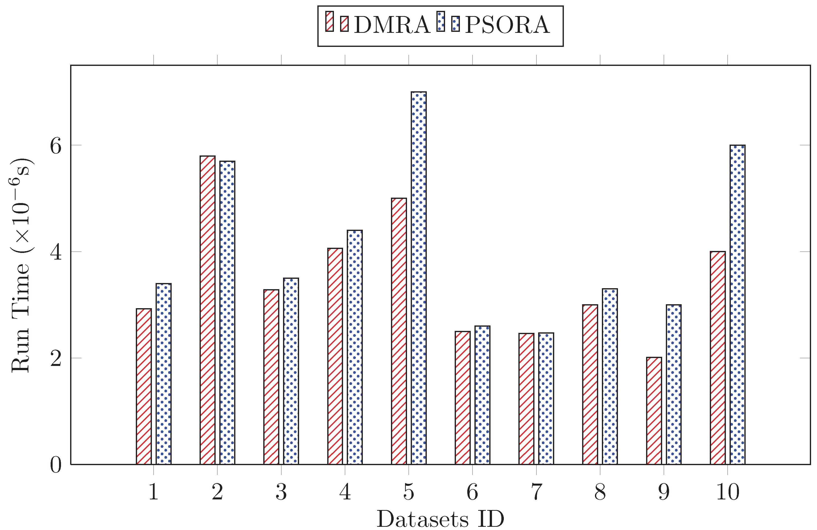
To illustrate the effectiveness of the proposed algorithm, we carried out multi-reduction experiments on 10 well-knowledge benchmark datasets from the UCI Machine Learning Repository, which are listed in

Table 1. Results of DMRA on 10 benchmark datasets.

ID	Data Set	Objects	Condition Attributes	Core Attributes	Reductions
1	Breast Tissue	106	9	1	2
2	Liver Disorders	345	6	0	4
3	Fertility	100	9	1	4
4	Glass	214	9	0	3
5	Heart	270	13	1	4
6	Iris	150	4	0	3
7	Qualitative_Bankruptcy	250	6	0	4
8	Seeds	210	7	0	3
9	SPECT Heart	80	22	2	9
10	Zoo	101	16	2	4

. These datasets such as Glass, Heart and Iris are frequently used to test rough set methods. Some new datasets (e.g., Breast Tissue and SPECT Heart) were also considered in our experiments. The results in the number of core attributes and reductions are also listed in Table 1. Then, we compared the run time of getting the first reduction of DMRA with particle swam optimization based reduction algorithm (PSORA) [17]. The results are shown in Figure 1. We also compared the classification accuracy of DMRA and PSORA (

Table 2. The comparison of classification accuracy.

ID	Datasets	Raw	PSORA	DMRA
				Highest	Lowest	Average
1	Breast Tissue	94.31	95.12	96.21	94.33	95.27
2	Liver Disorders	71.24	71.41	86.33	73.47	80.87
3	Fertility	86.02	87.03	90.45	88.87	89.89
4	Glass	69.23	73.45	80.35	70.34	75.23
5	Heart	82.93	90.23	92.07	90.22	90.45
6	Iris	91.30	93.23	95.23	92.98	94.02
7	Qualitative_Bankruptcy	90.76	92.38	92.58	91.94	92.47
8	Seeds	92.19	94.56	95.81	94.78	95.07
9	SPECT Heart	78.54	82.23	88.13	83.12	85.39
10	Zoo	72.34	77.23	82.04	79.23	81.07

).

As shown in Figure 1, the run time of getting the first reduction by DMRA was always faster than PSORA. The more attributes the dataset contained, the more obvious the speed advantage of the DMRA was. For datasets with fewer attributes, namely Datasets 2, 6 and 7, there was little difference in the running time by using the two algorithms. However, for datasets with more attributes, namely Datasets 5, 9 and 10, DMRA had obvious time advantage. The brain data usually contain many attributes. Thus, the proposed DMRA could obtain reduction results more quickly than PSORA on brain data.

In Table 2, we list the highest, lowest and the average accuracy rate of the different multi-reductions obtained by DMRA, and compare these accuracy rates with raw data and PSORA. No matter using the DMRA or PSORA, the classification accuracy rate was improved, and the best classification accuracy could always be obtained by a reduction obtained by DMRA. The average accuracy rate of multi-reductions obtained by DMRA was higher on all datasets than PSORA. Thus, the proposed DMRA was superior to PSORA in execution time and classification accuracy rate.

Next, we applied the DMRA algorithm to the analysis of multiple brain functional connection pathways.

4.2. Experimental Design

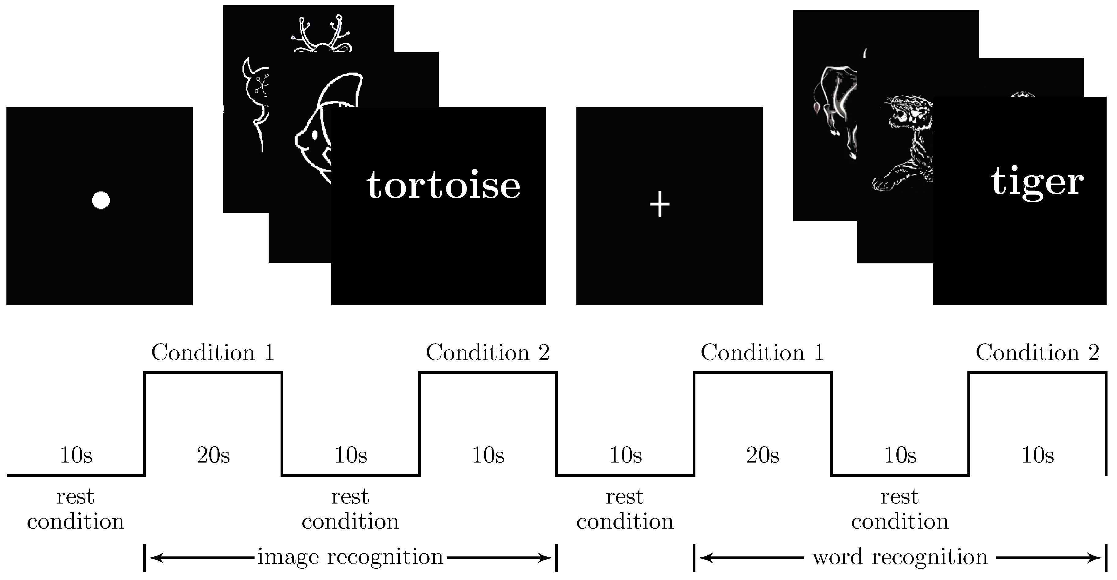
Our brain functional magnetic resonance imaging was acquired using a 3.0T Siemens Magnetron Vision Scanner on 21 young subjects (12 men and 9 women, aged from 17 to 20 years). All subjects were recruited from undergraduate students. Informed consent was obtained before their participation. The cognitive task was a kind of memory experiment, and the cognitive tasks were input in block design [29].

There were two kinds of stimuli in the experiment: images and words. The subjects were demanded to remember the stimuli shown in Condition 1 and to determine whether the stimulus shown in Condition 2 appeared in Condition 1 or not. The block design is shown in Figure 2. Conditions 1 and 2 lasted 12 s and 10 s, respectively, and the rest condition was 10 s so that the subjects could relax.

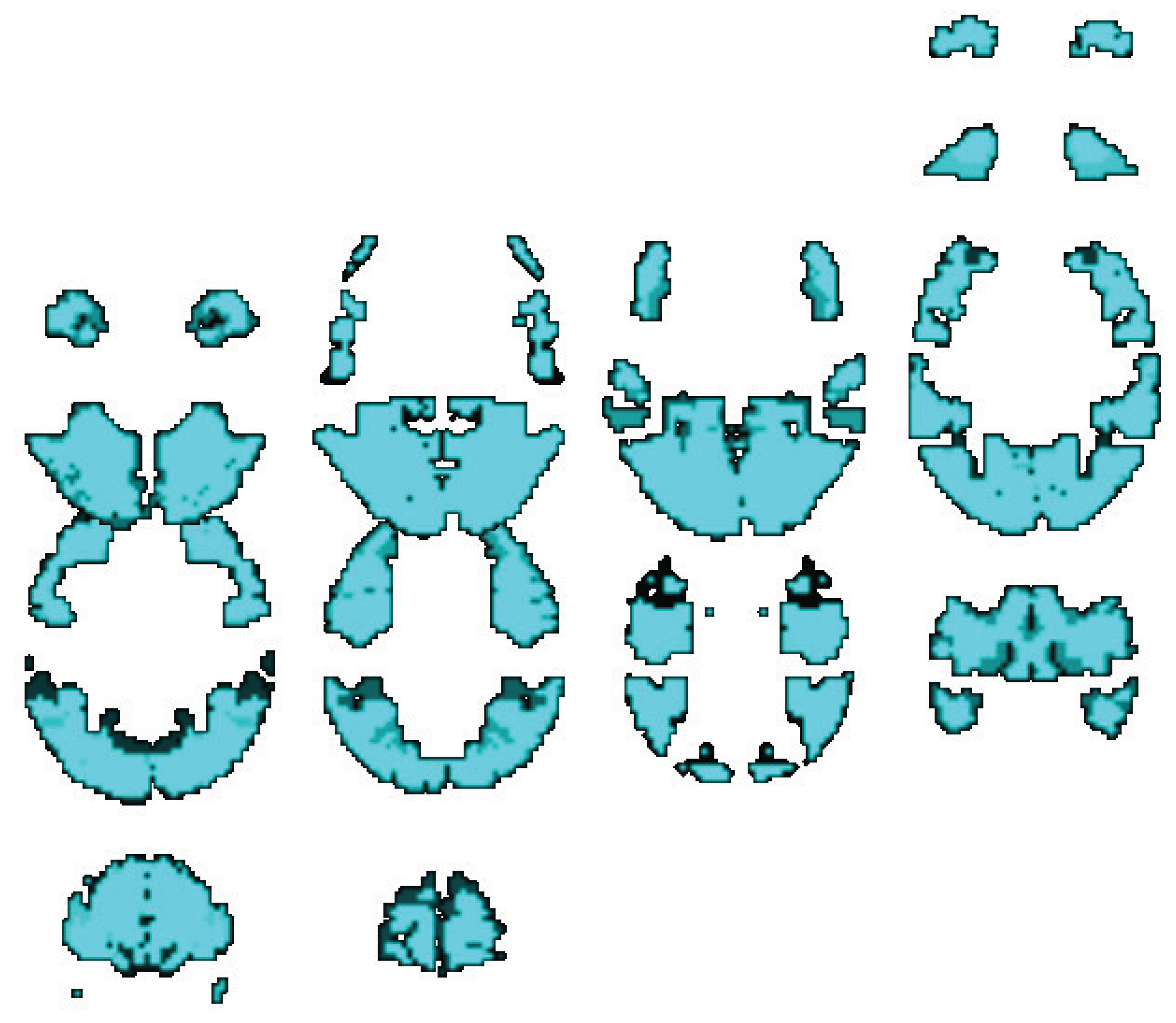
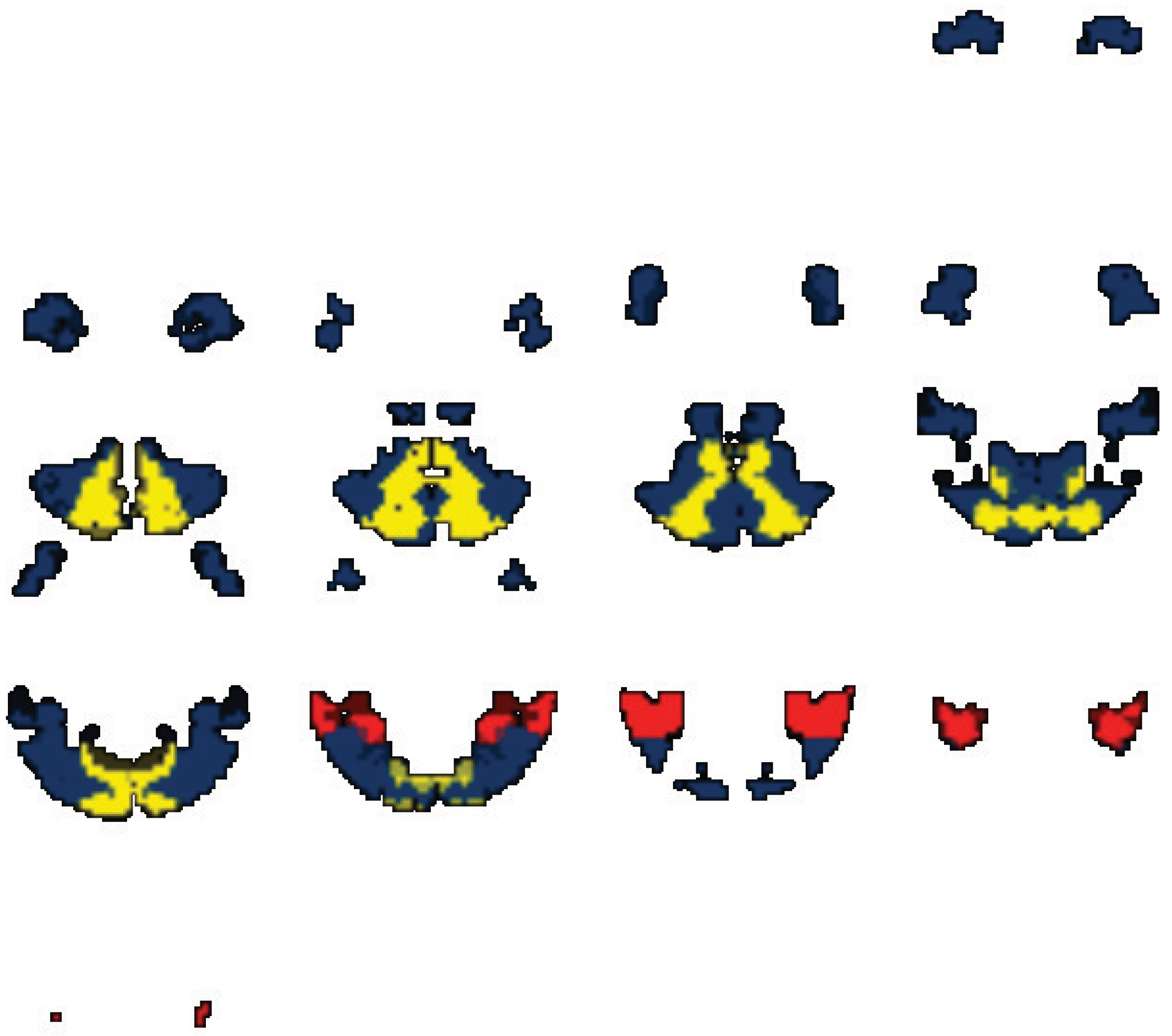
Brodmann Areas (BA) [30] system was used in this study, which was originally defined and numbered by the German anatomist Korbinian Brodmann based on the cytoarchitectural organization of neurons. Each hemisphere of brain is divided into 52 areas in BA. According to our cognitive tasks, we selected 16 areas (BA4, BA6, BA17, BA18, BA19, BA22, BA27, BA37, BA38, BA39, BA40, BA41, BA42, BA44, BA45, and BA46) as the ROIs in the frontal lobe, as shown in Figure 3. For the sake of simplicity in rough set, the brain areas are described with corresponding attribute labels in

Table 3. Description of attribute labels.

Description	Attribute Label	Description	Attribute Label
BA4 area	$c_1$	BA38 area	$c_9$
BA6 area	$c_2$	BA39 area	$c_{10}$
BA17 area	$c_3$	BA40 area	$c_{11}$
BA18 area	$c_4$	BA41 area	$c_{12}$
BA19 area	$c_5$	BA42 area	$c_{13}$
BA22 area	$c_6$	BA44 area	$c_{14}$
BA27 area	$c_7$	BA45 area	$c_{15}$
BA37 area	$c_8$	BA46 area	$c_{16}$

.

We used the statistical parameter mapping (SPM) [31] to obtain the activated brain area from the fMRI images and counted the number of activated voxels in every BA. In SPM, the data preprocessing covered the following steps: time correction, head correction, standardization and Gaussian smooth. Then, the generalized linear model (GLM) was employed to extract the activated voxels. After ascertaining the positions of the activated voxels through Student’s T-test, the number of the activated voxels could be determined within every BA area. Then, the cognitive decision table T could be built, in which the condition attributes were the 16 BAs and the value of each objects in different attributes was the number of activated voxels.

We used the cognitive decision table T as the input of Algorithm 2. The attributes set $R=\varnothing$ and multi-reduction set $RED=\varnothing$ was initialized at first, and the binary discernibility matrix M could be obtained by Equation (4). Then, we obtained the set of core attribute $R=I\left(C\right)=\{BA17,BA19,BA27,BA38,BA39,BA41,BA42,BA45\}$ by Equation (6). Algorithm 1 was used to obtain the first reduction $R^{\prime }=\{BA41,BA40,BA19,BA38,BA17,BA27,BA37,BA39,$$BA45,BA42\}$. Let the set of multi-reductions be $RED=RED\bigcup \left\{R^{\prime }\right\}$. Then, the non-core attributes $\{BA37,BA37\}$ in $R^{\prime }$ were replaced according to Steps 7–14 in Algorithm 2. At the end of the algorithm cycle, $RED$, which contained three reduction results, could be outputted. The $RED$ provided the attribute (namely BA) combinations and their correlations to describe the multiple brain cognitive functional connection pathways.

4.3. Discussion of Experimental Results

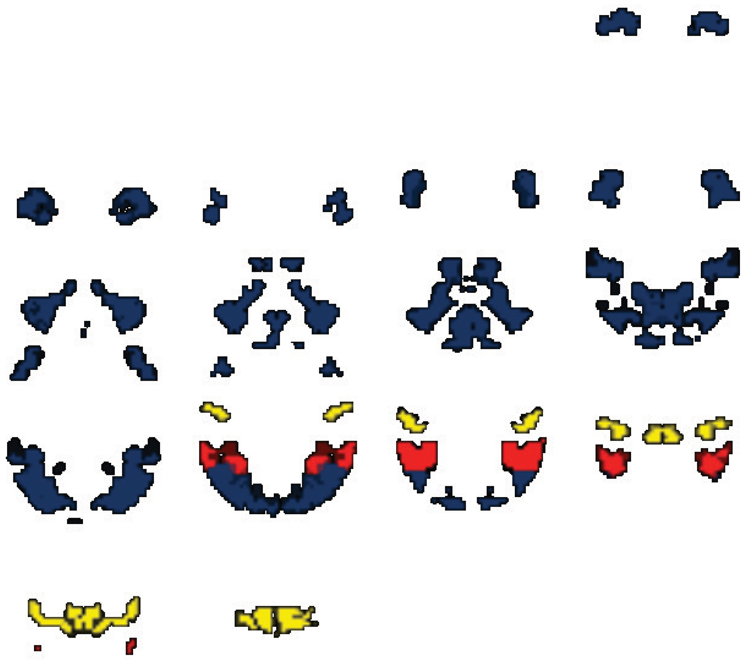
Three reductions in $RED$ were obtained by DMRA algorithm from the cognitive decision table, as shown in

Table 4. Multi-reductions in $RED$.

No.	c1	c2	c3	c4	c5	c6	c7	c8	c9	c10	c11	c12	c13	c14	c15	c16
1	-	-	5	-	3	-	6	7	4	8	2	1	10	-	9	-
2	3	-	5	-	4	-	6	-	7	8	2	1	10	-	9	-
3	3	-	5	-	4	-	6	-	7	8	-	1	10	-	9	2

. The value of the table represents the order of attributes in an attribute reduction and “-” denotes the reduced attributes. The connection pattern of the brain functional pathway was dependent on the order of attributes in a reduction.

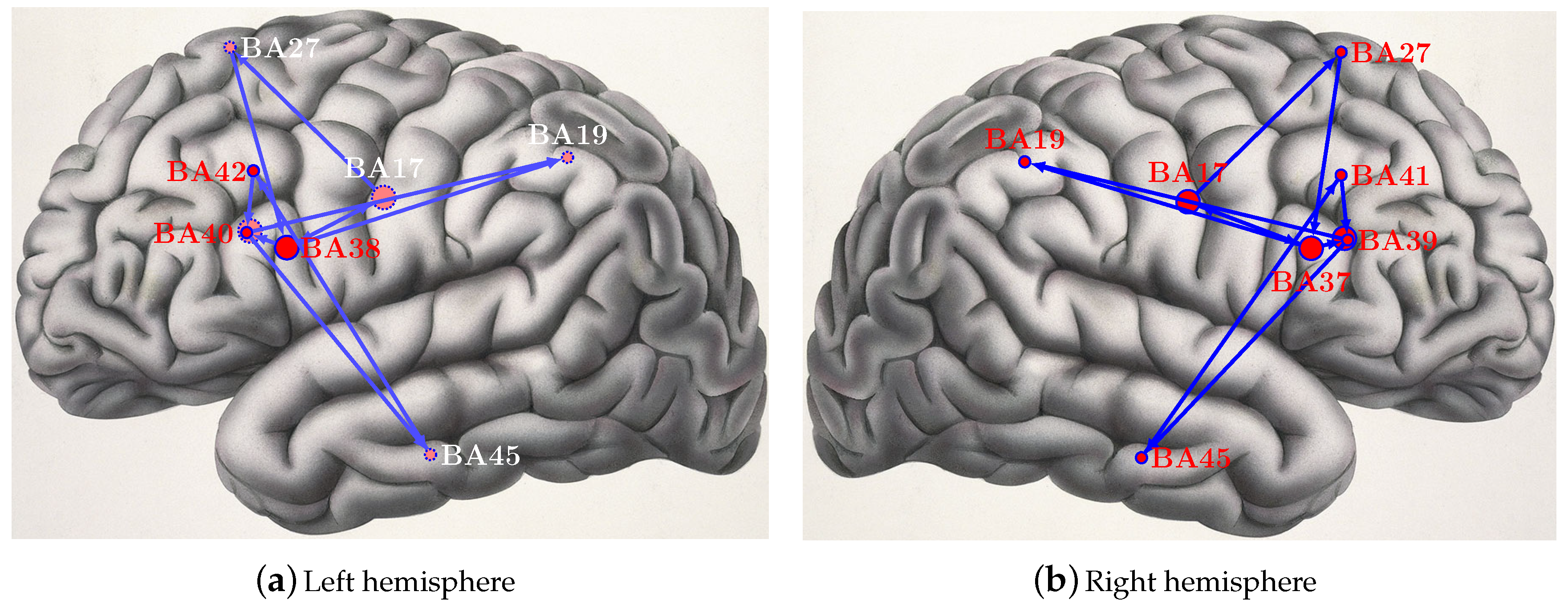
Considering the three reductions obtained through our algorithm (Table 4), BA17, BA19, BA27, BA38, BA39, BA41, BA42 and BA45 were common in these reductions. We regard these eight brain areas as the core attributes, which are closely related to the memory behavior of brain. BA27, BA38, BA41 and BA42 are in the temporal lobe related to memory. BA17 and BA19 are in the occipital lobe related to visual. There are also some areas related to language, including BA39 and BA45. Reductions 1 and 2 have BA40, but BA46 in the frontal cortex replaces BA40 of the same order in Reduction 3. That means BA40 and BA46 may have similar effects in the brain, and they can be replaced by each other sometimes. The coronal position figures of the three reductions for brain functional connection pathways are, respectively, shown in Figure 4, Figure 5 and Figure 6. The common brain areas are the blue highlight in these figures. BA40 or BA46 is the red highlight. The last area in each reduction is the yellow highlight.

According to the three multi-reductions, three brain functional connection pathways about memory can be formed by the order of attributes in Table 4 as follows.

• $\mathrm{BA}41\to \mathrm{BA}40\to \mathrm{BA}19\to \mathrm{BA}38\to \mathrm{BA}17\to \mathrm{BA}27\to \mathrm{BA}37\to \mathrm{BA}39\to \mathrm{BA}45\to \mathrm{BA}42$;
• $\mathrm{BA}41\to \mathrm{BA}40\to \mathrm{BA}4\to \mathrm{BA}19\to \mathrm{BA}17\to \mathrm{BA}27\to \mathrm{BA}38\to \mathrm{BA}39\to \mathrm{BA}45\to \mathrm{BA}42$;
• $\mathrm{BA}41\to \mathrm{BA}46\to \mathrm{BA}4\to \mathrm{BA}19\to \mathrm{BA}17\to \mathrm{BA}27\to \mathrm{BA}38\to \mathrm{BA}39\to \mathrm{BA}45\to \mathrm{BA}42$.

The functional connection pathway derived from the first reduction in Table 4 are shown as an example in Figure 7. The different size of circles represents the activation intensity of brain areas.

5. Conclusions

In this paper, we propose a dynamic multi-reduction approach, in which a binary discernibility matrix is formulated from the decision table in rough set theory. Only the attributes which can discern object pairs are considered, and the attributes importance is measured according to the discernibility matrix. The superiority of DMRA in execution time and classification accuracy are shown by testing on benchmark datasets and comparing with PSORA. Experiments show that the proposed DMRA can effectively deal with attribute reduction of numerical data. It not only helps us to obtain accurate multi-reductions, but also reduces the computational time complexity. The more are attributes contained in the dataset, the more obvious is the advantage of our algorithm over the traditional algorithm. Our DMRA was then applied to analyze brain functional imaging. The areas of interest and its activating features with cognitive tasks was transformed into a decision table. Finally, eight BAs closely related to the memory behavior of brain and three brain functional connection pathways about memory were obtained, while only one brain functional connection pathway can be obtained by the previous approaches. The multi-reduction theory provides a comprehensive analysis approach to complete the knowledge discovery in brain functional imaging. It would make a significant influence on brain functional connection analysis.

References

- Woolsey, T.A.; Hanaway, J.; Gado, M.H. The Brain Atlas: A Visual Guide to the Human Central Nervous System. Neuropathol. Appl. Neurobiol. 2017, 43, 548. [Google Scholar]
- Zelazo, P.D. Executive function: Reflection, iterative reprocessing, complexity, and the developing brain. Dev. Rev. 2015, 38, 55–68. [Google Scholar] [CrossRef]
- Zingg, B.; Chou, X.L.; Zhang, Z.G.; Mesik, L.; Liang, F.; Tao, H.W.; Zhang, L.I. AAV-mediated anterograde transsynaptic tagging: Mapping corticocollicular input-defined neural pathways for defense behaviors. Neuron 2017, 93, 33–47. [Google Scholar] [CrossRef]
- Sporns, O. Contributions and challenges for network models in cognitive neuroscience. Nat. Neurosci. 2014, 17, 652–660. [Google Scholar] [CrossRef] [PubMed]
- Sporns, O.; Betzel, R.F. Modular brain networks. Ann. Rev. Psychol. 2016, 67, 613–640. [Google Scholar] [CrossRef] [PubMed]
- Han, L.; Luo, S.; Yu, J.; Pan, L.; Chen, S. Rule extraction from support vector machines using ensemble learning approach: An application for diagnosis of diabetes. IEEE J. Biomed. Health Inf. 2015, 19, 728–734. [Google Scholar] [CrossRef]
- Solana, J.; Cáceres, C.; García-Molina, A.; Opisso, E.; Roig, T.; Tormos, J.M.; Gómez, E.J. Improving brain injury cognitive rehabilitation by personalized telerehabilitation services: Guttmann Neuropersonal Trainer. IEEE J. Biomed. Health Informat. 2015, 19, 124–131. [Google Scholar] [CrossRef]
- Friston, K.J.; Frith, C.D.; Liddle, P.F.; Frackowiak, R.S. Functional connectivity: The principal-component analysis of large (PET) data sets. J. Cereb. Blood Flow Metab. 1993, 13, 5–14. [Google Scholar] [CrossRef]
- Friston, K.; Phillips, J.; Chawla, D.; Buchel, C. Revealing interactions among brain systems with nonlinear PCA. Hum. Brain Mapp. 1999, 8, 92–97. [Google Scholar] [CrossRef]
- Londei, A.; D’Ausilio, A.; Basso, D.; Sestieri, C.; Del Gratta, C.; Romani, G.; Belardinelli, M.O. Brain network for passive word listening as evaluated with ICA and Granger causality. Brain Res. Bull. 2007, 72, 284–292. [Google Scholar] [CrossRef]
- Ben, D.; Pitskel, N.B.; Pelphrey, K.A. Three systems of insular functional connectivity identified with cluster analysis. Cereb. Cortex 2011, 21, 1498–1506. [Google Scholar]
- Blondel, V.D.; Guillaume, J.L.; Lambiotte, R.; Lefebvre, E. Fast unfolding of communities in large networks. J. Stat. Mech. 2008, 2008, 155–168. [Google Scholar] [CrossRef]
- Hyde, J.S.; Jesmanowicz, A. Cross-correlation: An fMRI signal-processing strategy. Neuroimage 2012, 62, 848–851. [Google Scholar] [CrossRef]
- Fox, M.D.; Greicius, M. Clinical applications of resting state functional connectivity. Front. Syst. Neurosci. 2010, 4, 19. [Google Scholar] [CrossRef] [Green Version]
- Michel, V.; Gramfort, A.; Varoquaux, G.; Eger, E.; Keribin, C.; Thirion, B. A supervised clustering approach for fMRI-based inference of brain states. Pattern Recogn. 2012, 45, 2041–2049. [Google Scholar] [CrossRef] [Green Version]
- Shirer, W.R.; Ryali, S.; Rykhlevskaia, E.; Menon, V.; Greicius, M.D. Decoding subject-driven cognitive states with whole-brain connectivity patterns. Cereb. Cortex 2012, 22, 158–165. [Google Scholar] [CrossRef]
- Liu, H.; Abraham, A.; Zhang, W.; Mcloone, S. A swarm-based rough set approach for fMRI data analysis. Int. J. Innov. Comput. Inf. Control 2011, 7, 3121–3132. [Google Scholar]
- Desseilles, M.; Balteau, E.; Sterpenich, V.; Dang-Vu, T.T.; Darsaud, A.; Vandewalle, G.; Albouy, G.; Salmon, E.; Peters, F.; Schmidt, C. Abnormal neural filtering of irrelevant visual information in depression. J. Neurosci. 2009, 47, S43. [Google Scholar] [Green Version]
- Roy, S.; Maya, B.C.; Avital, H.D.; Ilan, D.; Ronit, W.; Michael, P.; Marina, K.; Moshe, K.; Talma, H.; Rafael, M. Global functional connectivity deficits in schizophrenia depend on behavioral state. J. Neurosci. 2011, 31, 12972. [Google Scholar]
- Admon, R.; Leykin, D.; Lubin, G.; Engert, V.; Andrews, J.; Pruessner, J.; Hendler, T. Stress-induced reduction in hippocampal volume and connectivity with the ventromedial prefrontal cortex are related to maladaptive responses to stressful military service. Hum. Brain Mapp. 2013, 34, 2808–2816. [Google Scholar] [CrossRef]
- Liu, H.; Yang, C.; Zhang, M.; McLoone, S.; Sun, Y. A computational intelligent approach to multi-factor analysis of violent crime information system. Enterp. Inf. Syst. 2014, 1–24. [Google Scholar] [CrossRef]
- Viceconti, M.; Hunter, P.; Hose, R. Big Data, Big Knowledge: Big Data for Personalized Healthcare. IEEE J. Biomed. Health Inf. 2015, 19, 1209–1215. [Google Scholar] [CrossRef]
- Yang, C.; Liu, H.; McLoone, S.; Chen, C.L.P.; Wu, X. A Novel Variable Precision Reduction Approach to Comprehensive Knowledge Systems. IEEE Trans. Cybern. 2018, 48, 661–674. [Google Scholar] [CrossRef] [PubMed]
- Wu, Q.; Bell, D.; Prasad, G.; McGinnity, T.M. A distribution-index-based discretizer for decision-making with symbolic AI approaches. IEEE Trans. Knowl. Data Eng. 2007, 19, 17–28. [Google Scholar] [CrossRef]
- Li, M.; Zhang, X. Information fusion in a multi-source incomplete information system based on information entropy. Entropy 2017, 19, 570. [Google Scholar] [CrossRef]
- Sun, L.; Zhang, X.; Xu, J.; Zhang, S. An attribute reduction method using neighborhood entropy measures in neighborhood rough sets. Entropy 2019, 21, 155. [Google Scholar] [CrossRef]
- Wang, G.; Yu, H.; Li, T. Decision region distribution preservation reduction in decision-theoretic rough set model. Inf. Sci. 2014, 278, 614–640. [Google Scholar]
- Lazo-Cortés, M.S.; Martínez-Trinidad, J.F.; Carrasco-Ochoa, J.A.; Diaz, G.S. A new algorithm for computing reducts based on the binary discernibility matrix. Intell. Data Anal. 2016, 20, 317–337. [Google Scholar] [CrossRef]
- Rozencwajg, P.; Corroyer, D. Strategy development in a block design task. Intelligence 2002, 30, 1–25. [Google Scholar] [CrossRef]
- Saha, S.; Nesterets, Y.; Rana, R.; Tahtali, M.; de Hoog, F.; Gureyev, T. EEG source localization using a sparsity prior based on B rodmann areas. Int. J. Imaging Syst. Technol. 2017, 27, 333–344. [Google Scholar] [CrossRef]
- Booth, B.G.; Keijsers, N.L.; Sijbers, J.; Huysmans, T. STAPP: Spatiotemporal analysis of plantar pressure measurements using statistical parametric mapping. Gait Posture 2018, 63, 268–275. [Google Scholar] [CrossRef] [PubMed]
Figure 1.
The comparison of execution time between DMRA and PSORA.
Figure 2.
Block design of memory cognitive tasks.
Figure 3.
The coronal view of 16 BA areas.
Figure 4.
The coronal position figures of Reduction 1.
Figure 5.
The coronal position figures of Reduction 2.
Figure 6.
The coronal position figures of Reduction 3.