Landslide Susceptibility Mapping for the Muchuan County (China): A Comparison Between Bivariate Statistical Models (WoE, EBF, and IoE) and Their Ensembles with Logistic Regression

Abstract
:1. Introduction
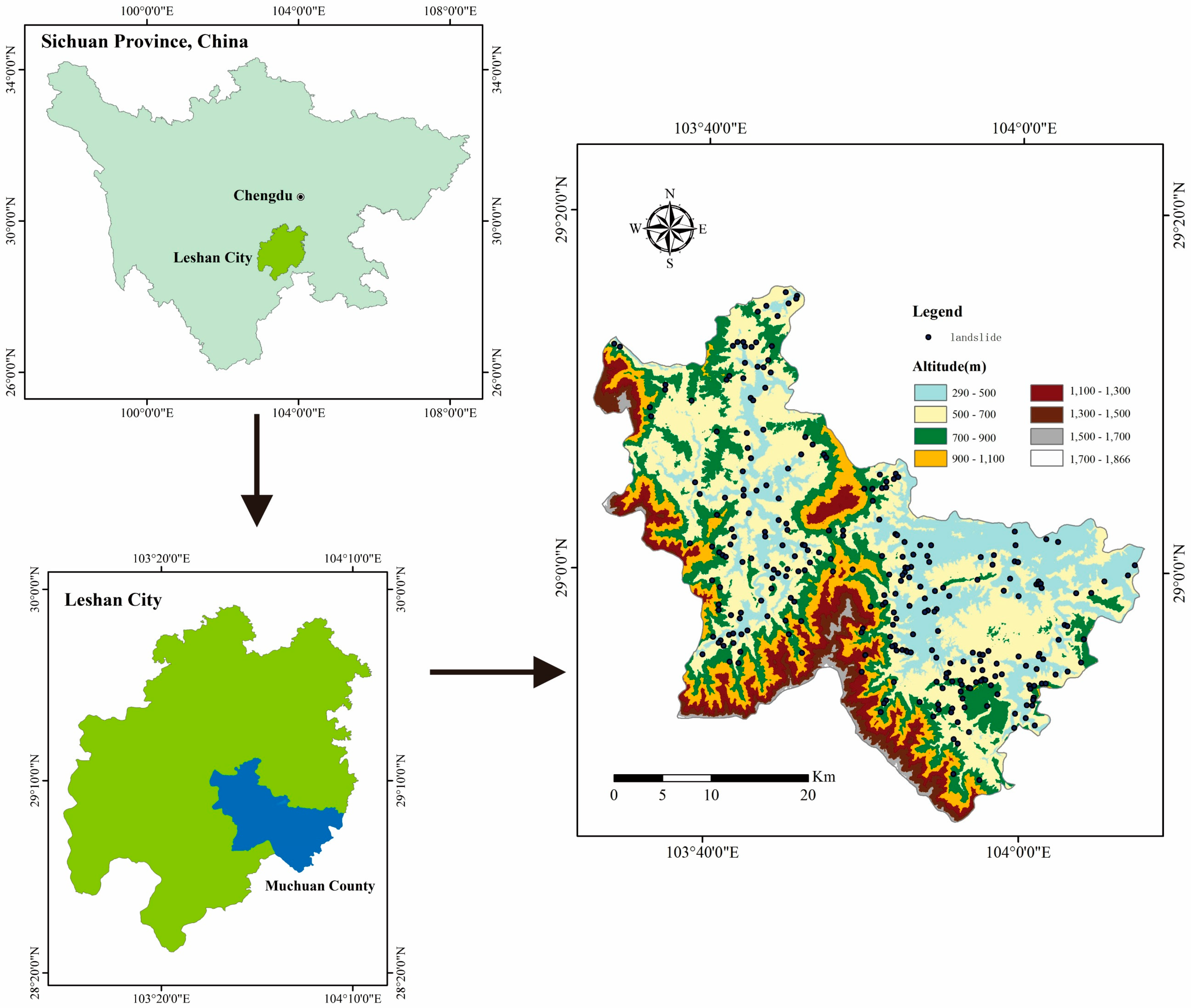
2. Geological and Geomorphological Setting
3. Materials and Methods
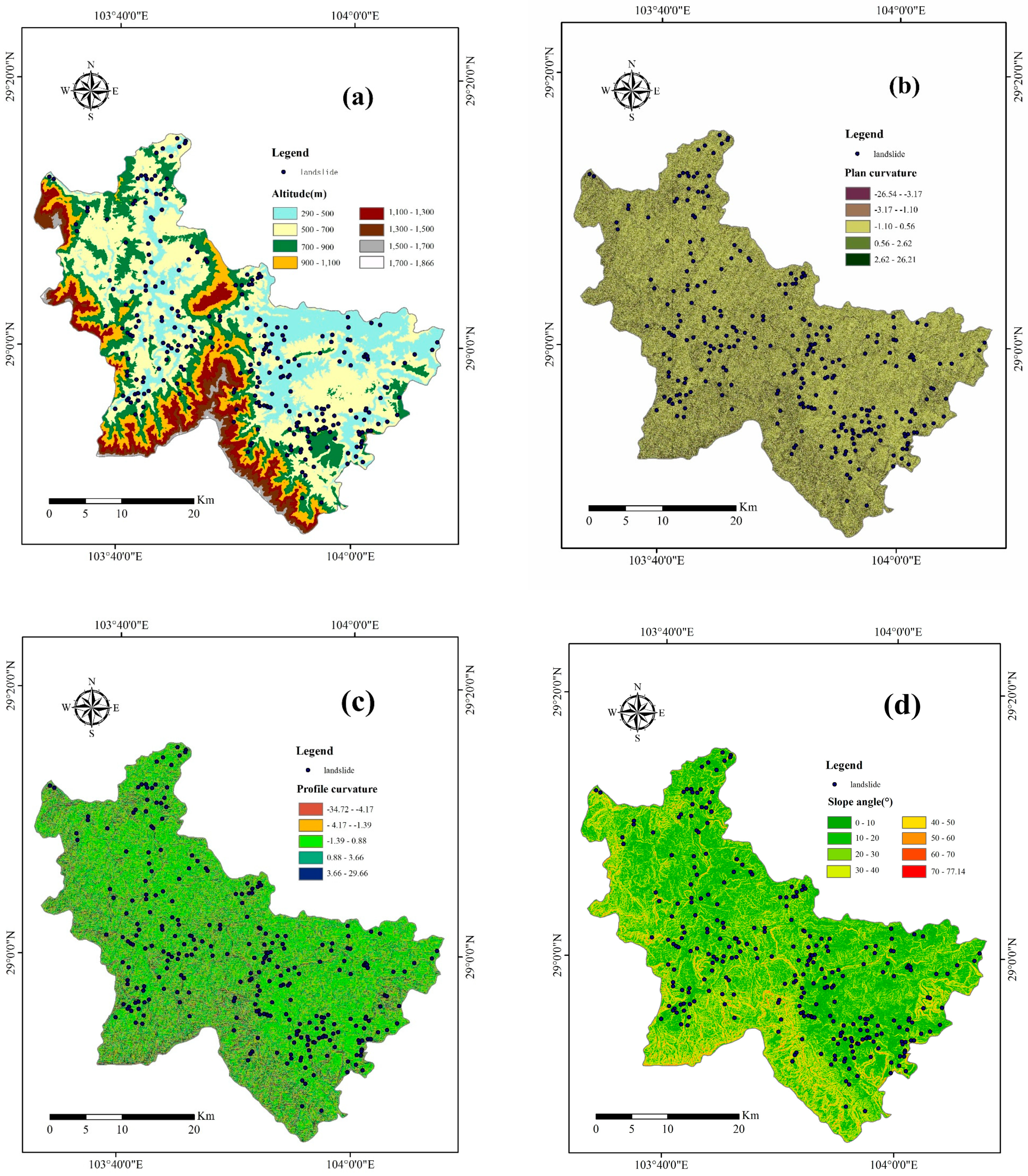
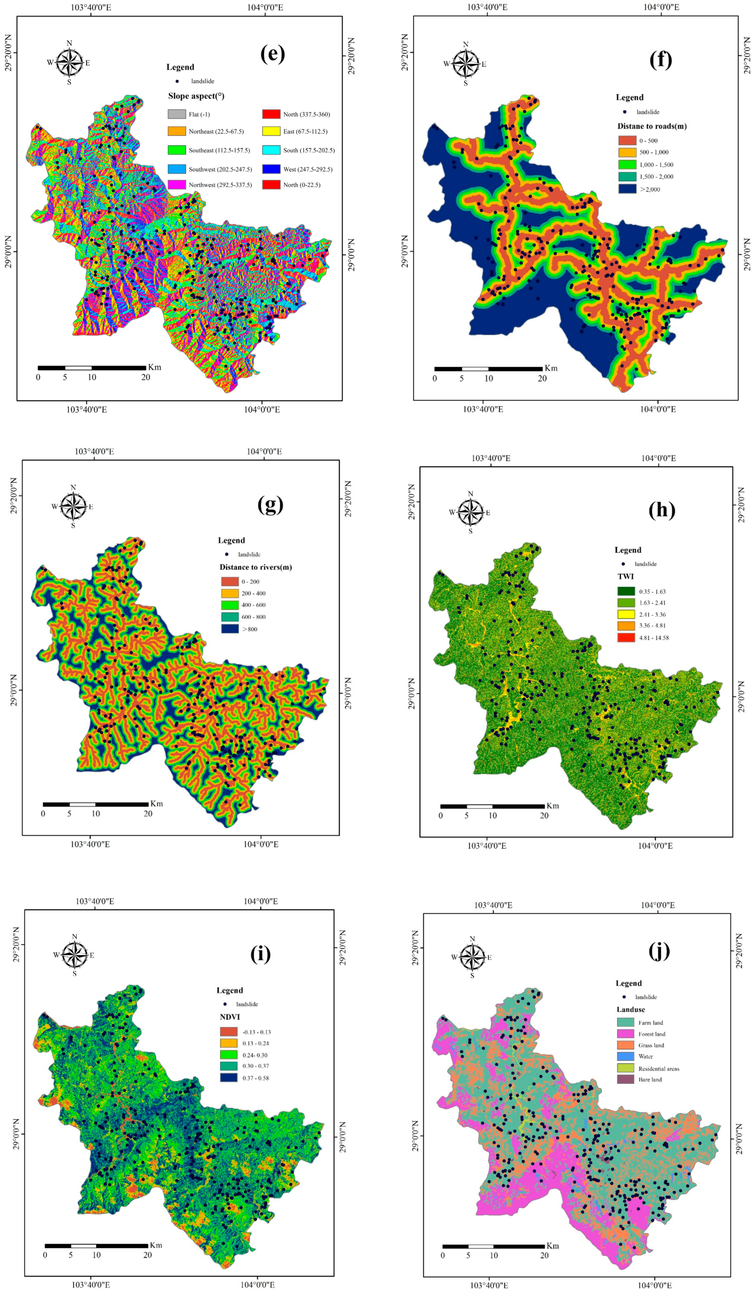
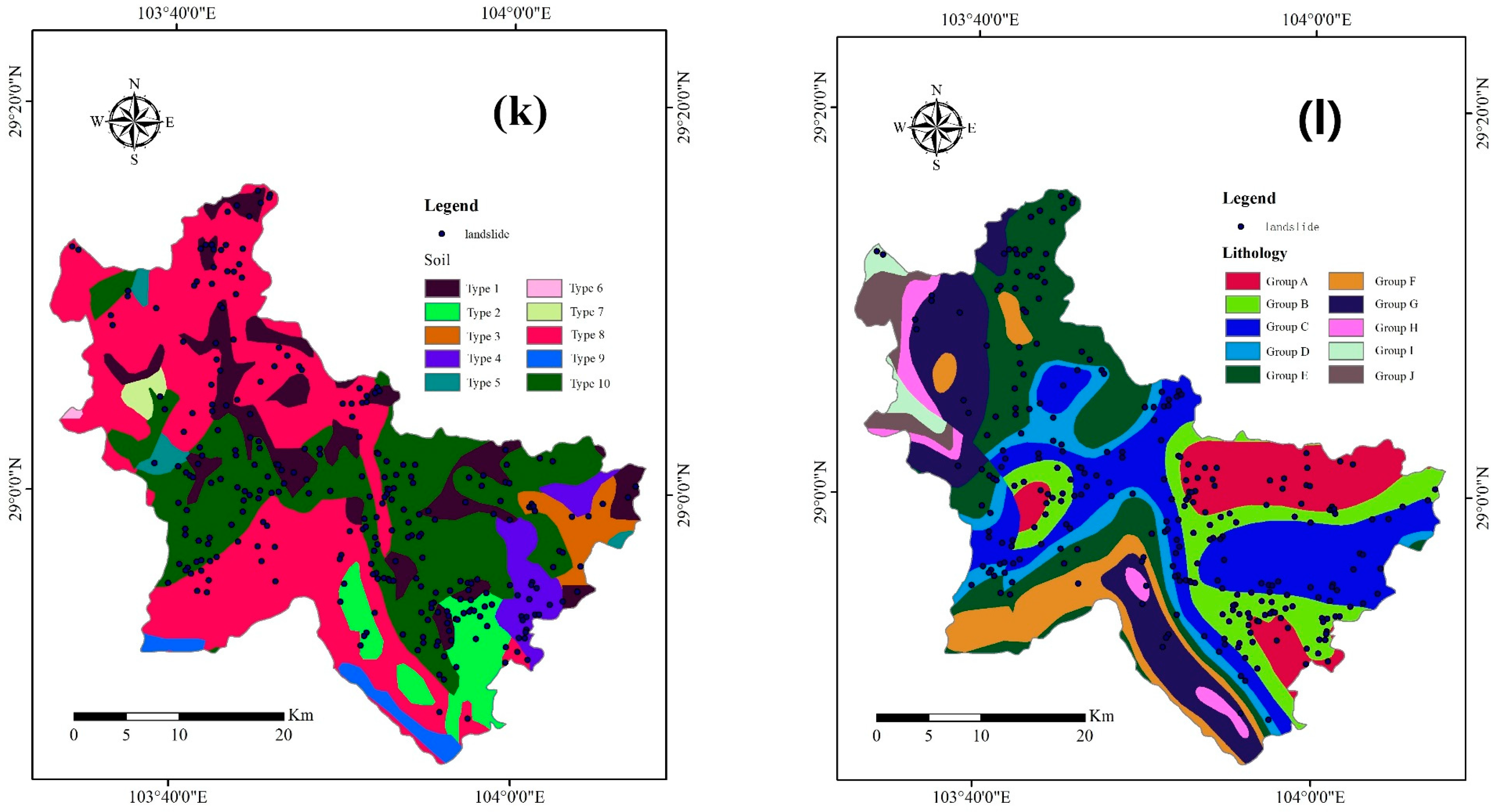
3.1. Landslide Conditioning Factors
3.2. Preparation of Training and Validation Datasets
3.3. Weight of Evidence
3.4. Evidential Belief Function
3.5. Index of Entropy
3.6. Logistic Regression
4. Results and Analysis
4.1. Multicollinearity Analysis
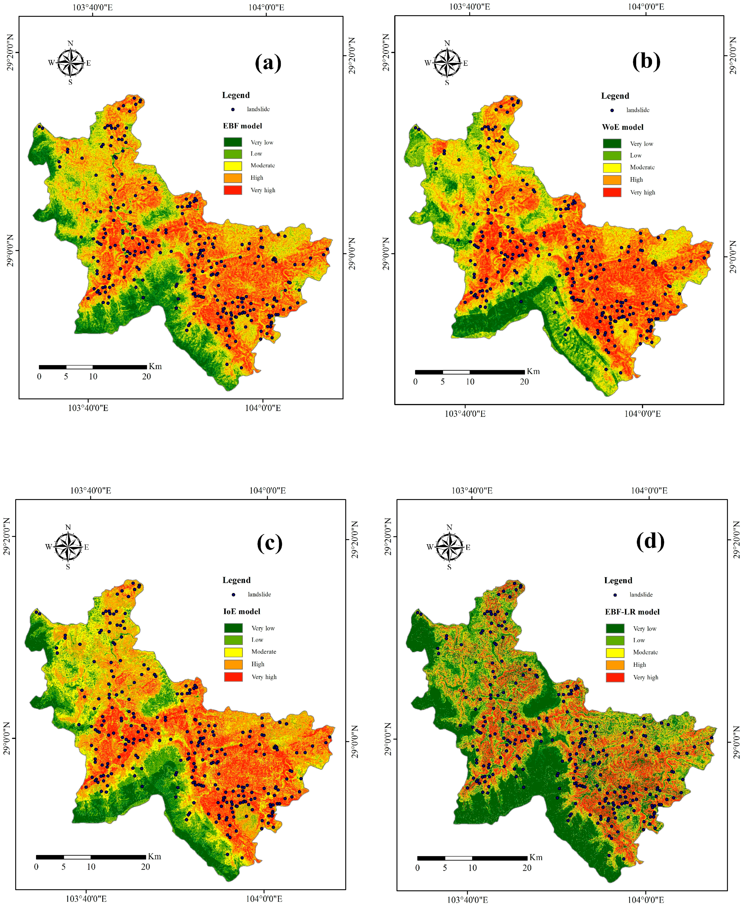
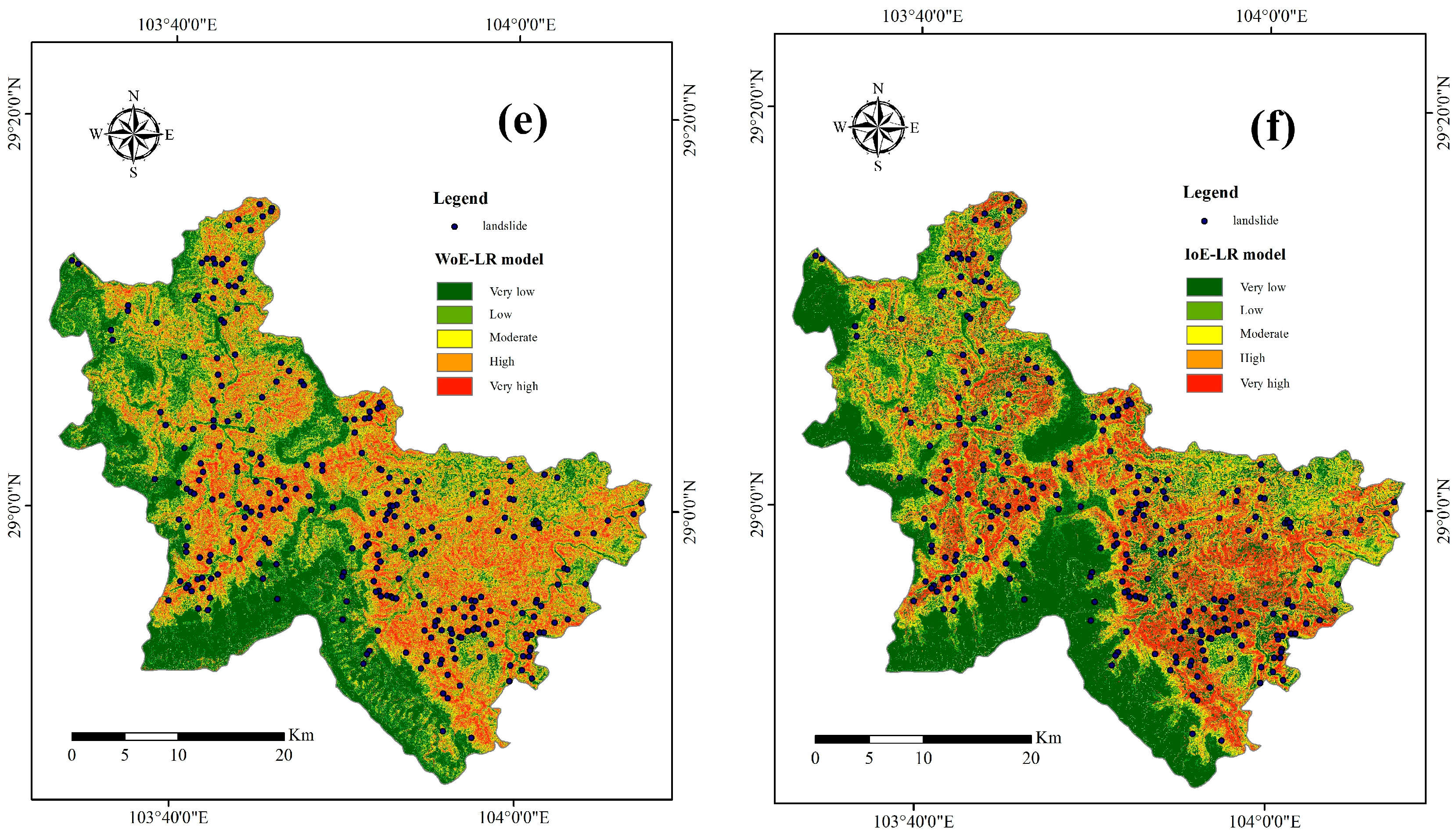
4.2. Generating Landslide Susceptibility Maps
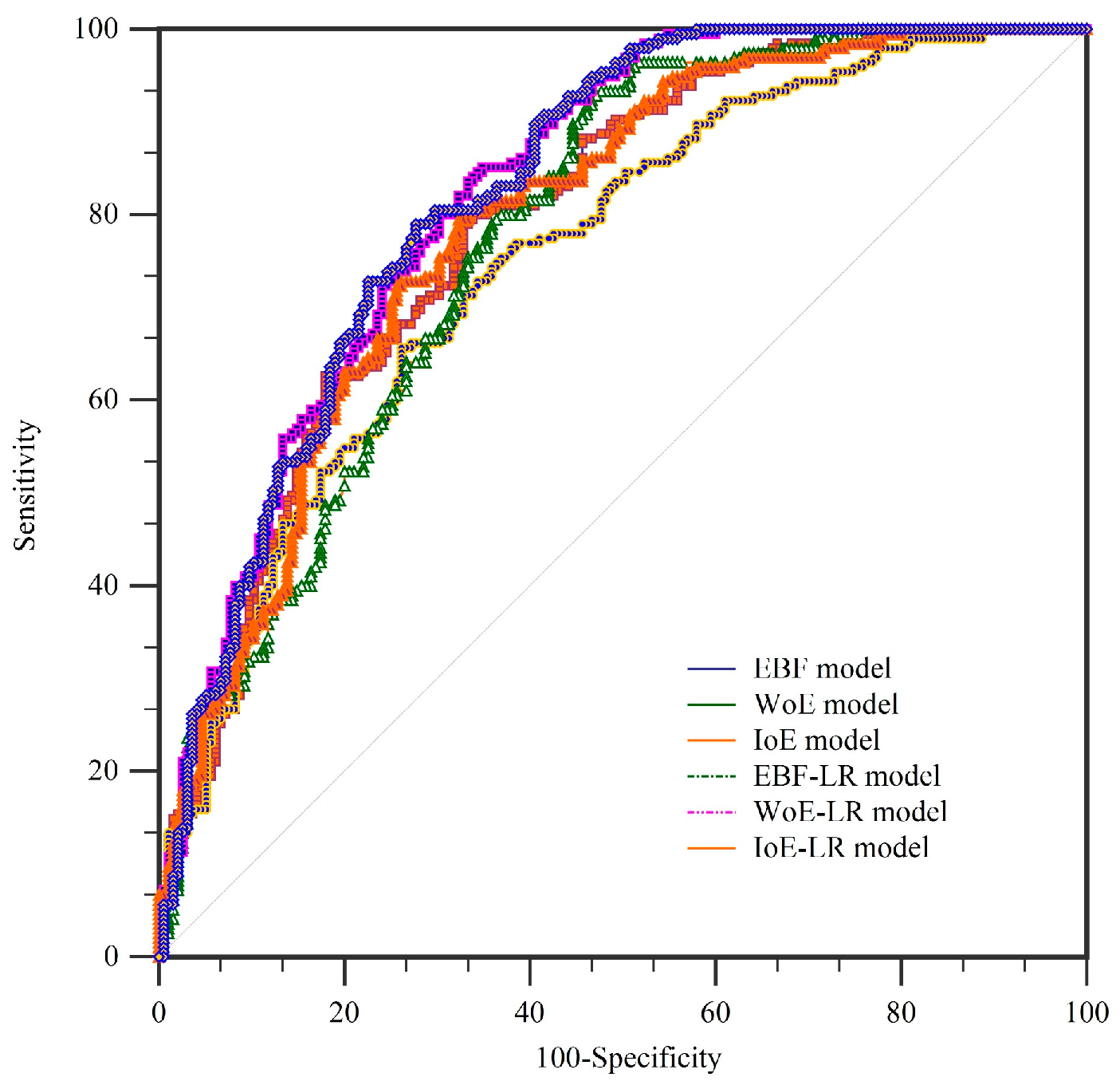
4.3. Model Validation and Comparison
5. Discussions
6. Conclusions
Author Contributions
Acknowledgments
Conflicts of Interest
References
- Grahn, T.; Jaldell, H. Assessment of data availability for the development of landslide fatality curves. Landslides 2017, 14, 1113–1126. [Google Scholar] [CrossRef]
- Huang, F.; Chen, L.; Yin, K.; Huang, J.; Gui, L. Object-oriented change detection and damage assessment using high-resolution remote sensing images, Tangjiao Landslide, Three Gorges Reservoir, China. Environ. Earth Sci. 2018, 77, 183. [Google Scholar] [CrossRef]
- Petrucci, O.; Gullà, G. A simplified method for assessing landslide damage indices. Nat. Hazards 2010, 52, 539–560. [Google Scholar] [CrossRef]
- Hung, L.Q.; Van, N.T.H.; Duc, D.M.; Ha, L.T.C.; Van Son, P.; Khanh, N.H.; Binh, L.T. Landslide susceptibility mapping by combining the analytical hierarchy process and weighted linear combination methods: A case study in the upper Lo River catchment (Vietnam). Landslides 2016, 13, 1285–1301. [Google Scholar] [CrossRef]
- Neuhäuser, B.; Damm, B.; Terhorst, B. GIS-based assessment of landslide susceptibility on the base of the Weights-of-Evidence model. Landslides 2012, 9, 511–528. [Google Scholar] [CrossRef]
- Chen, W.; Li, H.; Hou, E.; Wang, S.; Wang, G.; Panahi, M.; Li, T.; Peng, T.; Guo, C.; Niu, C.; et al. GIS-based groundwater potential analysis using novel ensemble weights-of-evidence with logistic regression and functional tree models. Sci. Total Environ. 2018, 634, 853–867. [Google Scholar] [CrossRef] [PubMed] [Green Version]
- Hong, H.; Pradhan, B.; Xu, C.; Tien Bui, D. Spatial prediction of landslide hazard at the Yihuang area (China) using two-class kernel logistic regression, alternating decision tree and support vector machines. CATENA 2015, 133, 266–281. [Google Scholar] [CrossRef]
- Jebur, M.N.; Pradhan, B.; Tehrany, M.S. Optimization of landslide conditioning factors using very high-resolution airborne laser scanning (LiDAR) data at catchment scale. Remote Sens. Environ. 2014, 152, 150–165. [Google Scholar] [CrossRef]
- Peng, J.; Wang, S.; Wang, Q.; Zhuang, J.; Huang, W.; Zhu, X.; Leng, Y.; Ma, P. Distribution and genetic types of loess landslides in China. J. Asian Earth Sci. 2019, 170, 329–350. [Google Scholar] [CrossRef]
- Broeckx, J.; Vanmaercke, M.; Duchateau, R.; Poesen, J. A data-based landslide susceptibility map of Africa. Earth Sci. Rev. 2018, 185, 102–121. [Google Scholar] [CrossRef]
- Guzzetti, F.; Mondini, A.C.; Cardinali, M.; Fiorucci, F.; Santangelo, M.; Chang, K.-T. Landslide inventory maps: New tools for an old problem. Earth Sci. Rev. 2012, 112, 42–66. [Google Scholar] [CrossRef] [Green Version]
- Li, H.; Xu, Q.; He, Y.; Deng, J. Prediction of landslide displacement with an ensemble-based extreme learning machine and copula models. Landslides 2018, 15, 2047–2059. [Google Scholar] [CrossRef]
- Frattini, P.; Crosta, G.; Carrara, A. Techniques for evaluating the performance of landslide susceptibility models. Eng. Geol. 2010, 111, 62–72. [Google Scholar] [CrossRef]
- Yoshimatsu, H.; Abe, S. A review of landslide hazards in Japan and assessment of their susceptibility using an analytical hierarchic process (AHP) method. Landslides 2006, 3, 149–158. [Google Scholar] [CrossRef]
- Mondal, S.; Maiti, R. Integrating the Analytical Hierarchy Process (AHP) and the frequency ratio (FR) model in landslide susceptibility mapping of Shiv-khola watershed, Darjeeling Himalaya. Int. J. Disaster Risk Sci. 2013, 4, 200–212. [Google Scholar] [CrossRef] [Green Version]
- Myronidis, D.; Papageorgiou, C.; Theophanous, S. Landslide susceptibility mapping based on landslide history and analytic hierarchy process (AHP). Nat. Hazards 2016, 81, 245–263. [Google Scholar] [CrossRef]
- Quan, H.-C.; Lee, B.-G. GIS-based landslide susceptibility mapping using analytic hierarchy process and artificial neural network in Jeju (Korea). KSCE J. Civil Eng. 2012, 16, 1258–1266. [Google Scholar] [CrossRef]
- Wang, Q.; Li, W.; Xing, M.; Wu, Y.; Pei, Y.; Yang, D.; Bai, H. Landslide susceptibility mapping at Gongliu county, China using artificial neural network and weight of evidence models. Geosci. J. 2016, 20, 705–718. [Google Scholar] [CrossRef]
- Zare, M.; Pourghasemi, H.R.; Vafakhah, M.; Pradhan, B. Landslide susceptibility mapping at Vaz Watershed (Iran) using an artificial neural network model: A comparison between multilayer perceptron (MLP) and radial basic function (RBF) algorithms. Arab. J. Geosci. 2013, 6, 2873–2888. [Google Scholar] [CrossRef]
- Feizizadeh, B.; Roodposhti, M.S.; Blaschke, T.; Aryal, J. Comparing GIS-based support vector machine kernel functions for landslide susceptibility mapping. Arab. J. Geosci. 2017, 10, 122. [Google Scholar] [CrossRef]
- Pourghasemi, H.R.; Jirandeh, A.G.; Pradhan, B.; Xu, C.; Gokceoglu, C. Landslide susceptibility mapping using support vector machine and GIS at the Golestan Province, Iran. J. Earth Syst. Sci. 2013, 122, 349–369. [Google Scholar] [CrossRef] [Green Version]
- Wu, X.; Ren, F.; Niu, R. Landslide susceptibility assessment using object mapping units, decision tree, and support vector machine models in the Three Gorges of China. Environ. Earth Sci. 2014, 71, 4725–4738. [Google Scholar] [CrossRef]
- Chen, W.; Zhao, X.; Shahabi, H.; Shirzadi, A.; Khosravi, K.; Chai, H.; Zhang, S.; Zhang, L.; Ma, J.; Chen, Y.; et al. Spatial prediction of landslide susceptibility by combining evidential belief function, logistic regression and logistic model tree. Geocarto Int. 2019. [Google Scholar] [CrossRef]
- Tien Bui, D.; Tuan, T.A.; Klempe, H.; Pradhan, B.; Revhaug, I. Spatial prediction models for shallow landslide hazards: A comparative assessment of the efficacy of support vector machines, artificial neural networks, kernel logistic regression, and logistic model tree. Landslides 2016, 13, 361–378. [Google Scholar] [CrossRef]
- Chen, W.; Shirzadi, A.; Shahabi, H.; Ahmad, B.B.; Zhang, S.; Hong, H.; Zhang, N. A novel hybrid artificial intelligence approach based on the rotation forest ensemble and naïve Bayes tree classifiers for a landslide susceptibility assessment in Langao County, China. Geomat. Nat. Hazards Risk 2017, 8, 1955–1977. [Google Scholar] [CrossRef]
- Hong, H.; Liu, J.; Bui, D.T.; Pradhan, B.; Acharya, T.D.; Pham, B.T.; Zhu, A.X.; Chen, W.; Ahmad, B.B. Landslide susceptibility mapping using J48 Decision Tree with AdaBoost, Bagging and Rotation Forest ensembles in the Guangchang area (China). CATENA 2018, 163, 399–413. [Google Scholar] [CrossRef]
- Pham, B.T.; Tien Bui, D.; Prakash, I. Application of Classification and Regression Trees for Spatial Prediction of Rainfall-Induced Shallow Landslides in the Uttarakhand Area (India) Using GIS. In Climate Change, Extreme Events and Disaster Risk Reduction: Towards Sustainable Development Goals; Mal, S., Singh, R.B., Huggel, C., Eds.; Springer International Publishing: Cham, Switzerland, 2018; pp. 159–170. [Google Scholar]
- Sahana, M.; Sajjad, H. Evaluating effectiveness of frequency ratio, fuzzy logic and logistic regression models in assessing landslide susceptibility: A case from Rudraprayag district, India. J. Mt. Sci. 2017, 14, 2150–2167. [Google Scholar] [CrossRef]
- Aghdam, I.N.; Varzandeh, M.H.M.; Pradhan, B. Landslide susceptibility mapping using an ensemble statistical index (Wi) and adaptive neuro-fuzzy inference system (ANFIS) model at Alborz Mountains (Iran). Environ. Earth Sci. 2016, 75, 553. [Google Scholar] [CrossRef]
- Chen, W.; Panahi, M.; Khosravi, K.; Pourghasemi, H.R.; Rezaie, F.; Parvinnezhad, D. Spatial prediction of groundwater potentiality using ANFIS ensembled with teaching-learning-based and biogeography-based optimization. J. Hydrol. 2019, 572, 435–448. [Google Scholar] [CrossRef]
- Bui, D.T.; Tsangaratos, P.; Ngo, P.-T.T.; Pham, T.D.; Pham, B.T. Flash flood susceptibility modeling using an optimized fuzzy rule based feature selection technique and tree based ensemble methods. Sci. Total Environ. 2019, 668, 1038–1054. [Google Scholar] [CrossRef]
- Chen, W.; Tsangaratos, P.; Ilia, I.; Duan, Z.; Chen, X. Groundwater spring potential mapping using population-based evolutionary algorithms and data mining methods. Sci. Total Environ. 2019, 684, 31–49. [Google Scholar] [CrossRef] [PubMed]
- Rossi, M.; Luciani, S.; Valigi, D.; Kirschbaum, D.; Brunetti, M.T.; Peruccacci, S.; Guzzetti, F. Statistical approaches for the definition of landslide rainfall thresholds and their uncertainty using rain gauge and satellite data. Geomorphology 2017, 285, 16–27. [Google Scholar] [CrossRef]
- Schicker, R.; Moon, V. Comparison of bivariate and multivariate statistical approaches in landslide susceptibility mapping at a regional scale. Geomorphology 2012, 161, 40–57. [Google Scholar] [CrossRef]
- Lee, S.; Pradhan, B. Landslide hazard mapping at Selangor, Malaysia using frequency ratio and logistic regression models. Landslides 2007, 4, 33–41. [Google Scholar] [CrossRef]
- Pradhan, B.; Lee, S. Delineation of landslide hazard areas on Penang Island, Malaysia, by using frequency ratio, logistic regression, and artificial neural network models. Environ. Earth Sci. 2010, 60, 1037–1054. [Google Scholar] [CrossRef]
- Sharma, S.; Mahajan, A.K. A comparative assessment of information value, frequency ratio and analytical hierarchy process models for landslide susceptibility mapping of a Himalayan watershed, India. Bull. Eng. Geol. Environ. 2018. [Google Scholar] [CrossRef]
- Althuwaynee, O.F.; Pradhan, B.; Lee, S. Application of an evidential belief function model in landslide susceptibility mapping. Comput. Geosci. 2012, 44, 120–135. [Google Scholar] [CrossRef]
- Gayen, A.; Saha, S. Application of weights-of-evidence (WoE) and evidential belief function (EBF) models for the delineation of soil erosion vulnerable zones: A study on Pathro river basin, Jharkhand, India. Model. Earth Syst. Environ. 2017, 3, 1123–1139. [Google Scholar] [CrossRef]
- Chen, W.; Shahabi, H.; Shirzadi, A.; Hong, H.; Akgun, A.; Tian, Y.; Liu, J.; Zhu, A.X.; Li, S. Novel hybrid artificial intelligence approach of bivariate statistical-methods-based kernel logistic regression classifier for landslide susceptibility modeling. Bull. Eng. Geol. Environ. 2018. [Google Scholar] [CrossRef]
- Goetz, J.N.; Brenning, A.; Petschko, H.; Leopold, P. Evaluating machine learning and statistical prediction techniques for landslide susceptibility modeling. Comput. Geosci. 2015, 81, 1–11. [Google Scholar] [CrossRef]
- Fan, W.; Wei, X.S.; Cao, Y.B.; Zheng, B. Landslide susceptibility assessment using the certainty factor and analytic hierarchy process. J. Mt. Sci. 2017, 14, 906–925. [Google Scholar] [CrossRef]
- Pradhan, B.; Sameen, M.I. Landslide Susceptibility Modeling: Optimization and Factor Effect Analysis. In Laser Scanning Applications in Landslide Assessment; Pradhan, B., Ed.; Springer International Publishing: Cham, Switzerland, 2017; pp. 115–132. [Google Scholar]
- Mandal, S.P.; Chakrabarty, A.; Maity, P. Comparative evaluation of information value and frequency ratio in landslide susceptibility analysis along national highways of Sikkim Himalaya. Spat. Inf. Res. 2018, 26, 127–141. [Google Scholar] [CrossRef]
- Sarkar, S.; Roy, A.K.; Martha, T.R. Landslide susceptibility assessment using Information Value Method in parts of the Darjeeling Himalayas. J. Geol. Soc. India 2013, 82, 351–362. [Google Scholar] [CrossRef]
- Borrelli, L.; Ciurleo, M.; Gullà, G. Correction to: Shallow landslide susceptibility assessment in granitic rocks using GIS-based statistical methods: The contribution of the weathering grade map. Landslides 2018, 15, 1143–1144. [Google Scholar] [CrossRef]
- Hong, H.; Pourghasemi, H.R.; Pourtaghi, Z.S. Landslide susceptibility assessment in Lianhua County (China): A comparison between a random forest data mining technique and bivariate and multivariate statistical models. Geomorphology 2016, 259, 105–118. [Google Scholar] [CrossRef]
- Mezaal, M.R.; Pradhan, B. An improved algorithm for identifying shallow and deep-seated landslides in dense tropical forest from airborne laser scanning data. CATENA 2018, 167, 147–159. [Google Scholar] [CrossRef]
- Geospatial Data Cloud of Chinese Academy of Sciences (GSCloud). Digital elevation model; Geospatial Data Cloud of Chinese Academy of Sciences: Beijing, China, 2019. [Google Scholar]
- Institute of Soil Science, Chinese Academy of Sciences (ISSCAS). Soil map; Institute of Soil Science, Chinese Academy of Sciences: Nanjing, China, 2019. [Google Scholar]
- National Geological Archives of China (NGAC). Lithology map; National Geological Archives of China: Beijing, China, 2019. [Google Scholar]
- Environmental Systems Research Institude (ESRI). ArcGIS Desktop: Release 10.0; Environmental Systems Research Institude: Redlands, CA, USA, 2010. [Google Scholar]
- Pradhan, B.; Lee, S. Landslide susceptibility assessment and factor effect analysis: Backpropagation artificial neural networks and their comparison with frequency ratio and bivariate logistic regression modelling. Environ. Model. Softw. 2010, 25, 747–759. [Google Scholar] [CrossRef]
- Sheng, T.; Chen, Q. An Altitude Based Landslide and Debris Flow Detection Method for a Single Mountain Remote Sensing Image. In Proceedings of the International Conference on Image and Graphics, Shanghai, China, 13–15 September 2017; Springer: Cham, Switzerland, 2017; pp. 601–610. [Google Scholar]
- Zhou, C.; Yin, K.; Cao, Y.; Ahmed, B.; Li, Y.; Catani, F.; Pourghasemi, H.R. Landslide susceptibility modeling applying machine learning methods: A case study from Longju in the Three Gorges Reservoir area, China. Comput. Geosci. 2018, 112, 23–37. [Google Scholar] [CrossRef] [Green Version]
- Kornejady, A.; Pourghasemi, H.R.; Afzali, S.F. Presentation of RFFR New Ensemble Model for Landslide Susceptibility Assessment in Iran. In Landslides: Theory, Practice and Modelling; Pradhan, S.P., Vishal, V., Singh, T.N., Eds.; Springer International Publishing: Cham, Switzerland, 2019; pp. 123–143. [Google Scholar]
- Samia, J.; Temme, A.; Bregt, A.; Wallinga, J.; Guzzetti, F.; Ardizzone, F.; Rossi, M. Characterization and quantification of path dependency in landslide susceptibility. Geomorphology 2017, 292, 16–24. [Google Scholar] [CrossRef]
- Jacobs, L.; Dewitte, O.; Poesen, J.; Maes, J.; Mertens, K.; Sekajugo, J.; Kervyn, M. Landslide characteristics and spatial distribution in the Rwenzori Mountains, Uganda. J. Afr. Earth Sci. 2017, 134, 917–930. [Google Scholar] [CrossRef]
- Pham, B.T.; Tien Bui, D.; Prakash, I. Bagging based Support Vector Machines for spatial prediction of landslides. Environ. Earth Sci. 2018, 77, 146. [Google Scholar] [CrossRef]
- Zhuang, J.; Peng, J.; Wang, G.; Javed, I.; Wang, Y.; Li, W. Distribution and characteristics of landslide in Loess Plateau: A case study in Shaanxi province. Eng. Geol. 2018, 236, 89–96. [Google Scholar] [CrossRef]
- Chen, W.; Panahi, M.; Tsangaratos, P.; Shahabi, H.; Ilia, I.; Panahi, S.; Li, S.; Jaafari, A.; Ahmad, B.B. Applying population-based evolutionary algorithms and a neuro-fuzzy system for modeling landslide susceptibility. CATENA 2019, 172, 212–231. [Google Scholar] [CrossRef]
- Chen, W.; Pourghasemi, H.R.; Kornejady, A.; Xie, X. GIS-Based Landslide Susceptibility Evaluation Using Certainty Factor and Index of Entropy Ensembled with Alternating Decision Tree Models. In Natural Hazards GIS-Based Spatial Modeling Using Data Mining Techniques; Pourghasemi, H.R., Rossi, M., Eds.; Springer International Publishing: Cham, Switzerland, 2019; pp. 225–251. [Google Scholar]
- Xie, J.; Uchimura, T.; Chen, P.; Liu, J.; Xie, C.; Shen, Q. A relationship between displacement and tilting angle of the slope surface in shallow landslides. Landslides 2019, 16, 1243–1251. [Google Scholar] [CrossRef]
- Braun, A.; Garcia Urquia, E.L.; Moncada Lopez, R.; Yamagishi, H. Landslide Susceptibility Mapping in Tegucigalpa, Honduras, Using Data Mining Methods. In Proceedings of the IAEG/AEG Annual Meeting Proceedings, San Francisco, CA, USA, 17–21 September 2018; Springer International Publishing: Cham, Switzerland, 2019; Volume 1, pp. 207–215. [Google Scholar]
- Can, A.; Dagdelenler, G.; Ercanoglu, M.; Sonmez, H. Landslide susceptibility mapping at Ovacık-Karabük (Turkey) using different artificial neural network models: Comparison of training algorithms. Bull. Eng. Geol. Environ. 2019, 78, 89–102. [Google Scholar] [CrossRef]
- Wang, F.; Xu, P.; Wang, C.; Wang, N.; Jiang, N. Application of a GIS-Based Slope Unit Method for Landslide Susceptibility Mapping along the Longzi River, Southeastern Tibetan Plateau, China. ISPRS Int. J. Geo-Inf. 2017, 6, 172. [Google Scholar] [CrossRef]
- Camilo, D.C.; Lombardo, L.; Mai, P.M.; Dou, J.; Huser, R. Handling high predictor dimensionality in slope-unit-based landslide susceptibility models through LASSO-penalized Generalized Linear Model. Environ. Model. Softw. 2017, 97, 145–156. [Google Scholar] [CrossRef] [Green Version]
- Dou, J.; Yamagishi, H.; Pourghasemi, H.R.; Yunus, A.P.; Song, X.; Xu, Y.; Zhu, Z. An integrated artificial neural network model for the landslide susceptibility assessment of Osado Island, Japan. Nat. Hazards 2015, 78, 1749–1776. [Google Scholar] [CrossRef]
- Arnold, P.; Dorren, L. The Importance of Rockfall and Landslide Risks on Swiss National Roads. In Proceedings of the Engineering Geology for Society and Territory Torino, Basel, Italy, 15–19 September 2014; Springer: Cham, Switzerland, 2015; Volume 6, pp. 671–675. [Google Scholar]
- Dang, V.-H.; Dieu, T.B.; Tran, X.-L.; Hoang, N.-D. Enhancing the accuracy of rainfall-induced landslide prediction along mountain roads with a GIS-based random forest classifier. Bull. Eng. Geol. Environ. 2019, 78, 2835–2849. [Google Scholar] [CrossRef]
- Losasso, L.; Rinaldi, C.; Alberico, D.; Sdao, F. Landslide Risk Analysis Along Strategic Touristic Roads in Basilicata (Southern Italy) Using the Modified RHRS 2.0 Method. In Proceedings of the Computational Science and Its Applications (ICCSA 2017), Trieste, Italy, 3–6 July 2017; Springer: Cham, Switzerland, 2017; pp. 761–776. [Google Scholar]
- Sridhar, B.; Rao, P.J.; Narasimha Rao, G.; Duvvuru, R.; Anusha, C.; Sanyasi Naidu, D.; Srinivas, E.; Sridevi, T.; Madhuri, M.; Padmini, Y. Identification of Landslide Hazard Zones Along the Bheemili Beach Road, Visakhapatnam District, A.P. In Proceedings of International Conference on Remote Sensing for Disaster Management; Springer: Cham, Switzerland, 2019; pp. 515–522. [Google Scholar]
- Cordeira, J.M.; Stock, J.; Dettinger, M.D.; Young, A.M.; Kalansky, J.F.; Ralph, F.M. A 142-year Climatology of Northern California Landslides and Atmospheric Rivers. Bull. Am. Meteorol. Soc. 2019. [Google Scholar] [CrossRef]
- Croissant, T.; Lague, D.; Steer, P.; Davy, P. Rapid post-seismic landslide evacuation boosted by dynamic river width. Nat. Geosci. 2017, 10, 680. [Google Scholar] [CrossRef]
- Göransson, G.; Norrman, J.; Larson, M. Contaminated landslide runout deposits in rivers—Method for estimating long-term ecological risks. Sci. Total Environ. 2018, 642, 553–566. [Google Scholar] [CrossRef] [PubMed]
- Zhao, T.; Dai, F.; Xu, N.-W. Coupled DEM-CFD investigation on the formation of landslide dams in narrow rivers. Landslides 2017, 14, 189–201. [Google Scholar] [CrossRef]
- Canoglu, M.C.; Aksoy, H.; Ercanoglu, M. Integrated approach for determining spatio-temporal variations in the hydrodynamic factors as a contributing parameter in landslide susceptibility assessments. Bull. Eng. Geol. Environ. 2018. [Google Scholar] [CrossRef]
- Chen, W.; Hong, H.; Li, S.; Shahabi, H.; Wang, Y.; Wang, X.; Ahmad, B.B. Flood susceptibility modelling using novel hybrid approach of reduced-error pruning trees with bagging and random subspace ensembles. J. Hydrol. 2019, 575, 864–873. [Google Scholar] [CrossRef]
- Razavizadeh, S.; Solaimani, K.; Massironi, M.; Kavian, A. Mapping landslide susceptibility with frequency ratio, statistical index, and weights of evidence models: A case study in northern Iran. Environ. Earth Sci. 2017, 76, 499. [Google Scholar] [CrossRef]
- Chen, C.-W.; Chen, H.; Oguchi, T. Distributions of landslides, vegetation, and related sediment yields during typhoon events in northwestern Taiwan. Geomorphology 2016, 273, 1–13. [Google Scholar] [CrossRef]
- Fiorucci, F.; Ardizzone, F.; Mondini, A.C.; Viero, A.; Guzzetti, F. Visual interpretation of stereoscopic NDVI satellite images to map rainfall-induced landslides. Landslides 2019, 16, 165–174. [Google Scholar] [CrossRef]
- Sun, W.; Tian, Y.; Mu, X.; Zhai, J.; Gao, P.; Zhao, G. Loess Landslide Inventory Map Based on GF-1 Satellite Imagery. Remote Sens. 2017, 9, 314. [Google Scholar] [CrossRef]
- Bartelletti, C.; Giannecchini, R.; D’Amato Avanzi, G.; Galanti, Y.; Mazzali, A. The influence of geological–morphological and land use settings on shallow landslides in the Pogliaschina T. basin (northern Apennines, Italy). J. Maps 2017, 13, 142–152. [Google Scholar] [CrossRef]
- Diva, I.H.; Irwanto, U.; Nizam, K.; Annur, L.; Sekarjati, D.; Putra, B.G.; Safitri, Y.; Giovandi, E.A.; Nofrizal, A.Y.; Hanif, M.; et al. Investigation Volcanic Land Form and Mapping Landslide Potential at Mount Talang. Sumatra J. Disaster Geogr. Geogr. Educ. 2018, 2, 16–23. [Google Scholar] [CrossRef]
- Persichillo, M.G.; Bordoni, M.; Meisina, C. The role of land use changes in the distribution of shallow landslides. Sci. Total Environ. 2017, 574, 924–937. [Google Scholar] [CrossRef] [PubMed]
- Basher, L.; Betts, H.; Lynn, I.; Marden, M.; McNeill, S.; Page, M.; Rosser, B. A preliminary assessment of the impact of landslide, earthflow, and gully erosion on soil carbon stocks in New Zealand. Geomorphology 2018, 307, 93–106. [Google Scholar] [CrossRef]
- Cheng, C.-H.; Hsiao, S.-C.; Huang, Y.-S.; Hung, C.-Y.; Pai, C.-W.; Chen, C.-P.; Menyailo, O.V. Landslide-induced changes of soil physicochemical properties in Xitou, Central Taiwan. Geoderma 2016, 265, 187–195. [Google Scholar] [CrossRef]
- Rossi, L.M.W.; Rapidel, B.; Roupsard, O.; Villatoro-sánchez, M.; Mao, Z.; Nespoulous, J.; Perez, J.; Prieto, I.; Roumet, C.; Metselaar, K.; et al. Sensitivity of the landslide model LAPSUS_LS to vegetation and soil parameters. Ecol. Eng. 2017, 109, 249–255. [Google Scholar] [CrossRef]
- Thomas, M.A.; Mirus, B.B.; Collins, B.D.; Lu, N.; Godt, J.W. Variability in soil-water retention properties and implications for physics-based simulation of landslide early warning criteria. Landslides 2018, 15, 1265–1277. [Google Scholar] [CrossRef]
- Chen, W.; Sun, Z.; Han, J. Landslide Susceptibility Modeling Using Integrated Ensemble Weights of Evidence with Logistic Regression and Random Forest Models. Appl. Sci. 2019, 9, 171. [Google Scholar] [CrossRef]
- Bièvre, G.; Jongmans, D.; Goutaland, D.; Pathier, E.; Zumbo, V. Geophysical characterization of the lithological control on the kinematic pattern in a large clayey landslide (Avignonet, French Alps). Landslides 2016, 13, 423–436. [Google Scholar] [CrossRef]
- Henriques, C.; Zêzere, J.L.; Marques, F. The role of the lithological setting on the landslide pattern and distribution. Eng. Geol. 2015, 189, 17–31. [Google Scholar] [CrossRef]
- Gu, D.; Huang, D. A complex rock topple-rock slide failure of an anaclinal rock slope in the Wu Gorge, Yangtze River, China. Eng. Geol. 2016, 208, 165–180. [Google Scholar] [CrossRef]
- Watakabe, T.; Matsushi, Y. Lithological controls on hydrological processes that trigger shallow landslides: Observations from granite and hornfels hillslopes in Hiroshima, Japan. CATENA 2019, 180, 55–68. [Google Scholar] [CrossRef]
- Chung, C.-J.F.; Fabbri, A.G. Validation of Spatial Prediction Models for Landslide Hazard Mapping. Nat. Hazards 2003, 30, 451–472. [Google Scholar] [CrossRef]
- Pham, B.T.; Tien Bui, D.; Pourghasemi, H.R.; Indra, P.; Dholakia, M.B. Landslide susceptibility assesssment in the Uttarakhand area (India) using GIS: A comparison study of prediction capability of naïve bayes, multilayer perceptron neural networks, and functional trees methods. Theor. Appl. Climatol. 2017, 128, 255–273. [Google Scholar] [CrossRef]
- Pradhan, B. A comparative study on the predictive ability of the decision tree, support vector machine and neuro-fuzzy models in landslide susceptibility mapping using GIS. Comput. Geosci. 2013, 51, 350–365. [Google Scholar] [CrossRef]
- Pham, B.T. A Novel Classifier Based on Composite Hyper-cubes on Iterated Random Projections for Assessment of Landslide Susceptibility. J. Geol. Soc. India 2018, 91, 355–362. [Google Scholar] [CrossRef]
- Pourghasemi, H.R.; Pradhan, B.; Gokceoglu, C. Application of fuzzy logic and analytical hierarchy process (AHP) to landslide susceptibility mapping at Haraz watershed, Iran. Nat. Hazards 2012, 63, 965–996. [Google Scholar] [CrossRef]
- Tsangaratos, P.; Ilia, I. Comparison of a logistic regression and Naïve Bayes classifier in landslide susceptibility assessments: The influence of models complexity and training dataset size. CATENA 2016, 145, 164–179. [Google Scholar] [CrossRef]
- Ford, A.; Miller, J.M.; Mol, A.G. A Comparative Analysis of Weights of Evidence, Evidential Belief Functions, and Fuzzy Logic for Mineral Potential Mapping Using Incomplete Data at the Scale of Investigation. Nat. Resour. Res. 2016, 25, 19–33. [Google Scholar] [CrossRef]
- Fagin, T.D.; Hoagland, B.W. Patterns from the past: Modeling Public Land Survey witness tree distributions with weights-of-evidence. Plant Ecol. 2011, 212, 207–217. [Google Scholar] [CrossRef]
- Shafizadeh-Moghadam, H.; Tayyebi, A.; Helbich, M. Transition index maps for urban growth simulation: Application of artificial neural networks, weight of evidence and fuzzy multi-criteria evaluation. Environ. Monit. Assess. 2017, 189, 300. [Google Scholar] [CrossRef]
- Wang, Y.; Zhang, M.-S.; Xue, Q.; Wu, S.-D. Risk-based evaluation on geological environment carrying capacity of mountain city—A case study in Suide County, Shaanxi Province, China. J. Mt. Sci. 2018, 15, 2730–2740. [Google Scholar] [CrossRef]
- Deng, M. A Conditional Dependence Adjusted Weights of Evidence Model. Nat. Resour. Res. 2009, 18, 249. [Google Scholar] [CrossRef]
- Weed, D.L. Weight of evidence: A review of concept and methods. Risk Anal. 2005, 25, 1545–1557. [Google Scholar] [CrossRef] [PubMed]
- Cheng, Q. BoostWofE: A New Sequential Weights of Evidence Model Reducing the Effect of Conditional Dependency. Math. Geosci. 2015, 47, 591–621. [Google Scholar] [CrossRef]
- Bronevich, A.G.; Karkishchenko, A.N. The structure of fuzzy measure families induced by upper and lower probabilities. In Statistical Modeling, Analysis and Management of Fuzzy Data; Bertoluzza, C., Gil, M.-Á., Ralescu, D.A., Eds.; Physica-Verlag HD: Heidelberg, Germany, 2002; pp. 160–172. [Google Scholar] [CrossRef]
- Dempster, A.P. Upper and Lower Probabilities Induced by a Multivalued Mapping. In Classic Works of the Dempster-Shafer Theory of Belief Functions; Yager, R.R., Liu, L., Eds.; Springer: Berlin/Heidelberg, Germany, 2008; pp. 57–72. [Google Scholar] [CrossRef]
- Carranza, E.J.M. Data-Driven Evidential Belief Modeling of Mineral Potential Using Few Prospects and Evidence with Missing Values. Nat. Resour. Res. 2015, 24, 291–304. [Google Scholar] [CrossRef]
- Harrison, K.E.; Srivastava, R.P.; Plumlee, R.D. Auditors’ Evaluations of Uncertain Audit Evidence: Belief Functions versus Probabilities. In Belief Functions in Business Decisions; Srivastava, R.P., Mock, T.J., Eds.; Physica-Verlag HD: Heidelberg, Germany, 2002; pp. 161–183. [Google Scholar] [CrossRef]
- Hong, H.; Kornejady, A.; Soltani, A.; Termeh, S.V.R.; Liu, J.; Zhu, A.X.; Ahmad, B.B.; Wang, Y. Landslide susceptibility assessment in the Anfu County, China: Comparing different statistical and probabilistic models considering the new topo-hydrological factor (HAND). Earth Sci. Inform. 2018, 11, 605–622. [Google Scholar] [CrossRef]
- Pradhan, A.M.S.; Kim, Y.-T. Spatial data analysis and application of evidential belief functions to shallow landslide susceptibility mapping at Mt. Umyeon, Seoul, Korea. Bull. Eng. Geol. Environ. 2017, 76, 1263–1279. [Google Scholar] [CrossRef]
- Wang, Q.; Li, W.; Wu, Y.; Pei, Y.; Xing, M.; Yang, D. A comparative study on the landslide susceptibility mapping using evidential belief function and weights of evidence models. J. Earth Syst. Sci. 2016, 125, 645–662. [Google Scholar] [CrossRef] [Green Version]
- Constantin, M.; Bednarik, M.; Jurchescu, M.C.; Vlaicu, M. Landslide susceptibility assessment using the bivariate statistical analysis and the index of entropy in the Sibiciu Basin (Romania). Environ. Earth Sci. 2011, 63, 397–406. [Google Scholar] [CrossRef]
- Singh, V.A.; Pathak, P.; Pandey, P. Monitoring the Teaching—Learning Process via an Entropy Based Index. In Proceedings of Econophysics and Economics of Games, Social Choices and Quantitative Techniques; Springer: Milano, Italy, 2010; pp. 139–146. [Google Scholar]
- Das, A. Logistic Regression. In Encyclopedia of Quality of Life and Well-Being Research; Michalos, A.C., Ed.; Springer: Dordrecht, The Netherland, 2014; pp. 3680–3682. [Google Scholar] [CrossRef]
- Moon, K.-W. Logistic Regression. In Learn ggplot2 Using Shiny App; Moon, K.-W., Ed.; Springer International Publishing: Cham, Switzerland, 2016; pp. 51–54. [Google Scholar] [CrossRef]
- Raja, N.B.; Çiçek, I.; Türkoğlu, N.; Aydin, O.; Kawasaki, A. Correction to: Landslide susceptibility mapping of the Sera River Basin using logistic regression model. Nat. Hazards 2018, 91, 1423. [Google Scholar] [CrossRef]
- Meten, M.; Bhandary, N.P.; Yatabe, R. GIS-based frequency ratio and logistic regression modelling for landslide susceptibility mapping of Debre Sina area in central Ethiopia. J. Mt. Sci. 2015, 12, 1355–1372. [Google Scholar] [CrossRef]
- Weisburd, D.; Britt, C. Logistic Regression. In Statistics in Criminal Justice; Weisburd, D., Britt, C., Eds.; Springer: Boston, MA, USA, 2014; pp. 548–600. [Google Scholar] [CrossRef]
- Pradhan, B. Manifestation of an advanced fuzzy logic model coupled with Geo-information techniques to landslide susceptibility mapping and their comparison with logistic regression modelling. Environ. Ecol. Stat. 2011, 18, 471–493. [Google Scholar] [CrossRef]
- Talaei, R. Landslide susceptibility zonation mapping using logistic regression and its validation in Hashtchin Region, northwest of Iran. J. Geol. Soc. India 2014, 84, 68–86. [Google Scholar] [CrossRef]
- Chen, W.; Pradhan, B.; Li, S.; Shahabi, H.; Rizeei, H.M.; Hou, E.; Wang, S. Novel Hybrid Integration Approach of Bagging-Based Fisher’s Linear Discriminant Function for Groundwater Potential Analysis. Nat. Resour. Res. 2019. [Google Scholar] [CrossRef]
- Bui, D.T.; Ngo, P.-T.T.; Pham, T.D.; Jaafari, A.; Minh, N.Q.; Hoa, P.V.; Samui, P. A novel hybrid approach based on a swarm intelligence optimized extreme learning machine for flash flood susceptibility mapping. CATENA 2019, 179, 184–196. [Google Scholar] [CrossRef]
- Toebe, M.; Cargnelutti Filho, A. Multicollinearity in path analysis of maize (Zea mays L.). J. Cereal Sci. 2013, 57, 453–462. [Google Scholar] [CrossRef]
- International Business Machines Corporation (IBM). SPSS Desktop: Release 22.0; International Business Machines Corporation: Armonk, NY, USA, 2013. [Google Scholar]
- Chen, W.; Shahabi, H.; Zhang, S.; Khosravi, K.; Shirzadi, A.; Chapi, K.; Pham, T.B.; Zhang, T.; Zhang, L.; Chai, H.; et al. Landslide Susceptibility Modeling Based on GIS and Novel Bagging-Based Kernel Logistic Regression. Appl. Sci. 2018, 8, 2540. [Google Scholar] [CrossRef]
- Pourghasemi, H.R.; Rossi, M. Landslide susceptibility modeling in a landslide prone area in Mazandarn Province, north of Iran: A comparison between GLM, GAM, MARS, and M-AHP methods. Theor. Appl. Climatol. 2017, 130, 609–633. [Google Scholar] [CrossRef]
- Pham, B.T.; Tien Bui, D.; Prakash, I.; Dholakia, M.B. Hybrid integration of Multilayer Perceptron Neural Networks and machine learning ensembles for landslide susceptibility assessment at Himalayan area (India) using GIS. CATENA 2017, 149, 52–63. [Google Scholar] [CrossRef]
- Samia, J.; Temme, A.; Bregt, A.; Wallinga, J.; Guzzetti, F.; Ardizzone, F.; Rossi, M. Do landslides follow landslides? Insights in path dependency from a multi-temporal landslide inventory. Landslides 2017, 14, 547–558. [Google Scholar] [CrossRef]
- Xu, D.; Peng, L.; Liu, S.; Wang, X. Influences of Risk Perception and Sense of Place on Landslide Disaster Preparedness in Southwestern China. Int. J. Disaster Risk Sci. 2018, 9, 167–180. [Google Scholar] [CrossRef] [Green Version]
- Devkota, K.C.; Regmi, A.D.; Pourghasemi, H.R.; Yoshida, K.; Pradhan, B.; Ryu, I.C.; Dhital, M.R.; Althuwaynee, O.F. Landslide susceptibility mapping using certainty factor, index of entropy and logistic regression models in GIS and their comparison at Mugling–Narayanghat road section in Nepal Himalaya. Nat. Hazards 2013, 65, 135–165. [Google Scholar] [CrossRef]
- Arabameri, A.; Pradhan, B.; Rezaei, K.; Sohrabi, M.; Kalantari, Z. GIS-based landslide susceptibility mapping using numerical risk factor bivariate model and its ensemble with linear multivariate regression and boosted regression tree algorithms. J. Mt. Sci. 2019, 16, 595–618. [Google Scholar] [CrossRef]
- Chen, W.; Pourghasemi, H.R.; Panahi, M.; Kornejady, A.; Wang, J.; Xie, X.; Cao, S. Spatial prediction of landslide susceptibility using an adaptive neuro-fuzzy inference system combined with frequency ratio, generalized additive model, and support vector machine techniques. Geomorphology 2017, 297, 69–85. [Google Scholar] [CrossRef]
- Jaafari, A.; Najafi, A.; Pourghasemi, H.R.; Rezaeian, J.; Sattarian, A. GIS-based frequency ratio and index of entropy models for landslide susceptibility assessment in the Caspian forest, northern Iran. Int. J. Environ. Sci. Technol. 2014, 11, 909–926. [Google Scholar] [CrossRef] [Green Version]
- Abedini, M.; Tulabi, S. Assessing LNRF, FR, and AHP models in landslide susceptibility mapping index: A comparative study of Nojian watershed in Lorestan province, Iran. Environ. Earth Sci. 2018, 77, 405. [Google Scholar] [CrossRef]
- Demir, G. Landslide susceptibility mapping by using statistical analysis in the North Anatolian Fault Zone (NAFZ) on the northern part of Suşehri Town, Turkey. Nat. Hazards 2018, 92, 133–154. [Google Scholar] [CrossRef]
- Chou, W.-C.; Lin, W.-T.; Lin, C.-Y. Vegetation recovery patterns assessment at landslides caused by catastrophic earthquake: A case study in central Taiwan. Environ. Monit. Assess. 2008, 152, 245. [Google Scholar] [CrossRef]
- Gonzalez-Ollauri, A.; Mickovski, S.B. Hydrological effect of vegetation against rainfall-induced landslides. J. Hydrol. 2017, 549, 374–387. [Google Scholar] [CrossRef] [Green Version]
- Neto, C.; Cardigos, P.; Oliveira, S.C.; Zêzere, J.L. Floristic and vegetation successional processes within landslides in a Mediterranean environment. Sci. Total Environ. 2017, 574, 969–981. [Google Scholar] [CrossRef]


| Group | Lithology | Geologic Ages |
|---|---|---|
| A | Brick red massive allochemical rock, sandstone sandwiched mudstone and siltstone Brick red thin-thick layer silty fine-grained arkose, mudstone Brick red massive allochemical rock, sandstone sandwiched mudstone and siltstone | Cretaceous |
| B | Grayish-purple arkose, siltstone sandwiched mud shale and coquina Bright red mudstone, sandwiched with the same color sandstone and siltstone Grayish-purple arkose, siltstone sandwiched mud shale and coquina | Jurassic |
| C | Yellow-gray feldspar-quartz sandstone interbedded with purple-red mudstone | Jurassic |
| D | Magenta mudstone, quartz sandstone, and siltstone sandwiched biosparite and marl | Jurassic |
| E | Gray sandstone, siltstone, and mudstone Grayish-yellow debris-feldspar, siltstone, mudstone, and coal | Triassic |
| F | Yellow-gray medium-thick dolomite sandwiched limestone, gypsum salt, and salt-soluble breccia | Triassic |
| G | Limestone, dolomite, and shale | Triassic |
| H | Yellow-green siltstone sandwiched with mudstone and coal | Permian |
| I | The upper part is limestone and dolomite and the lower part is shale sandwiched siltstone | Permian |
| J | Grayish-green dense amygdaloidal basalt sandwiched picrite, tuff sand mudstone, shed coal and siliceous rock | Permian |
| Number | Factors | WOE | EBF | IoE | |||
|---|---|---|---|---|---|---|---|
| TOL | VIF | TOL | VIF | TOL | VIF | ||
| 1 | Slope aspect | 0.921 | 1.086 | 0.922 | 1.085 | 0.924 | 1.083 |
| 2 | Altitude | 0.835 | 1.197 | 0.659 | 1.517 | 0.659 | 1.517 |
| 3 | Land use | 0.861 | 1.162 | 0.830 | 1.206 | 0.828 | 1.208 |
| 4 | Lithology | 0.691 | 1.447 | 0.577 | 1.733 | 0.577 | 1.732 |
| 5 | NDVI | 0.980 | 1.020 | 0.953 | 1.050 | 0.954 | 1.048 |
| 6 | Plan curvature | 0.898 | 1.114 | 0.894 | 1.118 | 0.905 | 1.105 |
| 7 | Profile curvature | 0.912 | 1.097 | 0.896 | 1.116 | 0.929 | 1.076 |
| 8 | Distance to rivers | 0.981 | 1.020 | 0.969 | 1.032 | 0.973 | 1.028 |
| 9 | Distance to roads | 0.764 | 1.309 | 0.706 | 1.416 | 0.707 | 1.414 |
| 10 | Slope angle | 0.869 | 1.151 | 0.802 | 1.247 | 0.818 | 1.222 |
| 11 | Soil | 0.798 | 1.253 | 0.717 | 1.394 | 0.723 | 1.384 |
| 12 | TWI | 0.916 | 1.091 | 0.860 | 1.163 | 0.863 | 1.158 |
| Factors | Class | No. of Landslide | No. of Pixels in Domain | W+ | W- | C | Bel | Dis | Unc | Pls | Wj |
|---|---|---|---|---|---|---|---|---|---|---|---|
| Altitude (m) | 290–500 | 42 | 727325 | 0.035 | −0.009 | 0.044 | 0.270 | 0.125 | 0.605 | 0.875 | 0.190 |
| 500–700 | 110 | 1330115 | 0.394 | −0.352 | 0.746 | 0.387 | 0.089 | 0.524 | 0.911 | ||
| 700–900 | 38 | 640772 | 0.061 | −0.014 | 0.076 | 0.277 | 0.125 | 0.598 | 0.875 | ||
| 900–1,100 | 5 | 354758 | −1.375 | 0.081 | −1.456 | 0.066 | 0.137 | 0.797 | 0.863 | ||
| 1,100–1,300 | 0 | 246634 | 0.000 | 0.073 | 0.000 | 0.000 | 0.000 | 1.000 | 1.000 | ||
| 1,300–1,500 | 0 | 144601 | 0.000 | 0.042 | 0.000 | 0.000 | 0.000 | 1.000 | 1.000 | ||
| 1,500–1,700 | 0 | 50150 | 0.000 | 0.014 | 0.000 | 0.000 | 0.000 | 1.000 | 1.000 | ||
| 1,700–1,866 | 0 | 2344 | 0.000 | 0.001 | 0.000 | 0.000 | 0.000 | 1.000 | 1.000 | ||
| Plan curvature | −26.54–−3.17 | 6 | 125417 | −0.153 | 0.005 | −0.159 | 0.165 | 0.199 | 0.636 | 0.801 | 0.009 |
| −3.17–−1.10 | 39 | 592578 | 0.166 | −0.037 | 0.203 | 0.228 | 0.191 | 0.582 | 0.809 | ||
| −1.10–0.56 | 75 | 1660025 | −0.211 | 0.158 | −0.369 | 0.156 | 0.232 | 0.612 | 0.768 | ||
| 0.56–2.62 | 62 | 909888 | 0.200 | −0.081 | 0.282 | 0.236 | 0.182 | 0.582 | 0.818 | ||
| 2.62–26.21 | 13 | 208791 | 0.110 | −0.007 | 0.118 | 0.215 | 0.196 | 0.588 | 0.804 | ||
| Profile curvature | −34.72–−4.17 | 9 | 170680 | −0.056 | 0.003 | −0.059 | 0.199 | 0.201 | 0.600 | 0.799 | 0.004 |
| −4.17–−1.39 | 43 | 777064 | −0.008 | 0.002 | −0.010 | 0.209 | 0.201 | 0.590 | 0.799 | ||
| −1.39–0.88 | 76 | 1299477 | 0.048 | −0.029 | 0.077 | 0.221 | 0.195 | 0.585 | 0.805 | ||
| 0.88–3.66 | 57 | 1012294 | 0.010 | −0.004 | 0.014 | 0.212 | 0.200 | 0.588 | 0.800 | ||
| 3.66–29.66 | 10 | 237184 | −0.280 | 0.018 | −0.297 | 0.159 | 0.204 | 0.637 | 0.796 | ||
| Slope angle (°) | 0–10 | 0 | 738575 | 0.000 | 0.237 | 0.000 | 0.000 | 0.000 | 1.000 | 1.000 | 0.229 |
| 10-20 | 84 | 1233686 | 0.200 | −0.128 | 0.328 | 0.168 | 0.110 | 0.722 | 0.890 | ||
| 20-30 | 63 | 836797 | 0.300 | −0.117 | 0.417 | 0.185 | 0.111 | 0.703 | 0.889 | ||
| 30-40 | 29 | 433617 | 0.182 | −0.029 | 0.210 | 0.165 | 0.122 | 0.714 | 0.878 | ||
| 40-50 | 11 | 186715 | 0.055 | −0.003 | 0.058 | 0.145 | 0.125 | 0.730 | 0.875 | ||
| 50-60 | 8 | 58411 | 0.899 | −0.025 | 0.924 | 0.337 | 0.122 | 0.541 | 0.878 | ||
| 60-70 | 0 | 8690 | 0.000 | 0.002 | 0.000 | 0.000 | 0.000 | 1.000 | 1.000 | ||
| 70–77.14 | 0 | 208 | 0.000 | 0.000 | 0.000 | 0.000 | 0.000 | 1.000 | 1.000 | ||
| Slope aspect | Flat | 0 | 1192 | 0.000 | 0.000 | 0.000 | 0.000 | 0.000 | 1.000 | 1.000 | 0.051 |
| North | 28 | 508458 | −0.013 | 0.002 | −0.015 | 0.124 | 0.111 | 0.764 | 0.889 | ||
| Northeast | 33 | 489376 | 0.190 | −0.035 | 0.225 | 0.152 | 0.107 | 0.741 | 0.893 | ||
| East | 26 | 507513 | −0.085 | 0.014 | −0.099 | 0.115 | 0.113 | 0.772 | 0.887 | ||
| Southeast | 20 | 402282 | −0.115 | 0.014 | −0.129 | 0.112 | 0.113 | 0.775 | 0.887 | ||
| South | 24 | 393289 | 0.090 | −0.012 | 0.102 | 0.138 | 0.110 | 0.753 | 0.890 | ||
| Southwest | 16 | 351360 | −0.203 | 0.020 | −0.223 | 0.103 | 0.113 | 0.784 | 0.887 | ||
| West | 20 | 414052 | −0.144 | 0.018 | −0.162 | 0.109 | 0.113 | 0.778 | 0.887 | ||
| Northwest | 28 | 429177 | 0.157 | −0.024 | 0.181 | 0.147 | 0.108 | 0.744 | 0.892 | ||
| Distance to roads (m) | 0–500 | 69 | 827671 | 0.402 | −0.167 | 0.569 | 0.271 | 0.167 | 0.562 | 0.833 | 0.062 |
| 500–1,000 | 48 | 611007 | 0.343 | −0.091 | 0.433 | 0.255 | 0.180 | 0.564 | 0.820 | ||
| 1,000–1,500 | 36 | 493759 | 0.268 | −0.052 | 0.320 | 0.237 | 0.188 | 0.575 | 0.812 | ||
| 1,500–2,000 | 20 | 366762 | −0.022 | 0.003 | −0.025 | 0.177 | 0.198 | 0.625 | 0.802 | ||
| > 2,000 | 22 | 1197500 | −1.110 | 0.300 | −1.410 | 0.060 | 0.267 | 0.674 | 0.733 | ||
| Distance to rivers (m) | 0–200 | 57 | 1032619 | −0.010 | 0.004 | −0.014 | 0.208 | 0.201 | 0.591 | 0.799 | 0.022 |
| 200–400 | 69 | 844083 | 0.382 | −0.160 | 0.543 | 0.308 | 0.171 | 0.521 | 0.829 | ||
| 400–600 | 29 | 700716 | −0.298 | 0.063 | −0.361 | 0.156 | 0.213 | 0.630 | 0.787 | ||
| 600–800 | 22 | 496233 | −0.229 | 0.033 | −0.263 | 0.167 | 0.207 | 0.626 | 0.793 | ||
| > 800 | 18 | 423048 | −0.271 | 0.032 | −0.303 | 0.160 | 0.207 | 0.633 | 0.793 | ||
| TWI | 0.35–1.63 | 104 | 1318729 | 0.347 | −0.289 | 0.635 | 0.401 | 0.152 | 0.447 | 0.848 | 0.080 |
| 1.63–2.41 | 66 | 1221212 | −0.031 | 0.016 | −0.048 | 0.275 | 0.206 | 0.519 | 0.794 | ||
| 2.41–3.36 | 20 | 653109 | −0.599 | 0.099 | −0.698 | 0.156 | 0.224 | 0.621 | 0.776 | ||
| 3.36–4.81 | 4 | 243618 | −1.223 | 0.051 | −1.274 | 0.083 | 0.213 | 0.703 | 0.787 | ||
| 4.81–14.58 | 1 | 60031 | −1.208 | 0.012 | −1.221 | 0.085 | 0.205 | 0.710 | 0.795 | ||
| NDVI | -0.13–0.13 | 2 | 110968 | −1.130 | 0.022 | −1.151 | 0.077 | 0.206 | 0.717 | 0.794 | 0.037 |
| 0.13–0.24 | 15 | 350282 | −0.264 | 0.026 | −0.290 | 0.184 | 0.206 | 0.610 | 0.794 | ||
| 0.24–0.30 | 41 | 864378 | −0.162 | 0.048 | −0.210 | 0.204 | 0.211 | 0.585 | 0.789 | ||
| 0.30–0.37 | 87 | 1306577 | 0.177 | −0.123 | 0.300 | 0.286 | 0.178 | 0.536 | 0.822 | ||
| 0.37–0.58 | 50 | 864494 | 0.036 | −0.012 | 0.049 | 0.249 | 0.199 | 0.553 | 0.801 | ||
| Land use | Farm land | 140 | 1951094 | 0.252 | −0.449 | 0.701 | 0.421 | 0.108 | 0.471 | 0.892 | 0.207 |
| Forest land | 54 | 1459960 | −0.411 | 0.216 | −0.627 | 0.217 | 0.210 | 0.572 | 0.790 | ||
| Grass land | 0 | 42187 | 0.000 | 0.012 | 0.000 | 0.000 | 0.000 | 1.000 | 1.000 | ||
| Water | 0 | 25016 | 0.000 | 0.007 | 0.000 | 0.000 | 0.000 | 1.000 | 1.000 | ||
| Residential areas | 1 | 16239 | 0.099 | 0.000 | 0.100 | 0.362 | 0.169 | 0.469 | 0.831 | ||
| Bare land | 0 | 2203 | 0.000 | 0.001 | 0.000 | 0.000 | 0.170 | 0.830 | 0.830 | ||
| Soil | Type 1 | 31 | 440582 | 0.232 | −0.038 | 0.271 | 0.188 | 0.096 | 0.716 | 0.904 | 0.194 |
| Type 2 | 12 | 208103 | 0.033 | −0.002 | 0.036 | 0.154 | 0.099 | 0.747 | 0.901 | ||
| Type 3 | 4 | 96481 | −0.296 | 0.007 | −0.304 | 0.111 | 0.100 | 0.789 | 0.900 | ||
| Type 4 | 9 | 147720 | 0.088 | −0.004 | 0.093 | 0.163 | 0.099 | 0.738 | 0.901 | ||
| Type 5 | 1 | 41304 | −0.834 | 0.007 | −0.841 | 0.065 | 0.100 | 0.835 | 0.900 | ||
| Type 6 | 0 | 3783 | 0.000 | 0.001 | 0.000 | 0.000 | 0.000 | 1.000 | 1.000 | ||
| Type 7 | 0 | 27855 | 0.000 | 0.008 | 0.000 | 0.000 | 0.000 | 1.000 | 1.000 | ||
| Type 8 | 54 | 1441599 | −0.398 | 0.207 | −0.605 | 0.100 | 0.123 | 0.777 | 0.877 | ||
| Type 9 | 0 | 68835 | 0.000 | 0.020 | 0.000 | 0.000 | 0.000 | 1.000 | 1.000 | ||
| Type 10 | 84 | 1020437 | 0.389 | −0.218 | 0.608 | 0.220 | 0.080 | 0.700 | 0.920 | ||
| Lithology | A | 26 | 396261 | 0.163 | −0.023 | 0.185 | 0.159 | 0.098 | 0.743 | 0.902 | 0.141 |
| B | 43 | 424981 | 0.596 | −0.120 | 0.715 | 0.245 | 0.089 | 0.666 | 0.911 | ||
| C | 59 | 765703 | 0.323 | −0.113 | 0.437 | 0.186 | 0.089 | 0.724 | 0.911 | ||
| D | 17 | 252004 | 0.190 | −0.016 | 0.207 | 0.163 | 0.099 | 0.738 | 0.901 | ||
| E | 38 | 686719 | −0.008 | 0.002 | −0.010 | 0.134 | 0.100 | 0.766 | 0.900 | ||
| F | 1 | 267436 | −2.702 | 0.074 | −2.777 | 0.009 | 0.108 | 0.883 | 0.892 | ||
| G | 10 | 467170 | −0.958 | 0.091 | −1.048 | 0.052 | 0.110 | 0.839 | 0.890 | ||
| H | 0 | 97599 | 0.000 | 0.028 | 0.000 | 0.000 | 0.000 | 1.000 | 1.000 | ||
| I | 1 | 46018 | −0.942 | 0.008 | −0.951 | 0.053 | 0.101 | 0.846 | 0.899 | ||
| J | 0 | 92808 | 0.000 | 0.027 | 0.000 | 0.000 | 0.000 | 1.000 | 1.000 |
| Landslide Conditioning Factors | WoE-LR | EBF-LR | IoE-LR |
|---|---|---|---|
| Slope aspect | 0.780 | 6.477 | 15.569 |
| Altitude | 1.016 | 8.123 | 11.110 |
| Land use | 0.271 | 1.560 | 2.973 |
| Lithology | 0.484 | 3.951 | 3.567 |
| NDVI | 0.720 | 2.710 | 17.231 |
| Plan curvature | 0.628 | 4.169 | 82.950 |
| Profile curvature | 2.878 | 22.826 | 1239.456 |
| Distance to rivers | 1.045 | 5.298 | 52.206 |
| Distance to roads | 0.467 | 2.634 | 7.665 |
| Slope angle | 3.995 | 20.993 | 12.357 |
| Soil | 0.204 | 2.520 | 2.100 |
| TWI | 0.774 | 3.204 | 11.377 |
| Slope aspect | −1.856 | −17.300 | −17.304 |
| Model | M1 | M2 | M3 | M4 | M5 | M6 | M7 | M8 |
|---|---|---|---|---|---|---|---|---|
| Z | −12.651 | −12.968 | −14.119 | −15.345 | −13.752 | −15.018 | −15.077 | −16.006 |
| Asymp. Sig. (2-tailed) | 0 | 0 | 0 | 0 | 0 | 0 | 0 | 0 |
| Model | M9 | M10 | M11 | M12 | M13 | M14 | M15 | |
| Z | −14.900 | −10.849 | −12.203 | −10.313 | −2.577 | −4.809 | −3.680 | |
| Asymp. Sig. (2-tailed) | 0 | 0 | 0 | 0 | 0 | 0 | 0 |
| Variables | AUC | SE | 95% CI |
|---|---|---|---|
| EBF model | 0.791 | 0.0226 | 0.747 to 0.830 |
| WoE model | 0.753 | 0.0243 | 0.707 to 0.795 |
| IoE model | 0.778 | 0.0233 | 0.734 to 0.819 |
| EBF-LR model | 0.826 | 0.0207 | 0.784 to 0.862 |
| WoE-LR model | 0.792 | 0.0226 | 0.748 to 0.831 |
| IoE-LR model | 0.825 | 0.0208 | 0.784 to 0.861 |
© 2019 by the authors. Licensee MDPI, Basel, Switzerland. This article is an open access article distributed under the terms and conditions of the Creative Commons Attribution (CC BY) license (http://creativecommons.org/licenses/by/4.0/).
Share and Cite
Li, R.; Wang, N. Landslide Susceptibility Mapping for the Muchuan County (China): A Comparison Between Bivariate Statistical Models (WoE, EBF, and IoE) and Their Ensembles with Logistic Regression. Symmetry 2019, 11, 762. https://0-doi-org.brum.beds.ac.uk/10.3390/sym11060762
Li R, Wang N. Landslide Susceptibility Mapping for the Muchuan County (China): A Comparison Between Bivariate Statistical Models (WoE, EBF, and IoE) and Their Ensembles with Logistic Regression. Symmetry. 2019; 11(6):762. https://0-doi-org.brum.beds.ac.uk/10.3390/sym11060762
Chicago/Turabian StyleLi, Renwei, and Nianqin Wang. 2019. "Landslide Susceptibility Mapping for the Muchuan County (China): A Comparison Between Bivariate Statistical Models (WoE, EBF, and IoE) and Their Ensembles with Logistic Regression" Symmetry 11, no. 6: 762. https://0-doi-org.brum.beds.ac.uk/10.3390/sym11060762