Optimizing the Paths of Trains Formed at the Loading Area in a Multi-loop Rail Network


School of Traffic and Transportation, Beijing Jiaotong University, Beijing 100044, China
*
Author to whom correspondence should be addressed.
Symmetry 2019, 11(7), 844; https://0-doi-org.brum.beds.ac.uk/10.3390/sym11070844
Submission received: 29 May 2019
/
Revised: 19 June 2019
/
Accepted: 26 June 2019
/
Published: 1 July 2019
(This article belongs to the Special Issue Multi-Criteria Decision-Making Techniques for Improvement Sustainability Engineering Processes)
Abstract
:Each loop in a multi-loop rail network consists of two segments, both of which have roughly the same conditions and mileage and are approximately symmetrical. This paper is devoted to optimizing the paths of trains formed at the loading area in a multi-loop rail network. To attain this goal, three different situations are analyzed, and two models are proposed for networks with adequate and inadequate capabilities. Computational experiments are also carried out using the commercial software Lingo, with the branch and bound algorithm. The results show that the models can achieve the same solution with different solution times. To solve the problem of path selection for large-scale train flows, a genetic algorithm is also designed and proves to perform well in a set of computational experiments.
1. Introduction
In traditional railroad operations, each train may carry a single block or multiple blocks, where each block is consisted of set of railcars that may have disparate origins and destinations. In railroad freight transportation, a freight flow, which consists of many railcars/wagons with the same origin and destination (OD), may pass through several classification yards and may be handled by some yard operations on their journeys. Unfortunately, these yard operations, including freight railcar classification activities, consume roughly 2/3 of railcar time, making them a major source of delay and unreliable service. Therefore, under the premise of sufficient freights, the most ideal mode of a train is to carry a single group of railcars, with the same origin and destination, and move them directly from the loading area to the unloading area without going through the marshalling station, also known as direct train service.
The length of China’s railway network will be more than 175 thousand kilometers by 2025, including about 38 thousand kilometers of high-speed railways, according to the Medium- and Long-Term Planning for the China Railway Network issued in 2016. With the construction of new lines and the capacity expansion of existing railways, convenient inter-regional channels (featuring multiple rail lines and large capacities, including 12 railway freight corridors, such as the Beijing–Tianjin–Northeast Corridor and the Yangtze River Delta–Northwest Corridor) and international rail freight corridors for the “Belt and Road” will be formed, which is conducive to the development of direct train service that can speed up freight transportation and improve overall service efficiency.
However, with the continuous construction and development of rail lines, China’s rail network features a multi-loop structure with higher density and accessibility. Because of this, the number of potential paths between the loading area and unloading area for each train has increased rapidly, which has resulted in a problem of path selection for trains.
To reduce the freight transportation cost and improve transportation efficiency, we have to choose a reasonable path for each train in the multi-loop rail network. However, there are a large number of potential paths for each train in such a huge rail network. Therefore, it is of great significance to study optimizing the paths of trains in a multi-loop rail network.
2. Literature Review
As for the problem of optimizing the paths of trains, many methods and models have been proposed, which are worthy of review.
To set the context, we begin by providing an overview of merely studying the optimization of train flow path. Lin et al. [1] developed a linear 0–1 integer programming model for the car routing problem and proposed a method for generating alternative path sets. Jiang et al. [2] discussed mathematical models for the capacitated and incapacitated traffic allocation problems, respectively. Wang et al. [3] proposed a stochastic dependent chance multi-objective programming model, which aims to maximize the reliability of the car flow routing plan and minimize the expected total cost. Nong et al. [4] introduced a distributed computing method to solve the problem that the computational complexity of car flow routing optimization increases exponentially with the number of nodes and the size of the car flow in the rail network. Based on a tree-shaped path, Cao et al. [5] presented a collaborative optimization model for the loaded and empty car flow routing problem and the empty car distribution problem, considering multiple car types. Sadykov et al. [6] formulated the freight railcar flow routing problem as a multi-commodity flow problem and proposed some approaches to solve it. Borndörfer et al. [7,8] researched the routing problem from a strategic perspective and tried to find the routes in a rail network of the Deutsche Bahn AG. Considering the storage cost, unit transportation cost, and demand in each stage, Zhao et al. [9] investigated the allocation problem of empty freight cars in rail networks with dynamic demands and formulated a stage-based optimization model for allocating empty freight cars. Based on the tree-shaped path, a 0–1 mixed integer programming model for the railway car flow routing problem was proposed by Wen et al. [10]. Fu and Dessouky [11] focused on the Single Train Routing Problem and tried to route one train through an empty rail network as fast as possible. Peter et al. [12] formulated an integer multi-commodity network flow model with a nonlinear objective function to find a route for railway carriages. Fügenschuh et al. [13] presented a mixed-integer linear programming model for the car-routing problem on the Deutsche Bahn, and then they added nonlinear constraints into the model because of the turnover waiting time. Some linearization techniques, as well as a tree-based reformulation and heuristic cuts, were proposed to speed up the numerical solution process.
Some scholars have combined the freight train formation plan with the flow path to establish integrated optimization models or to design solution methods. Assad [14] presented a routing/makeup model from the viewpoint of network flows and combinatorial optimization. Haghani [15] tried to solve the routing/makeup/empty car distribution problem and proposed a model with a nonlinear objective function and linear constraints. Lin et al. [16] proposed a model for the train routing and makeup plan problem (TRMP) and developed a simulated annealing algorithm to solve large-scale TRMP. Considering the fluctuation of wagon flow, Yan et al. [17] established a model of the train formation plan and wagon-flow path and designed an improved branch and bound method to solve that model.
The methods mentioned above aimed at solving the routing problem in a long term or middle term timescale. The following studies try to find solutions for real-time train scheduling. To achieve the passenger assignment in a rail network, a Wardrop equilibrium model was analyzed by Cominetti and Correa [18]; this study includes the effects of congestion on passengers’ choices. Fu et al. [19] proposed a train stop scheduling approach that combined the passenger assignment procedure and defined four criteria to make sure that the travel path used by a traveler was feasible. By using an automatic fare collection (AFC) system, Zhou et al. [20] did some research on estimating the path-selecting proportion of passengers. Xu et al. [21] proposed a mathematical model for the train routing and timetabling problem with switchable scheduling rules. Based on a connection network, Wang et al. [22] proposed a general train unit routing model and then proposed a strategy to reduce the scale of the connection network. Samà et al. [23] proposed an integer linear programming model and then designed an algorithm inspired by ant colonies’ behavior to solve the real-time train routing selection problem. Since the real-time train scheduling and routing problem is an NP-hard problem, Samà et al. [24] proposed lower and upper bound algorithms to shorten computing time.
Because the train flow needs to be considered in this paper, some studies on the well-known "maximal flow problem" in transport are also reviewed. Two algorithms were put forward to solve the problem of maximum flow assignment/distribution in [25] and [26]. András et al. [27] used maximal flow and shortest route algorithms to choose edges in a transportation network. Gao [28] introduced a minimum cost and maximum flow method to solve the flow distribution problem of hazardous materials transportation. V. K. Singh et al. [29] presented some modifications of Ford–Fulkerson’s labeling method for solving the maximal network flow problem and assignment problems. Di et al. [30] formulated two deterministic bi-level programming models, in which the lower level assigned all the flows to the super network.
To conclude our discussion on train routing, Table 1 summarizes some classic contributions. In particular, the details (i.e., the Model Structure, Decision Variables, and Constraints) of these models are listed in Table 1. Notice that there are three different constraint types in the Constraints column, namely capacity constraint (e.g., linkage constraints between engine and car flows in No. 1, and yard capacity and track limitations in a station in No. 5), operation principle (e.g., a single train flow cannot be split in No. 2, flow conservation in No. 4 and No. 5, combinations of train routing assignments in No. 6), and time constraints (e.g., running time restrictions in No. 3).
It is worth mentioning that this paper intends to study a long-term (1 year) plan for train flow path selection. Although most existing studies consider the train routing problem from the perspective of either the huge networks (e.g., Lin et al., 1997; Borndörfer et al., 2016) or a single corridor (e.g., Xu et al., 2017; Samà et al., 2016), moving goods by direct train service in the multi-loop rail network has been rarely investigated. Therefore, this study intends to provide the following contributions to direct train service routing in a multi-loop network.
- Combining with the multi-loop network, a new route optimization strategy for direct train service is proposed. For direct train service, when the origin and destination of the goods are determined, it is not necessary to find the best path in the whole rail network. On the contrary, we only need to choose the best path within the range of the freight channel that may include a multi-loop structure.
- Two integer linear programming models for optimizing the paths of trains formed at the loading area in a multi-loop rail network are proposed. Unlike the models in previous studies, which often choose the best path from a path set (e.g., Lin et al., 1997), the model in this paper does not need to determine the path set in advance but only needs to select the arc for each loop and finally form a path by connecting each arc.
- A set of numerical experiments with various rail loops and train flows are conducted to evaluate the performance of the proposed methods. We use the Lingo solver to solve the proposed models. For small-scale case studies, the results demonstrate the feasibility of the proposed models.
- For large-scale train flows and rail loops, which Lingo may not solve in a short time, a genetic algorithm is designed. This algorithm performs well in optimizing the paths of large-scale train flows formed at the loading area in a multi-loop rail network.
The rest of this paper is organized as follows. Section 3 describes the problem setting, problem statement, and some toy examples. Section 4 presents mathematical formulations of the train routing problem under two different capacity situations. Section 5 provides a set of numerical examples to evaluate the performance of the proposed mathematical models and shows the use of a genetic algorithm to solve large-scale train flow path selection problems. Finally, concluding remarks and future research directions are given in Section 6.
3. The Path Problem of Trains Formed at Loading Area in a Multi-Loop Rail Network
In the railway freight transportation system, a loading area refers to an area with one or multiple loading sites. This area often generates a large amount of freight flow. A train formed at the loading area means that the train runs directly to the unloading area without any reclassification. In practice, a rail network often exhibits a multi-loop structure. As shown in Figure 1, there are one or more loops from the loading area to the unloading area . If there is only one train from to , then there will be two path selection schemes for one loop, four path selection schemes for two loops, and path selection schemes for loops. Obviously, the easiest situation includes only one train, but if there are dozens or even hundreds of trains, the problem will become much more complicated.
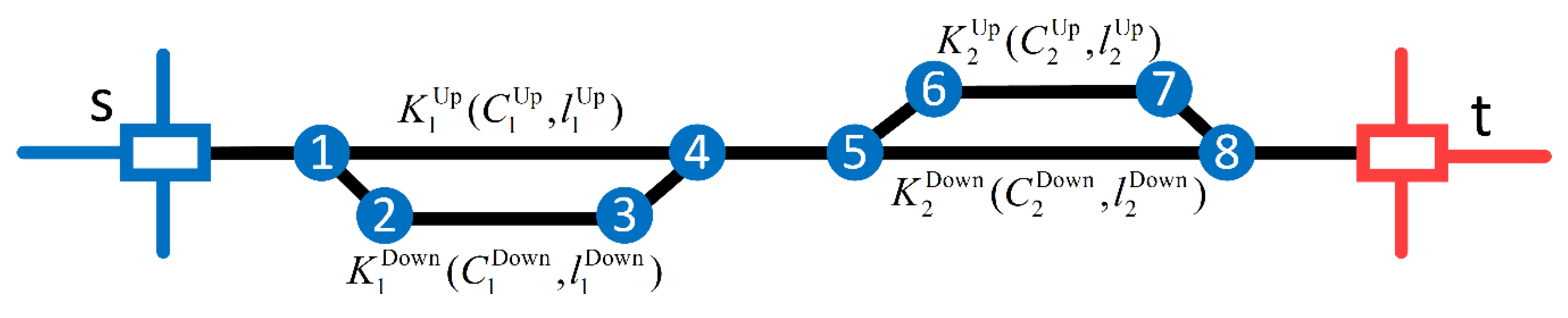
To facilitate the description of the problem, a simplified rail network with two loops is designed, as shown in Figure 2.
In this figure, let the loading area be , the unloading area be , the first loop be , and the second loop be . Respectively, let and represent the upper and lower arcs of the first loop, and let and represent the upper and lower arcs of the second loop. The capacities of these four arcs are represented by ,,, and , and their lengths are represented by ,,, and (, ), respectively.
We now give three examples to illustrate the ideas and questions we are interested in. Assumed that there are three train flows that originated from loading areas denoted as (the orang line), (the cyan line), and (the purple line), and three situations should be taken into consideration.
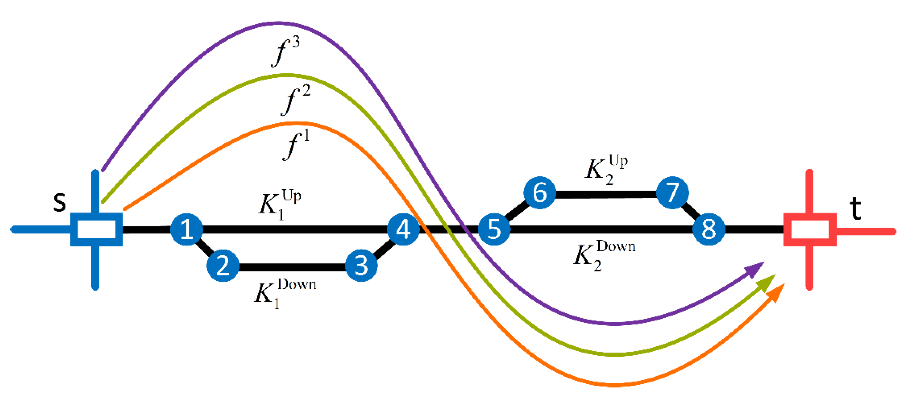
Situation 1: The capacity (the ‘capacity’ in this article refers to the residual capacity after deducting other trains that are not formed at the loading area on the rail network) of both the upper arc and lower arc of each loop can meet the needs of all train flows. In this case, these three flows (i.e., train flows) will be distributed to the rail network according to their shortest paths, as shown in Figure 3.
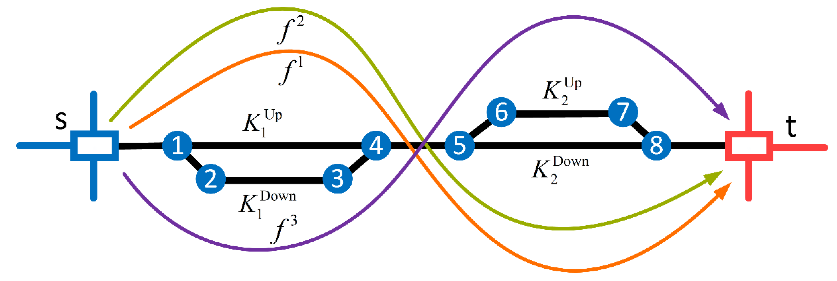
Situation 2: It may not be possible to satisfy the needs of all train flows only through the upper or lower arc of each loop, but the total capacity of the upper and lower arcs of each loop is big enough. Under this circumstance, some train flows are preferentially distributed to the arcs in the shortest path. Then, the remaining flows are distributed to the other arc. As shown in Figure 4, when and are distributed to the shortest path, the remaining capacity of and cannot accommodate , so can only be distributed to and .
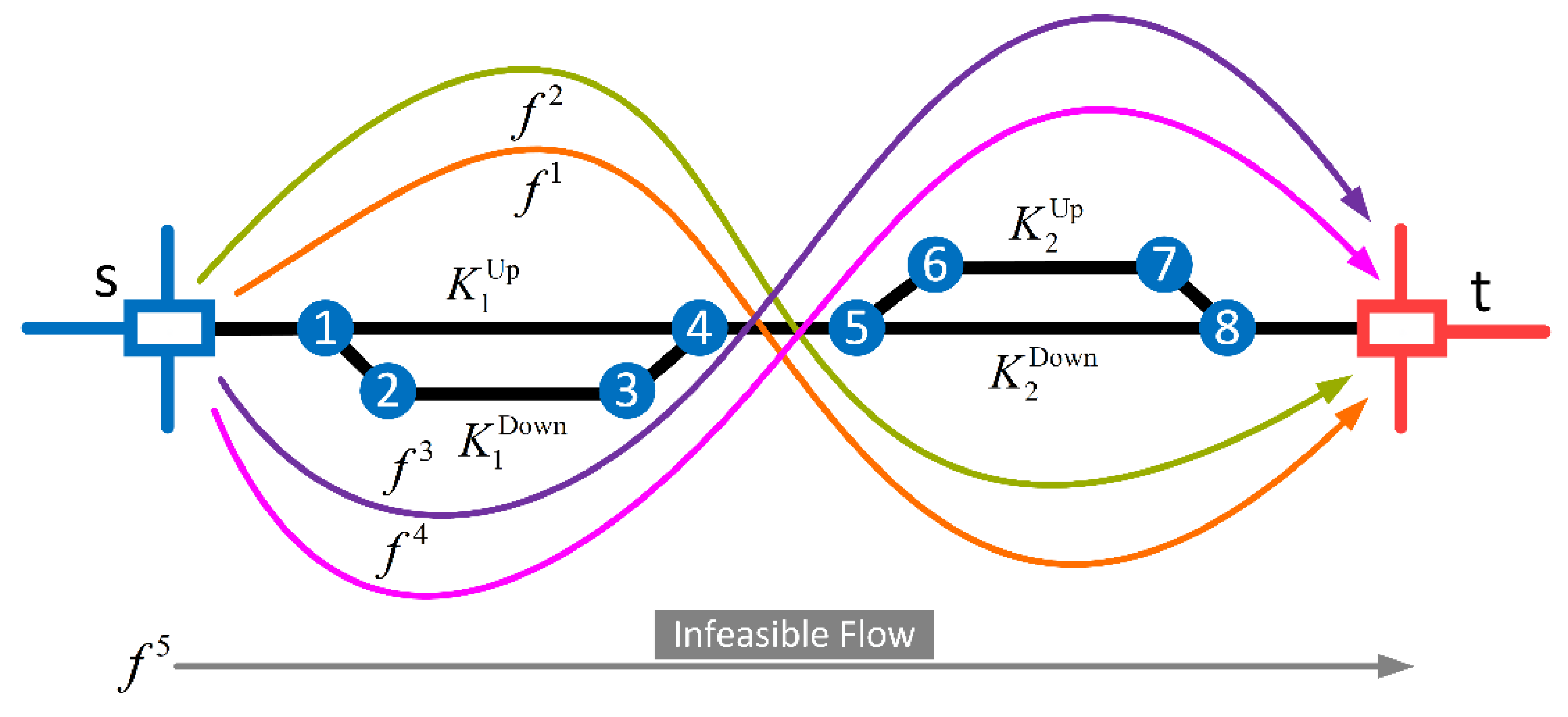
Situation 3: This situation occurs when a certain loop becomes the bottleneck of the rail network. In this case, the loop cannot accommodate all the train flows, even if the capacity of the upper and lower arcs is summed up. The flows whose demands are not satisfied are called infeasible flows. As shown in Figure 5, two more train flows, i.e., (the pink line) and (the gray line), are added to the network based on Figure 4. The best case is that both flows ( and ) can be shipped to their destinations. Unfortunately, the capacity of the rail network is insufficient to accommodate both and . Figure 5 shows that only is transported to its destination, so becomes an infeasible flow.
The above three cases correspond to different conditions for shipping trains in the multi-loop rail network; each of these conditions needs to be discussed separately. In the next section, different mathematical models will be established to solve the problem of the train’s path.
4. Mathematical Models
4.1. Variables and Parameters
Firstly, we define a rail network , where ={,,…,} represents the set of loops in the network; ={,,…,} represents the set of upper arcs, and ={,,…,} represents the set of lower arcs. is defined as the loading area, is defined as the unloading area, and the set ={, ,…,} represents the trains from to . The generalized operation cost includes salary costs, vehicle taxes, insurance, maintenance, and kilometer taxes. Since this paper is concerned with long-term planning, a parameter is introduced to represent the generalized unit operation cost to make the object function clearer.
The subscripts are defined as follows:
: Index of loops, .
: Index of train flows, .
Parameters:
: Generalized operation cost
: Incomes for transporting goods
: Profits for transporting goods
: The freight volume of the -th train flow
: Freight rate No.1 of the -th train flow(basic rate, ¥/Ton)
: Freight rate No.2 of the -th train flow(additional rate, ¥/Ton-km)
: Generalized unit operation cost
: Length of the upper arc of the -th loop
: Length of the lower arc of the -th loop
: Capacity of the upper arc of the -th loop
: Capacity of the lower arc of the -th loop
Variables:
.
It is worth noting that freight rates may vary from one good to another. According to the Rules Relating to Railway Goods Tariff, the freight rate of goods transported by rail consists of two parts, freight rate No. 1 and freight rate No. 2. The freight rate is used to calculate the freight train service fees charged by railway companies to shippers, and it depends on the goods being shipped (e.g., for grain and coal, freight rate No. 1 is 9.6 ¥/ton and freight rate No. 2 is 0.0484 ¥/ton-km; for steel, freight rate No. 1 is 10.4 ¥/ton and freight rate No. 2 is 0.0549 ¥/ton-km). The calculation formula of freight train service fees is as follows:
where is the freight rate No. 1 and is the freight rate No .2. represents the volume of freight, indicates the travel distance of the freight carried by train, and is the fees charged by railway companies to shippers.
According to the analysis in Section 2, two models can be constructed corresponding to Situation 1 (the capacity of the upper or lower arc of each loop can meet the needs of all train flows), Situation 2 (the total capacity of the upper and lower arcs can meet the needs of all train flows), and Situation 3 (the bottleneck of the rail network cannot satisfy the needs of all train flows).
4.2. Mathematical Models under Situation 1 and Situation 2
Situation 1 and Situation 2 can be summarized as one situation where the capacity of a rail network can satisfy all the requirements, so they can be solved by one mathematical model.
Assumptions:
- The capacity of a network can meet the demands of all train flows;
- A single train flow cannot be split during the itinerary.
Model I is constructed with the goal of maximizing the total profit from delivering all the train flows under the capacity constraint of each arc. 0–1 variables are introduced to indicate whether the upper arc or lower arc is selected.
Model I:
Generalized transportation cost:
Income for transporting goods:
Profits from transporting goods:
The mathematical model under Situation 1 and Situation 2 can be stated as follows:
such that
Constraints (6) and (7), respectively, indicate that the total freight volume of train flows in the upper (or lower) arc should not exceed the capacity of the upper (or lower) arc. Constraint (8) indicates that the -th train flow can only select the upper or lower arc of the -th loop, which demonstrates the principle that a single train flow cannot be split.
4.3. Mathematical Mode under Situation 3
For Situation 3, a new model should be established because of infeasible train flows. When the model is built under the condition that the capacity of a rail network cannot meet all the requirements, the decision variables should not only indicate whether the train flow selects the upper arc or the lower arc in the loop, but also whether the train flow is infeasible or not. Thus, Model I is no longer applicable.
In this case, we can introduce as a decision variable to indicate whether the train flow selects the upper arc, and introduce as another decision variable to indicate whether the train flow selects the lower arc. Then, we add a logical constraint so that each train flow can only select one arc in a loop if it is infeasible. Model II under Situation 3 is as follows:
Model II:
Generalized transportation cost:
Income for transporting goods:
The mathematical model under Situation 3 can be stated as follows:
such that
Note that:
.
Constraints (12) and (13), respectively, indicate that the total freight volume of train flows through the upper/lower arc should not exceed the capacity of the upper/lower arc. Constraint (14) indicates that a train flow can only select the upper or lower arc if it is feasible, which demonstrates the principle that a single train flow cannot be split. Constraint (15) indicates that infeasible train flows should not pass through any arc in the network, while feasible train flows should be shipped from the loading area to the unloading area. Constraint (16) indicates that the decision variables are 0–1 variables.
5. Computational Experiments
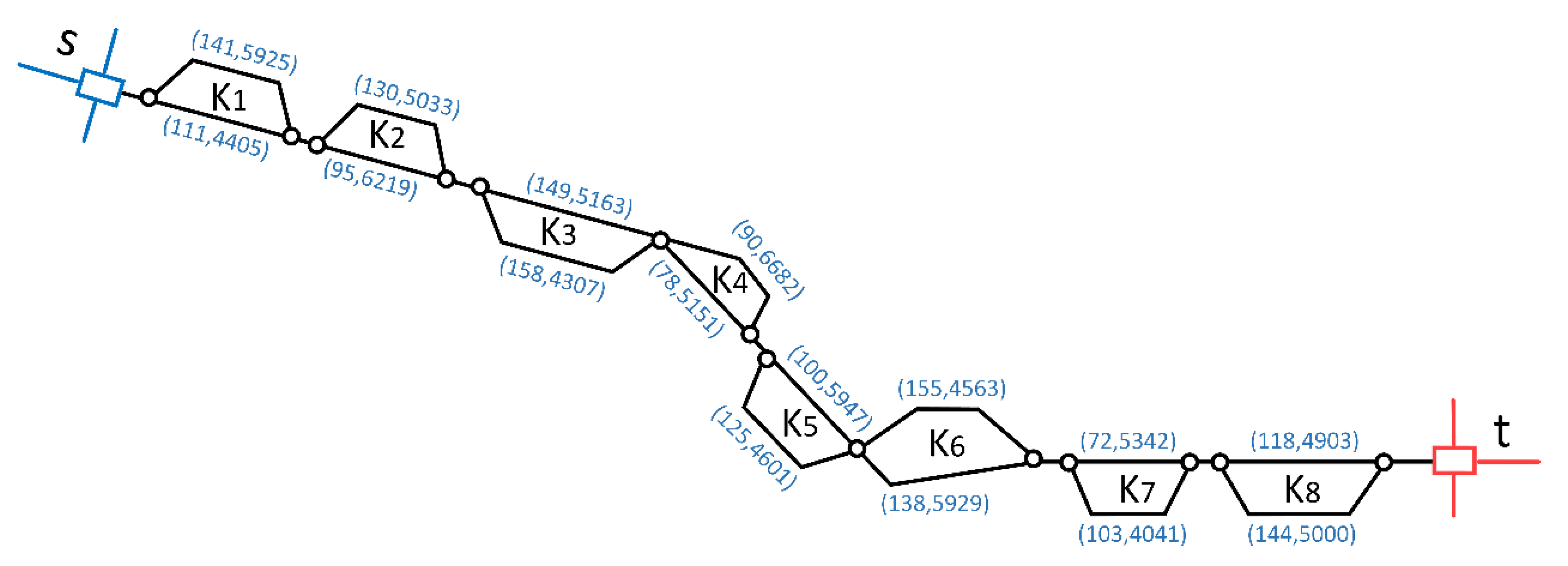
We assume that a freight multi-loop rail network (as shown in Figure 6) exists with eight loops, and the distance from loading area to unloading area is around 1000 km (for practical purposes).
In parentheses, the first number before the comma is the length of arcs, in km, and the other number after the comma is the capacity of the corresponding arcs, in 104 Tons/Year.
Computational experiments are conducted to verify the feasibility of the models in Section 3. The parameters of the rail network are shown in Table 2:
Of the upper arcs, the longest distance is 149 km (the third loop). The shortest distance is 72 km (the seventh loop). The maximum capacity is 66.82 million tons per year (the fourth loop). The minimum capacity is 45.63 million tons per year (the sixth loop). The average distance of these eight loops is around 119 km. The average capacity of these eight loops is about 54.44 million tons per year. Similarly, Of the lower arcs, the longest distance is 158 km (the third loop). The shortest distance is 78 km (the fourth loop). The maximum capacity is 62.19 million tons per year (the second loop). The minimum capacity is 40.41 million tons per year (the seventh loop). The average distance of these eight loops is around 119 km, and the average capacity of these eight loops is approximately 49.56 million tons per year.
30 train flows are also generated and their parameters are shown in Table 3:
Among the 30 flows, the largest volume flow is (4970 thousand tons per year), while the smallest is (1110 thousand tons per year), and the average volume of these 30 flows is approximately 3056 thousand tons per year. There are six different freight rates for the 30 flows, i.e., (5.7, 0.0336), (6.4, 0.0378), (7.6, 0.0435), (9.6, 0.0484), (10.4, 0.0549), and (14.8, 0.0765).
5.1. The Results of the Two Models under Situation 1 and Situation 2
In theory, both Situation 1 and Situation 2 can be solved by Model I and Model II. We make an assumption that the generalized unit operation cost is 0.04, i.e., ¥/ton-km. Firstly, Model I and Model II are tested in Lingo using the branch and bound algorithm, with the assumption that the capacity of the rail network can satisfy all requirements. The optimal solution is described in Table 4.
For Model I and Model II, we find that the solution results, which include the value of the objective function (¥147,846) and path selection (see Table 4) of each freight flow, are exactly the same, which shows that Model I and Model II can achieve the same solution.
5.2. Comparison the Solution Time between Model I and Model II under Situation 1 and Situation 2
Since both Model I and Model II can solve the problem of train flow path selection under Situation 1 and Situation 2 and can achieve a consistent result, in the next step, we focus on which model is faster or more efficient.
In this section, we use the business solution software Lingo to test the influence of train flow numbers and network loops on the performance of the aforementioned models. In this example, the number of total train flows varies from 10 to 70 and the number of loops varies from 4 to 16. It is worth noting that this test is carried out under conditions of Situation 1 and Situation 2, as Model I is not appropriate under Situation 3. The maximum solution time is set up to 24 hours and the results of solution times are shown in Table 5. In this table, the numbers in parentheses in the second column are the number of train flows and the number of loops, respectively (e.g., (30,8) represents 30 train flows and 8 loops).
It is clear that the solution time of Model I is much shorter than that of Model II. For instance, when the number of the train flow is 50 and the number of the loop is 8, the solution time is 1 second for Model I and 28 seconds for Model II. As shown in Table 5, for Model II, the solution times increases with the number of train flows and loops, because, as the number of train flows or loops increases, there may be more conflicts between different train flows. For Model I, the number of train flows and the number of loops have little effect on the solving speed, and the solving speed of Model I performed very well in the given train flows and loops. Since Model II has more decision variables and constrains than Model I under the same circumstances, it may take us more time to find an optimal solution with Model II, but the final results of both models are identical. Generally, the solution time in Model II is longer than that in Model I. However, since the studied problem is intended for planning with a long time horizon, Model II is still reasonable.
5.3. Analysis of the Solution Efficiency of Model II under Situation 3
Since only Model II can solve the path selecting problem under Situation 3, its solution efficiency will be the focus of our next study. When the capacity of the rail network is changed, it creates a problem of train path selection under Situation 3. The details are as follows (see Table 6):
Compared with the capacity in Table 2, the capacity of the third loop in Table 6 has changed from 51.63 million tons per year to 41.63 million tons per year. The third loop of the rail network becomes a bottleneck for the train flows, which remain unchanged.
We keep the generalized unit transportation cost unchanged and then test Model II by also using the branch and bound algorithm. The objective function is ¥146,257, and the optimal solution is described in Table 7.
It can be found from Table 7 that when the capacity of the third loop is reduced by 10 million tons per year, three flows with a total volume of 7.05 million tons become infeasible flows, namely, ,, and . In practice, these infeasible flows should be distributed to another route beyond the corridor.
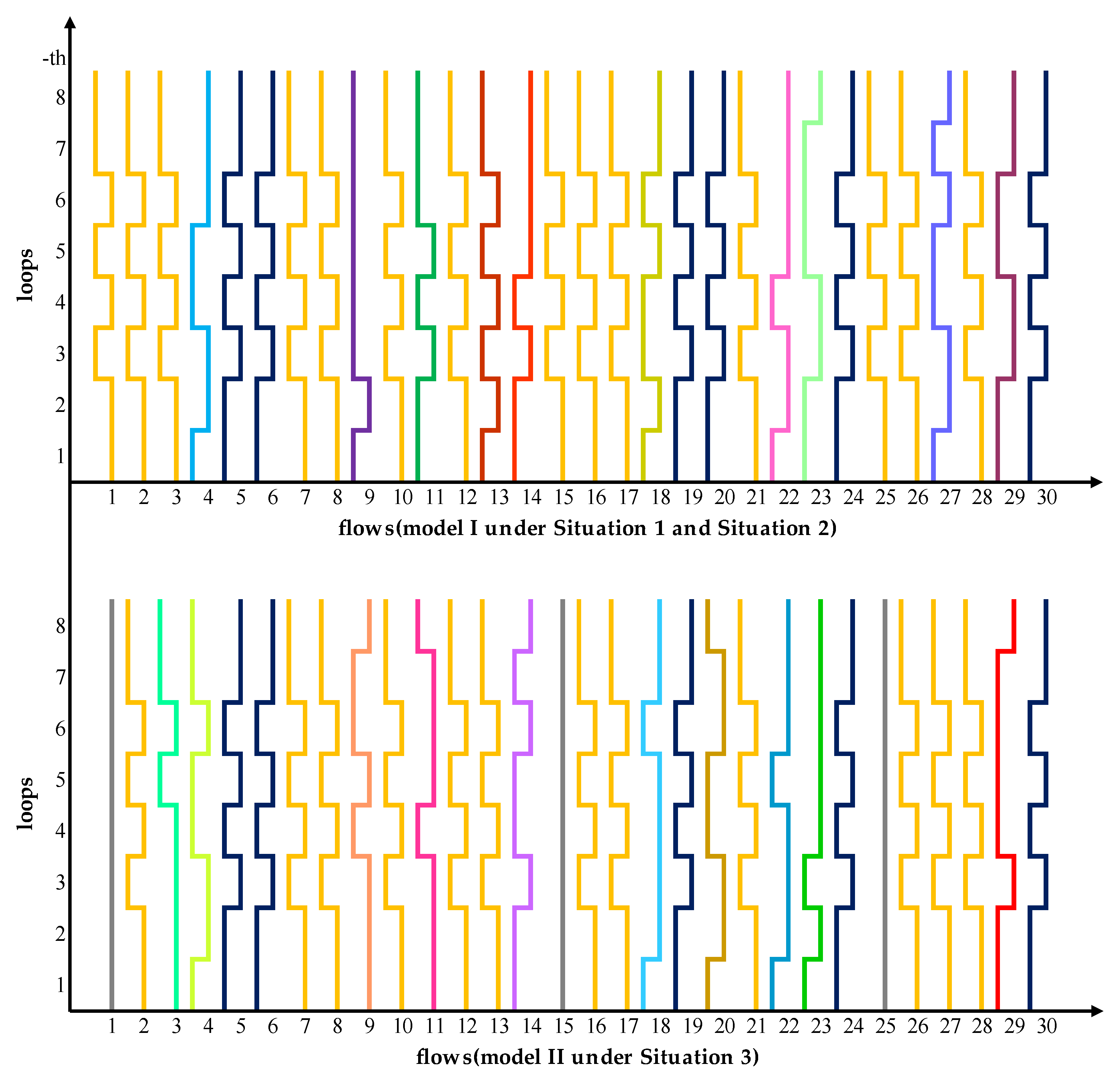
We plot the results of the above examples in Figure 7. The horizontal axis indicates the serial number of the train flows, while the vertical axis indicates the serial number of the loop in the rail network, and each broken line represents a flow. When the broken line turns to the right, it means that the flow selects the upper arc when passing through this loop. Conversely, if the broken line turns to the left, it indicates that the path selects the lower arc. The lines with the same color in the figure indicate that they have the same path. Particularly, the gray straight line represents infeasible flows.
It is clearly illustrated in Figure 7 that although the conditions of the rail network have changed, the paths of the 15 flows remain unchanged. The 15 train flows are as follows:
.
Note that there are 10 flows in the above mentioned 15 train flows share the same path: →→→→→→→→→. Coincidentally, the shortest path form → in the rail network is also →→→→→→→→→, which shows that under these two models, train flows always prefer the shortest path, followed by the other paths. In practice, the most cost-effective and shortest path always has priority in distributing flows, and then other paths are selected, which could explain why so many flows choose the shortest path.
We then enumerate the solution times of Model II under different train flows and loops. Like Section 5.2, we set the maximum solution time to 24 hours, and the results of the solution times are shown in Table 8.
As shown in Table 8, the solution time increases with the number of train flows and loops for Model II under Situation 3. However, we found that the model could not be solved within 24 hours when the number of train flows increased to 40. The result above exposes a shortcoming of Model II—when the number of the train flows increases, Lingo cannot solve the routing problem in a short time. Thus, the next task is to design a heuristic algorithm to solve the problem of large-scale train flow path selection.
5.4. A Genetic Algorithm for Solving this Problem
The path selection of a train flow (8 loops) can be expressed as follows (for Model II):
where the top and bottom lines represent the upper and lower arcs, respectively. The arc is selected when the corresponding number is 1; otherwise, it is 0. For example, the path for the train flow above is →→→→→→→→→. Since the structure of the solution of this problem is similar to the coding strategy of a genetic algorithm (GA), we try to use a genetic algorithm to solve the problem of large-scale train flow path selection.
Genetic algorithms are a part of evolutionary computing, which was inspired by Darwin’s theory of evolution. The principles and process of GAs are well known. A GA starts with a set of solutions, called a population. Solutions from parent population are taken and used to form a child population. Solutions are selected according to their fitness—the more suitable they are, the more chances they have to reproduce. By means of continuous selection, crossover, and mutation operations, the genes of a certain offspring can meet the requirements. the flowchart of the GA workflow for this problem is shown in Figure 8.
Here are some key steps to note:
We set the population size to 100 and chose the best population in a set of 500 initial solutions to generate the first population. The fitness criterion is defined as maximizing the profits for transporting goods. Roulette wheel selection is used to select candidates for parents. A fixed mutation rate of 1% is used to prevent premature convergence. An elite retention strategy, that the worst individuals in the current generation will be replaced by the elite individuals from the previous generation, is adopted.
Some details about crossover need to be explained. Crossover selects genes from parent chromosomes and creates a new offspring. For each train flow randomly selected from an individual, the process of crossover randomly chooses a crossover point, and every number before this point is copied from a parent train flow. Then, every number after the crossover point is copied from the other parent train flow. Crossover can be defined as follows (see Figure 9) (| is the crossover point):
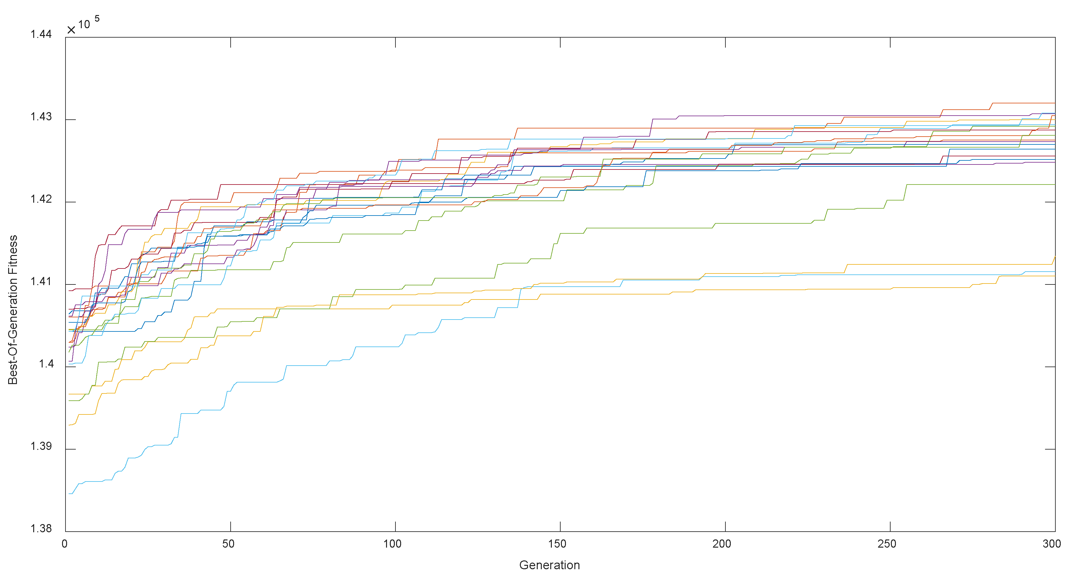
The GA above is adopted to test its feasibility with the same data in Section 5.3. We have done 20 experiments on this algorithm, and the computational results are shown in Figure 10.
In Figure 10, most of the experiments converge to around ¥142,500 and only a few experiments show poor results, which indicates the stability of the algorithm. Note that the objective function solving by the GA is ¥143,223, which decreased by 2.07% compared to ¥146,257 in Section 5.3. Therefore, we can conclude that although the GA cannot achieve an exact solution, it can approach an exact solution very well.
Next, we will analyze the solution time of the GA. We enumerate the solution times of the GA under different train flows and loops. The results of the solution times are shown in Table 9.
In Table 9, the solution time of the GA increases with the number of train flows and loops. Once set, the number of loops remains unchanged (8 loops), and the solution time is 41.5 seconds for the number of train flows to be 10 but 339.4 seconds for 70 train flows. For each additional 10 flows, the average increase of the solution time is about 50 seconds. Then the number of flows (30 flows) were kept constant to test the influence of the number of loops in the solution time. We can see that the solution time is 129 seconds when the number of loops is 4 and is 182.1 seconds when the number of loops is 16. The average increase of the solution time is about 8 seconds for each additional 2 loops.
Compared with the solution time using Lingo (as shown in Table 8), GA’s solution time increases more gradually. Moreover, it is ideal to use GA to solve the problem of selecting large-scale train flow paths (e.g., if the number of flows is 40 or more) in a short time.
To summarize, both Model I and Model II can solve the problem of train flow path selection under Situation 1 and Situation 2 and can achieve a consistent result. However, the solution time of Model I is much shorter than that of Model II. Since Lingo cannot solve Model II under Situation 3 in a short time when the scale of the train flows becomes large genetic algorithm was designed and performs well.
6. Conclusions and Future Work
In this paper, we investigate the problem of optimizing the path of trains formed at the loading area in a multi-loop rail network. Essentially, this is a combinatorial optimization problem. The complexity of the problem increases exponentially with the growth of the loop number. Three different situations are analyzed in detail. Then, two mathematic models, i.e., Model I (based on Situation 1 and Situation 2; the capacity of rail network is sufficient) and Model II (based on Situation 3; the capacity of rail network is insufficient) are established. Finally, a set of computational experiments are conducted to verify the feasibility of the models. In the experiment with 8 loops and 30 train flows, we find that Model I and Model II can achieve the same solution under Situation 1 and Situation 2. Then, the solution time between Model I and Model II under Situation 1 and Situation 2 is compared, which shows that Model I is much better than Model II. Since Model II cannot be solved by Lingo in a short time under Situation 3 when it becomes a large-scale problem, a genetic algorithm is proposed. This algorithm performs well in a set of numerical experiments. To conclusion, Lingo is recommended to be used in the case of Situation 1 and Situation 2 or the small-scale experiment of Situation 3, while GA is more suitable to solve the problem of a large-scale train flow path selection under Situation 3.
Certainly, much work remains to be done before our model can be efficiently used in the real world. Since we only consider the paths of trains formed at the loading area in this paper, all flows go through the entire network and none flow from intermediate locations. In future work, the train flows generated from intermediate stations can be taken into account. Further analysis of some terms in the objective function, and their constraints, are required, as well as a more accurate and efficient algorithm used in the solution process.
However, we have developed two adaptable models for optimizing the path of trains formed at the loading area in a multi-loop rail network, along with an efficient genetic algorithm. The results of this study should prove to be a valuable approach for the strategic management of rail freight transportation systems.
Author Contributions
The authors contributed equally to this work.
Acknowledgments
This work was supported by the National Key R&D Program of China (2018YFB1201402).
Conflicts of Interest
The authors declare no conflict of interest.
References
- Lin, B.L.; Zhu, S.N.; Chen, Z.S.; Peng, H. The 0–1 integer programming model for optimal car routing problem and algorithm for the available set in rail network. J. China Railw. Soc. 1997, 1, 9–14. [Google Scholar] [CrossRef]
- Jiang, N.; Li, X.M.; Zhu, Y.H.; Wei, C.Y. Mathematical problems in car flow routing. China Railw. Sci. 2004, 25, 121–124. [Google Scholar] [CrossRef]
- Wang, B.H.; He, S.W.; Song, R.; Wang, B. Stochastic dependent-chance programming model and hybrid genetic algorithm for car flow routing plan. J. China Railw. Soc. 2007, 29, 6–11. [Google Scholar] [CrossRef]
- Nong, J.; Ji, L.; Ye, Y.L.; Liu, Z.J. Distributed algorithm for the optimization of railway car flow routing. China Railw. Sci. 2008, 29, 115–121. [Google Scholar] [CrossRef]
- Cao, X.M.; Wang, X.F.; Lin, B.L. Collaborative optimization model of the loaded & empty car flow routing and the empty car distribution of multiple car types. China Railw. Sci. 2009, 30, 114–118. [Google Scholar] [CrossRef]
- Sadykov, R.; Lazarev, A.; Shiryaev, V.; Stratonnikov, A. Solving a freight railcar flow problem arising in Russia. In 13th Workshop on Algorithmic Approaches for Transportation Modelling, Optimization, and Systems, Proceedings of the ATMOS ’13, Sophia Antipolis, France, 5 September 2013; Dagstuhl: Wadern, Germany, 2013; pp. 55–67. [Google Scholar] [CrossRef]
- Borndörfer, R.; Fügenschuh, A.; Klug, T.; Schang, T.; Schlechte, T.; Schülldorf, H. The Freight Train Routing Problem; Konrad-Zuse-Zentrum für Informationstechnik Berlin: Berlin, Germany, 2014. [Google Scholar]
- Borndörfer, R.; Fügenschuh, A.; Klug, T.; Schang, T.; Schlechte, T.; Schülldorf, H. The freight train routing problem for congested railway networks with mixed traffic. Transp. Sci. 2016, 50, 408–423. [Google Scholar] [CrossRef]
- Zhao, C.; Yang, L.X.; Li, S.K. Allocating freight empty cars in railway networks with dynamic demands. Discret. Dyn. Nat. Soc. 2014. [Google Scholar] [CrossRef]
- Wen, X.H.; Lin, B.L.; Chen, L. Optimization model of railway vehicle flow routing based on tree form. J. China Railw. Soc. 2016, 38, 1–6. [Google Scholar] [CrossRef]
- Fu, L.; Dessouky, M. Algorithms for a special class of state-dependent shortest path problems with an application to the train routing problem. J. Sched. 2018, 1–20. [Google Scholar] [CrossRef]
- Brucker, P.; Hurink, J.; Rolfes, T. Routing of railway carriages. J. Glob. Optim. 2003, 27, 313–332. [Google Scholar] [CrossRef]
- Fügenschuh, A.; Homfeld, H.; Schülldorf, H. Single-car routing in rail freight transport. Transp. Sci. 2013, 49, 130–148. [Google Scholar] [CrossRef]
- Assad, A.A. Modelling of rail networks: Toward a routing/makeup model. Transp. Res. Part B: Methodol. 1980, 14, 101–114. [Google Scholar] [CrossRef]
- Haghani, A.E. Formulation and solution of a combined train routing and makeup, and empty car distribution model. Transp. Res. Part B Methodol. 1989, 23, 433–452. [Google Scholar] [CrossRef]
- Lin, B.L.; Zhu, S.N. Synthetic optimization of train routing and makeup plan in a railway network. J. China Railw. Soc. 1996, 18, 1–7. [Google Scholar] [CrossRef]
- Yan, Y.S.; Hu, Z.A.; Li, X.Y. Comprehensive optimization of train formation plan and wagon-flow path based on fluctuating wagon-flow. J. Transp. Syst. Eng. Inf. Technol. 2017, 4, 019. [Google Scholar] [CrossRef]
- Cominetti, R.; Correa, J. Common-lines and passenger assignment in congested transit networks. Transp. Sci. 2001, 35, 250–267. [Google Scholar] [CrossRef]
- Fu, H.L.; Sperry, B.R.; Nie, L. Operational impacts of using restricted passenger flow assignment in high-speed train stop scheduling problem. Math. Probl. Eng. 2013. [Google Scholar] [CrossRef]
- Zhou, F.; Shi, J.G.; Xu, R.H. Estimation method of path-selecting proportion for urban rail transit based on AFC data. Math. Probl. Eng. 2015. [Google Scholar] [CrossRef]
- Xu, Y.; Jia, B.; Ghiasi, A.; Li, X.P. Train routing and timetabling problem for heterogeneous train traffic with switchable scheduling rules. Transp. Res. Part C Emerg. Technol. 2017, 84, 196–218. [Google Scholar] [CrossRef]
- Wang, Y.; Gao, Y.; Yu, X.Y.; Hansen, I.A.; Miao, J.R. Optimization models for high-speed train unit routing problems. Comput. Ind. Eng. 2018. [Google Scholar] [CrossRef]
- Samà, M.; Pellegrini, P.; D’Ariano, A.; Rodriguez, J.; Pacciarelli, D. Ant colony optimization for the real-time train routing selection problem. Transp. Res. Part B: Methodol. 2016, 85, 89–108. [Google Scholar] [CrossRef]
- Samà, M.; D’Ariano, A.; Pacciarelli, D.; Corman, F. Lower and upper bound algorithms for the real-time train scheduling and routing problem in a railway network. IFAC-Pap 2016, 49, 215–220. [Google Scholar] [CrossRef]
- Kou, W.H.; Li, Z.P. Maximum flow distributing algorithm under restricted capacity condition at transportation network sites. J. Transp. Eng. Inf. 2008, 42, 639–665. [Google Scholar] [CrossRef]
- Kou, W.H.; Li, Z.P. Maximum flow assignment algorithm for transshipment nodes with flow demands in transportation network. J. Southwest Jiaotong Univ. 2009, 44, 118–121. [Google Scholar] [CrossRef]
- Bakó, A.; Hartványi, T.; Szüts, I. Transportation network realization with an optimization method. In Proceedings of the 2009 4th International Symposium on Computational Intelligence and Intelligent Informatics, Luxor, Egypt, 21–25 October 2009; pp. 81–84. [Google Scholar] [CrossRef]
- Gao, Q.P. A Minimum cost and maximum flow model of hazardous materials transportation. Adv. Mater. Res. 2011, 305, 363–366. [Google Scholar] [CrossRef]
- Singh, V.K.; Tripathi, I.K.; Nimisha, N. Applications of maximal network flow problems in transportation and assignment problems. J. Math. Res. 2010, 2. [Google Scholar] [CrossRef]
- Di, Z.; Yang, L.X.; Qi, J.G.; Gao, Z.Y. Transportation network design for maximizing flow-based accessibility. Transp. Res. Part B Methodol. 2018, 110, 209–238. [Google Scholar] [CrossRef]
Figure 1.
Situations from one loop to loops.

Figure 2.
A toy network with two loops .

Figure 3.
Distribution of train flows for Situation 1.

Figure 4.
Distribution of train flows for Situation 2.

Figure 5.
Distribution of train flows for Situation 3.

Figure 6.
A rail network for computational experiments.

Figure 7.
Comparison of the results of Model I and Model II.

Figure 8.
Flowchart of the genetic algorithm (GA) workflow.

Figure 9.
A toy example of crossover.

Figure 10.
Twenty computational experiments for Model II under Situation 3.


Table 1.
A literature review of some classic studies.
| No. | Author | Model | Solution Technique | ||
|---|---|---|---|---|---|
| Model Structure | Decision Variables | Constraints | |||
| 1 | Haghani (1989) | MINLP | Integer variables | a) Capacity constraint | A heuristic decomposition technique |
| 2 | Lin et al. (1997) | ILP | 0–1 variables | a) Operation principle b) Capacity constraint | Simulated annealing algorithm |
| 3 | Borndörfer et al. (2016) | MINLP | 0–1 variables | a) Capacity constraint b) Time constraint | Linearization of the objective function |
| 4 | Sadykov et al. (2013) | LP | 0–1 and integer variables | a) Operation principle b) Capacity constraint | A column generation approach |
| 5 | Fügenschuh et al. (2013) | MINLP | 0–1 and integer variables | a) Operation principle b) Capacity constraint | Tree-based reformulation and heuristic cuts |
| 6 | Samà et al. (2016) | ILP | 0–1 variables | a) Operation principle | Ant colony optimization |
MINLP indicates Mixed-Integer Nonlinear Programming, ILP indicates Integer Linear Programming and LP indicates Linear Programming.
Table 2.
Parameters of the rail network.
| No. | Name | Distance (up) (Km) | Distance (down) (Km) | Capacity (up) (104 Tons/Year) | Capacity (down) (104 Tons/Year) |
|---|---|---|---|---|---|
| 1 | 141 | 111 | 5925 | 4405 | |
| 2 | 130 | 95 | 5033 | 6219 | |
| 3 | 149 | 158 | 5163 | 4307 | |
| 4 | 90 | 78 | 6682 | 5151 | |
| 5 | 100 | 125 | 5947 | 4601 | |
| 6 | 155 | 138 | 4563 | 5929 | |
| 7 | 72 | 103 | 5342 | 4041 | |
| 8 | 118 | 144 | 4903 | 5000 |
Table 3.
Parameters of the train flows.
| No. | Name | Volume (104 Tons/Year) | Freight rate No. 1 (¥/Ton) | Freight rate No. 2 (¥/Ton-km) |
|---|---|---|---|---|
| 1 | 241 | 5.7 | 0.0336 | |
| 2 | 381 | 6.4 | 0.0378 | |
| 3 | 111 | 7.6 | 0.0435 | |
| 4 | 375 | 9.6 | 0.0484 | |
| 5 | 285 | 10.4 | 0.0549 | |
| 6 | 186 | 14.8 | 0.0765 | |
| 7 | 251 | 6.4 | 0.0378 | |
| 8 | 213 | 7.6 | 0.0435 | |
| 9 | 216 | 9.6 | 0.0484 | |
| 10 | 481 | 7.6 | 0.0435 | |
| 11 | 137 | 9.6 | 0.0484 | |
| 12 | 462 | 6.4 | 0.0378 | |
| 13 | 182 | 7.6 | 0.0435 | |
| 14 | 326 | 9.6 | 0.0484 | |
| 15 | 128 | 5.7 | 0.0336 | |
| 16 | 192 | 6.4 | 0.0378 | |
| 17 | 194 | 7.6 | 0.0435 | |
| 18 | 399 | 9.6 | 0.0484 | |
| 19 | 483 | 10.4 | 0.0549 | |
| 20 | 342 | 9.6 | 0.0484 | |
| 21 | 477 | 7.6 | 0.0435 | |
| 22 | 475 | 9.6 | 0.0484 | |
| 23 | 226 | 9.6 | 0.0484 | |
| 24 | 427 | 14.8 | 0.0765 | |
| 25 | 336 | 6.4 | 0.0378 | |
| 26 | 402 | 7.6 | 0.0435 | |
| 27 | 205 | 9.6 | 0.0484 | |
| 28 | 497 | 7.6 | 0.0435 | |
| 29 | 377 | 9.6 | 0.0484 | |
| 30 | 162 | 10.4 | 0.0549 |
Table 4.
The results for Model I and Model II.
| No. | Name | Paths |
|---|---|---|
| 1 | →→→→→→→→→ | |
| 2 | →→→→→→→→→ | |
| 3 | →→→→→→→→→ | |
| 4 | →→→→→→→→→ | |
| 5 | →→→→→→→→→ | |
| 6 | →→→→→→→→→ | |
| 7 | →→→→→→→→→ | |
| 8 | →→→→→→→→→ | |
| 9 | →→→→→→→→→ | |
| 10 | →→→→→→→→→ | |
| 11 | →→→→→→→→→ | |
| 12 | →→→→→→→→→ | |
| 13 | →→→→→→→→→ | |
| 14 | →→→→→→→→→ | |
| 15 | →→→→→→→→→ | |
| 16 | →→→→→→→→→ | |
| 17 | →→→→→→→→→ | |
| 18 | →→→→→→→→→ | |
| 19 | →→→→→→→→→ | |
| 20 | →→→→→→→→→ | |
| 21 | →→→→→→→→→ | |
| 22 | →→→→→→→→→ | |
| 23 | →→→→→→→→→ | |
| 24 | →→→→→→→→→ | |
| 25 | →→→→→→→→→ | |
| 26 | →→→→→→→→→ | |
| 27 | →→→→→→→→→ | |
| 28 | →→→→→→→→→ | |
| 29 | →→→→→→→→→ | |
| 30 | →→→→→→→→→ |
Table 5.
The solution times comparing Model I and Model II.
| No. | Parameters | Model I | Model II | No. | Parameters | Model I | Model II |
|---|---|---|---|---|---|---|---|
| 1 | (10,8) | < 1 s | < 1 s | 8 | (30,4) | 1 s | < 1 s |
| 2 | (20,8) | < 1 s | < 1 s | 9 | (30,6) | 1 s | < 1 s |
| 3 | (30,8) | 1 s | 3 s | 10 | (30,10) | 1 s | 3 s |
| 4 | (40,8) | 1 s | 24 s | 11 | (30,12) | 1 s | 3 s |
| 5 | (50,8) | 1 s | 28 s | 12 | (30,14) | 1 s | 6 s |
| 6 | (60,8) | 1 s | 154 s | 13 | (30,16) | 1 s | 16 s |
| 7 | (70,8) | 1 s | 275 s |
Table 6.
Parameters of the rail network based on Table 2.
Table 6.
Parameters of the rail network based on Table 2.
| No. | Name | Distance (up) (Km) | Distance (down) (Km) | Capacity (up) (104 Tons/Year) | Capacity (down) (104 Tons/Year) |
|---|---|---|---|---|---|
| 1 | 141 | 111 | 5925 | 4405 | |
| 2 | 130 | 95 | 5033 | 6219 | |
| 3 | 149 | 158 | 4163 | 4307 | |
| 4 | 90 | 78 | 6682 | 5151 | |
| 5 | 100 | 125 | 5947 | 4601 | |
| 6 | 155 | 138 | 4563 | 5929 | |
| 7 | 72 | 103 | 5342 | 4041 | |
| 8 | 118 | 144 | 4903 | 5000 |
Table 7.
The results for Model II.
| No. | Name | Paths |
|---|---|---|
| 1 | — | |
| 2 | →→→→→→→→→ | |
| 3 | →→→→→→→→→ | |
| 4 | →→→→→→→→→ | |
| 5 | →→→→→→→→→ | |
| 6 | →→→→→→→→→ | |
| 7 | →→→→→→→→→ | |
| 8 | →→→→→→→→→ | |
| 9 | →→→→→→→→→ | |
| 10 | →→→→→→→→→ | |
| 11 | →→→→→→→→→ | |
| 12 | →→→→→→→→→ | |
| 13 | →→→→→→→→→ | |
| 14 | →→→→→→→→→ | |
| 15 | - | |
| 16 | →→→→→→→→→ | |
| 17 | →→→→→→→→→ | |
| 18 | →→→→→→→→→ | |
| 19 | →→→→→→→→→ | |
| 20 | →→→→→→→→→ | |
| 21 | →→→→→→→→→ | |
| 22 | →→→→→→→→→ | |
| 23 | →→→→→→→→→ | |
| 24 | →→→→→→→→→ | |
| 25 | - | |
| 26 | →→→→→→→→→ | |
| 27 | →→→→→→→→→ | |
| 28 | →→→→→→→→→ | |
| 29 | →→→→→→→→→ | |
| 30 | →→→→→→→→→ |
Table 8.
The solution times of Model II under Situation 3.
| No. | Parameters | Solution Times | No. | Parameters | Solution Times |
|---|---|---|---|---|---|
| 1 | (10,8) | < 1 s | 8 | (30,4) | 3 s |
| 2 | (20,8) | < 1 s | 9 | (30,6) | 4 s |
| 3 | (30,8) | 5 s | 10 | (30,10) | 5 s |
| 4 | (40,8) | > 24 h | 11 | (30,12) | 21 s |
| 5 | (50,8) | > 24 h | 12 | (30,14) | 35 s |
| 6 | (60,8) | > 24 h | 13 | (30,16) | 44 s |
| 7 | (70,8) | > 24 h |
Table 9.
The solution times of the GA.
| No. | Parameters | Solution Times | No. | Parameters | Solution Times |
|---|---|---|---|---|---|
| 1 | (10,8) | 41.5 s | 8 | (30,4) | 129 s |
| 2 | (20,8) | 107.1 s | 9 | (30,6) | 134.6 s |
| 3 | (30,8) | 135.9 s | 10 | (30,10) | 153.1 s |
| 4 | (40,8) | 216.2 s | 11 | (30,12) | 159.3 s |
| 5 | (50,8) | 254.4 s | 12 | (30,14) | 169.8 s |
| 6 | (60,8) | 326.1 s | 13 | (30,16) | 182.1 s |
| 7 | (70,8) | 380.9 s |
© 2019 by the authors. Licensee MDPI, Basel, Switzerland. This article is an open access article distributed under the terms and conditions of the Creative Commons Attribution (CC BY) license (http://creativecommons.org/licenses/by/4.0/).
Share and Cite
MDPI and ACS Style
Li, X.; Lin, B.; Zhao, Y. Optimizing the Paths of Trains Formed at the Loading Area in a Multi-loop Rail Network. Symmetry 2019, 11, 844. https://0-doi-org.brum.beds.ac.uk/10.3390/sym11070844
AMA Style
Li X, Lin B, Zhao Y. Optimizing the Paths of Trains Formed at the Loading Area in a Multi-loop Rail Network. Symmetry. 2019; 11(7):844. https://0-doi-org.brum.beds.ac.uk/10.3390/sym11070844
Chicago/Turabian StyleLi, Xingkui, Boliang Lin, and Yinan Zhao. 2019. "Optimizing the Paths of Trains Formed at the Loading Area in a Multi-loop Rail Network" Symmetry 11, no. 7: 844. https://0-doi-org.brum.beds.ac.uk/10.3390/sym11070844
Note that from the first issue of 2016, this journal uses article numbers instead of page numbers. See further details here.