A Study on Hypergraph Representations of Complex Fuzzy Information


1
Department of Mathematics, University of the Punjab, New Campus, Lahore 54590, Pakistan
2
Department of Mathematics, Faculty of Science, King Abdulaziz University, P.O. Box 80219, Jeddah 21589, Saudi Arabia
3
BORDA Research Unit and IME, University of Salamanca, 37007 Salamanca, Spain
*
Author to whom correspondence should be addressed.
Symmetry 2019, 11(11), 1381; https://0-doi-org.brum.beds.ac.uk/10.3390/sym11111381
Submission received: 21 October 2019
/
Revised: 1 November 2019
/
Accepted: 5 November 2019
/
Published: 7 November 2019
(This article belongs to the Special Issue Symmetry and Complexity 2019)
Abstract
:The paradigm shift prompted by Zadeh’s fuzzy sets in 1965 did not end with the fuzzy model and logic. Extensions in various lines have produced e.g., intuitionistic fuzzy sets in 1983, complex fuzzy sets in 2002, or hesitant fuzzy sets in 2010. The researcher can avail himself of graphs of various types in order to represent concepts like networks with imprecise information, whether it is fuzzy, intuitionistic, or has more general characteristics. When the relationships in the network are symmetrical, and each member can be linked with groups of members, the natural concept for a representation is a hypergraph. In this paper we develop novel generalized hypergraphs in a wide fuzzy context, namely, complex intuitionistic fuzzy hypergraphs, complex Pythagorean fuzzy hypergraphs, and complex q-rung orthopair fuzzy hypergraphs. Further, we consider the transversals and minimal transversals of complex q-rung orthopair fuzzy hypergraphs. We present some algorithms to construct the minimal transversals and certain related concepts. As an application, we describe a collaboration network model through a complex q-rung orthopair fuzzy hypergraph. We use it to find the author having the most outstanding collaboration skills using score and choice values.
1. Introduction
In 1965, fuzzy sets (FSs) were originally defined by Zadeh [1] as a novel approach to represent uncertainty arising in various fields. The idea of “partial membership” was questioned by many researchers at that time. The extension of crisp sets to FSs, i.e., the extension of membership function from to , bears comparison to the generalization of to . Just like was extended to with the incorporation of imaginary quantities, FSs have been extended to complex fuzzy sets (CFSs) by Ramot et al. [2]. A CFS is characterized by a membership function whose range is not limited to [0,1] but extends to the unit circle in the complex plane. Hence, is a complex-valued function that assigns a grade of membership of the form , to any element x in the universe of discourse. The membership function of CFS consists of two terms, namely, an amplitude term which lies in the unit interval and a phase term (periodic term) which lies in the interval . During the last few years, many researchers have paid special attention to CFSs. Yazdanbakhsh and Dick [3] gives an updated review of the development of CFSs.
Atanassov [4] had proposed a different extension of FSs by intuitionistic fuzzy sets (IFSs). Fuzzy sets give the degree of membership of an element in a given set (the non-membership of degree equals one minus the degree of membership), while IFSs give both a degree of membership and a degree of non-membership, which are to some extent independent from each other. The truth (T) and falsity (F) membership functions are used to characterize an IFS in such a way that the sum of truth and falsity degrees should not be greater than one at any point. These figures allow for some indeterminacy in the expression of memberships. Progress on the investigation of IFSs and related extensions of the FS concept continues to be made. Liu et al. [5] introduced different types of centroid transformations of IF values. Feng et al. [6] defined various new operations for generalized IF soft sets. Recently, Shumaiza et al. [7] have proposed group decision-making based on the VIKOR method with trapezoidal bipolar fuzzy information. Akram and Arshad [8] proposed a novel trapezoidal bipolar fuzzy TOPSIS method for group decision-making. Alcantud et al [9] proposed a novel modelization of the party formation process, in which citizens’ private opinions are described by means of continuous fuzzy profiles. A novel hesitant fuzzy model for group decision-making was proposed by Alcantud and Giarlotta [10].
Of particular importance are two extensions of IFSs proposed by Yager [11,12,13]. In these papers he introduced Pythagorean fuzzy sets (PFSs) and q-rung orthopair fuzzy sets (q-ROFSs). A q-ROFS is characterized by means of truth and falsity degrees satisfying the constraint that the sum of the qth powers of both degrees should be less than one. PFSs consist of the case where . Thus, q-ROFSs generalize both the notions of IFSs and PFSs so that the uncertain information can be dealt with in a more widened range. After that, Liu and Wang [14] applied certain simple weighted operators to aggregate q-ROFSs in decision-making. Intertemporal choice problems have been investigated with the help of fuzzy soft sets [15]. These problems appear in the analysis of environmental issues and sustainable development with an infinitely long horizon, project evaluations, or health care [16,17]. In multi-attribute decision making, q-ROF Heronian mean operators were defined by Wei et al. [18]. For further applications of q-ROFSs, we refer the readers to the work presented in [19,20]. Complex intuitionistic fuzzy sets (CIFSs) were introduced by Alkouri and Salleh [21] in order to generalize IFSs in the spirit of [2] by adding non-membership degree to the CFSs subjected to the constraint . The CIFSs are used to handle information about uncertainty and periodicity simultaneously. As an extension of both PFSs and CIFSs, Ullah et al. [22] proposed complex Pythagorean fuzzy sets (CPFSs) and discussed some applications.
The vagueness in the representation of various objects and the uncertain interactions between them originated the necessity of fuzzy graphs (FGs), that were first defined by Rosenfeld [23] (see also the remarks made by Bhattacharya [24]). The notion of FGs was extended to complex fuzzy graphs (CFGs) by Thirunavukarasu et al. [25]. Intuitionistic fuzzy graphs (IFGs) were defined by Parvathi and Karunambigai [26]. The energy of Pythagorean fuzzy graphs (PFGs) was discussed by Akram and Naz [27]. Akram and Habib [28] defined q-ROF competition graphs and discussed their applications. Akram et al. [29] proposed a novel description on edge-regular q-ROFGs. Yaqoob et al. [30] defined complex intuitionistic fuzzy graphs (CIFGs) and discussed an application of CIFGs in cellular networks to test the proposed model. Later on, complex neutrosophic graphs were studied by Yaqoob and Akram [31]. Recently, complex Pythagorean fuzzy graphs (CPFGs) and their applications in decision making have been put forward by Akram and Naz [32].
A hypergraph, as an extension of a crisp graph, is a powerful tool to model different practical problems in various fields, including biological sciences, computer science, sustainable development and social networks [33,34,35]. Co-authorship networks, an important type of social network, have been studied extensively from various angles such as degree distribution analysis, social community extraction and social entity ranking. Most of the previous studies consider the co-authorship relation between two or more authors as a collaboration using crisp hypergraphs. Han et al. [36] proposed a hypergraph analysis approach to understand the importance of collaborations in co-authorship networks. Zhang and Liu [37] proposed a hypergraph model of social tagging networks. Ouvrard et al. [38] studied the hypergraph modeling and visualization of collaboration networks.
In order to allow for uncertainty in crisp hypergraphs, fuzzy hypergraphs (FHGs) were defined by Kaufmann [39] as an extension of FGs. Lee-Kwang and Lee [40] discussed fuzzy partitions using FHGs. A valuable contribution to FGs and FHGs has been proposed by Mordeson and Nair [41]. Fuzzy transversals of FHGs were studied by Goetschel et al. [42]. Intuitionistic fuzzy hypergraphs (IFHGs) were defined by Parvathi et al. [43]. Further discussion on IFHGs can be seen in [44,45]. Akram and Luqman [46] defined bipolar neutrosophic hypergraphs with applications. Transversals and minimal transversals of m-polar FHGs were studied by Akram and Sarwar [47]. Luqman et al. [48] presented q-ROFHGs and their applications. Further, Luqman et al. [49,50] have proposed m-polar and q-rung picture fuzzy hypergraph models of granular computing.
The proposed research generalizes the concepts of CIFGs and CPFGs. These existing models can only depict the uncertainty having periodic nature occurring in pairwise relationships. The existence of various complex network models in which the relationships are more generalized rather than the pairwise relationships motivates the extension of CIFGs and CPFGs to complex intuitionistic fuzzy and complex Pythagorean fuzzy hypergraphs. Let us consider the modeling of research collaborations through CIFGs and CPFGs. The uncertainty and periodicity of the given data are dealt with with the help of phase terms and amplitude terms, respectively. Two research articles are connected through an edge if both have the same author but if more than two articles are written by the same author then CIFGs and CPFGs fail to model this situation. Thus the main objective of this study is to generalize the concepts of CIFGS and CPFGs to complex q-rung orthopair fuzzy hypergraphs. As argued above, complex q-ROF models provide more flexibility than IFSs and FSs. Therefore a complex q-rung orthopair fuzzy hypergraph model proves to be a very general framework to deal with vagueness in complex hypernetworks when the symmetrical relationships go beyond pairwise interactions. The generality of the proposed model can be observed from the reduction of complex q-rung orthopair fuzzy models to CIF and CPF models for and , respectively. Moreover, most of the previous studies consider the co-authorship relation between two or more authors as a collaboration using crisp hypergraphs. Here we consider a complex q-rung orthopair fuzzy hypergraph model of co-authorship network to represent the collaboration relations between authors having uncertainty and vagueness of periodic nature simultaneously.
The contents of this paper are as follows. In Section 2 and Section 3, we define complex intuitionistic fuzzy hypergraphs and complex Pythagorean fuzzy hypergraphs, respectively. In Section 4, complex q-ROF hypergraphs are discussed. In Section 5, we define the q-ROF transversals and minimal transversals of q-ROF hypergraphs. Section 6 illustrates an application of q-ROF hypergraphs in research collaboration networks. We also present an algorithm to select an author with powerful collaboration characteristics using the score and choice values of q-rung orthopair fuzzy hypergraphs and give a brief comparison of our proposed model with CIF and CPF models. The final Section 7 contains conclusions and future research directions.
2. Complex Intuitionistic Fuzzy Hypergraphs
In this section, we define the notion of complex intuitionistic fuzzy hypergraphs. A complex intuitionistic fuzzy hypergraph extends the concept of CIFGs. The proposed hypergraph model is used to handle the uncertain and periodic real-life situations when the relationships are analyzed between more than two objects. The main model that we use in our research design is given in the next definition:
Definition 1.
[21] A complex intuitionistic fuzzy set (CIFS) I on the universal set Y is defined as,
where , , , and for every .
For every , and are the amplitude terms for membership and non-membership of u, and and are the phase terms for membership and non-membership of u. CIFSs where the phase terms equal zero (for all u) reduce to ordinary IFSs. When in addition, the amplitude terms for non-membership of all elements equal zero, we obtain a FS.
The application of this concept to graphs was produced in [30]. We represent definition of complex intuitionistic fuzzy graphs as follows:
Definition 2.
A complex intuitionistic fuzzy graph (CIFG) on Y is an ordered pair , where A is a complex intuitionistic fuzzy set on Y and B is complex intuitionistic fuzzy relation on Y such that,
, and , for all .
When we apply Definition 1 to hypergraphs we obtain the following structure that generalizes Definition 2:
Definition 3.
Let Y be a non-trivial set of universe. A complex intuitionistic fuzzy hypergraph (CIFHG) is defined as an ordered pair , where is a finite family of complex intuitionistic fuzzy sets on Y and is a complex intuitionistic fuzzy relation on complex intuitionistic fuzzy sets ’s such that the following conditions hold:
- (i)
- , and , for all
- (ii)
- for all
Notice that is the crisp hyperedge of .
Note that the above formula reduces to Definition 2 if we consider only two vertices in an hyperedge.
We illustrate the previous definition with a graphical example.
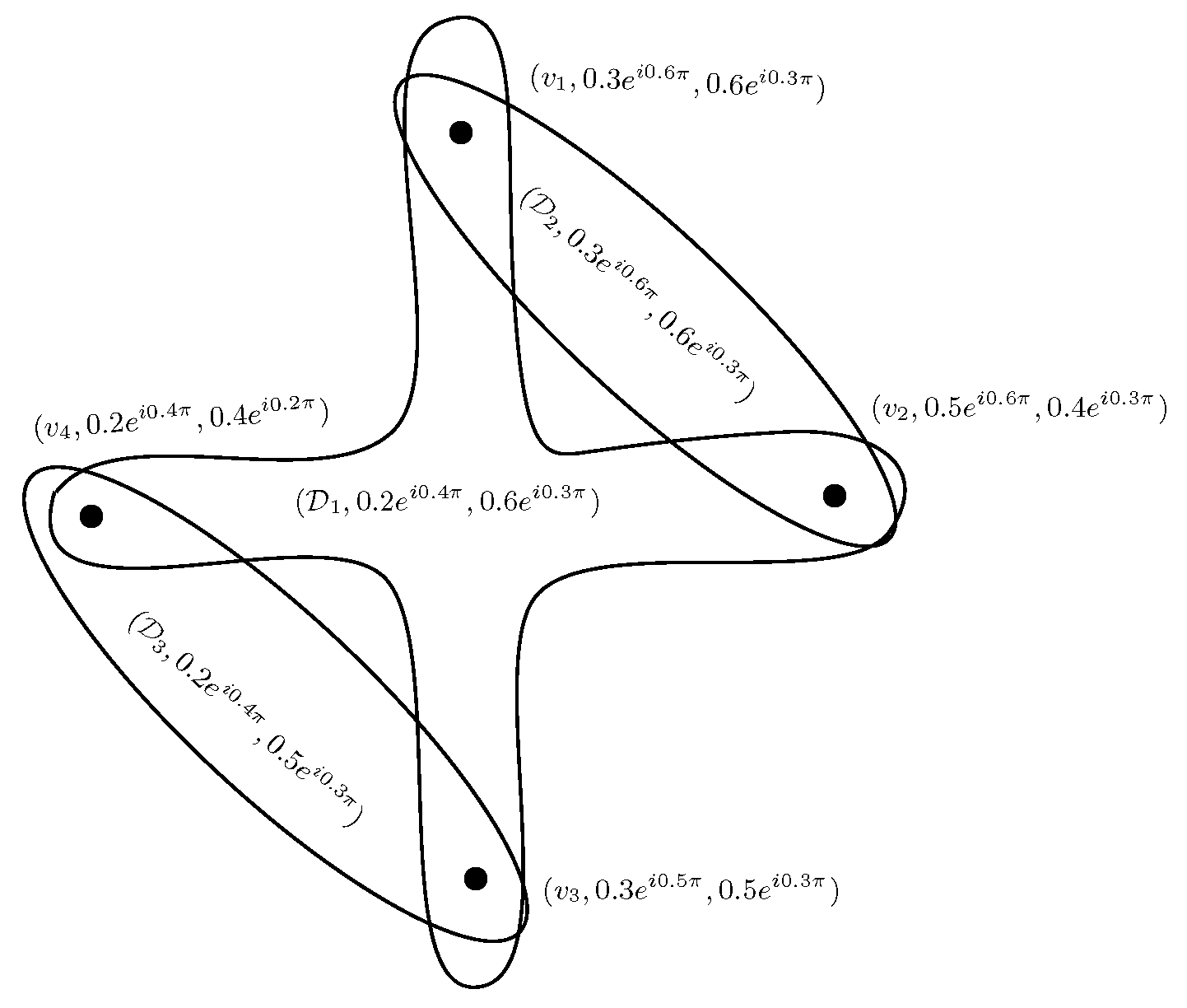
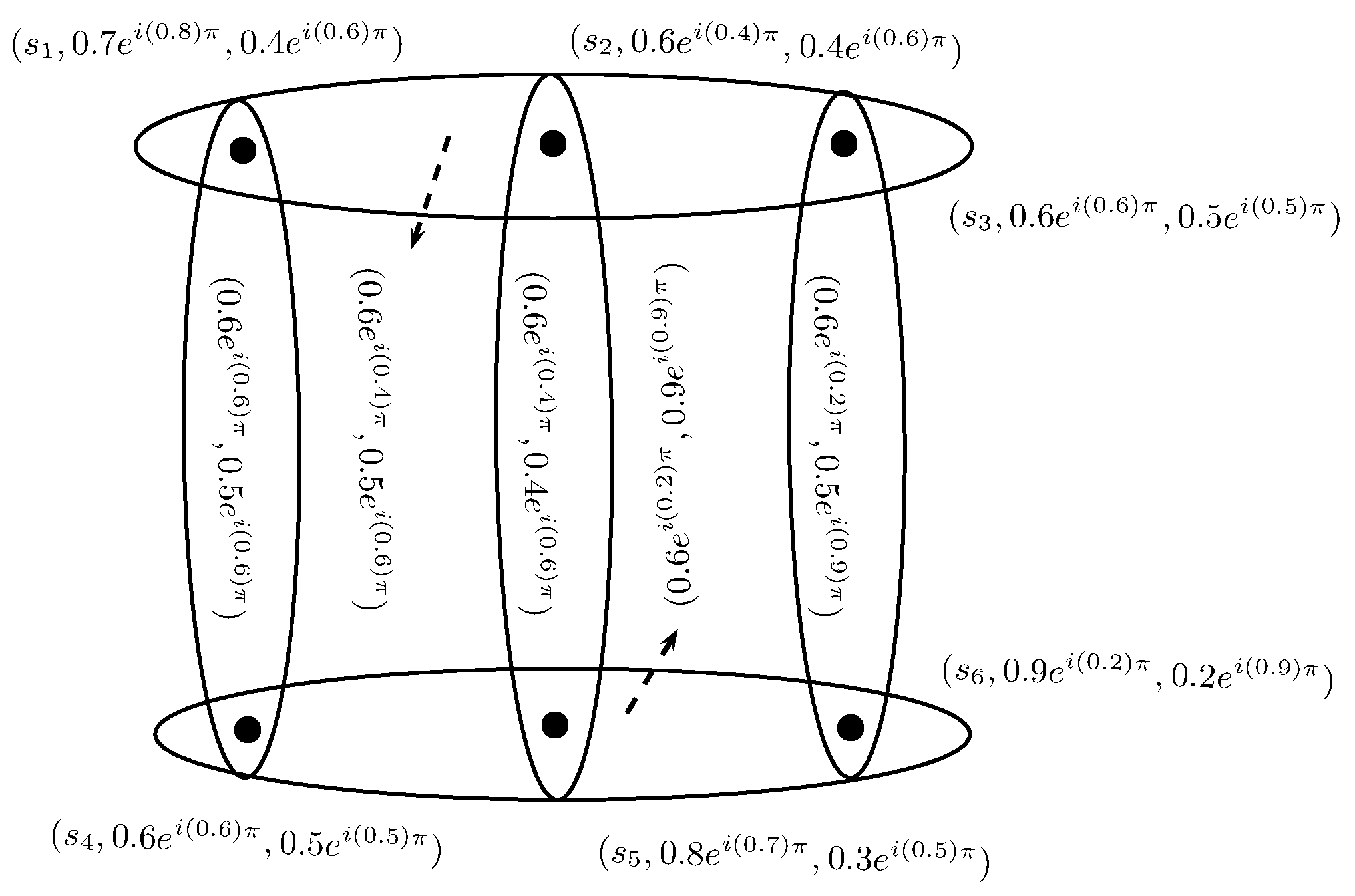
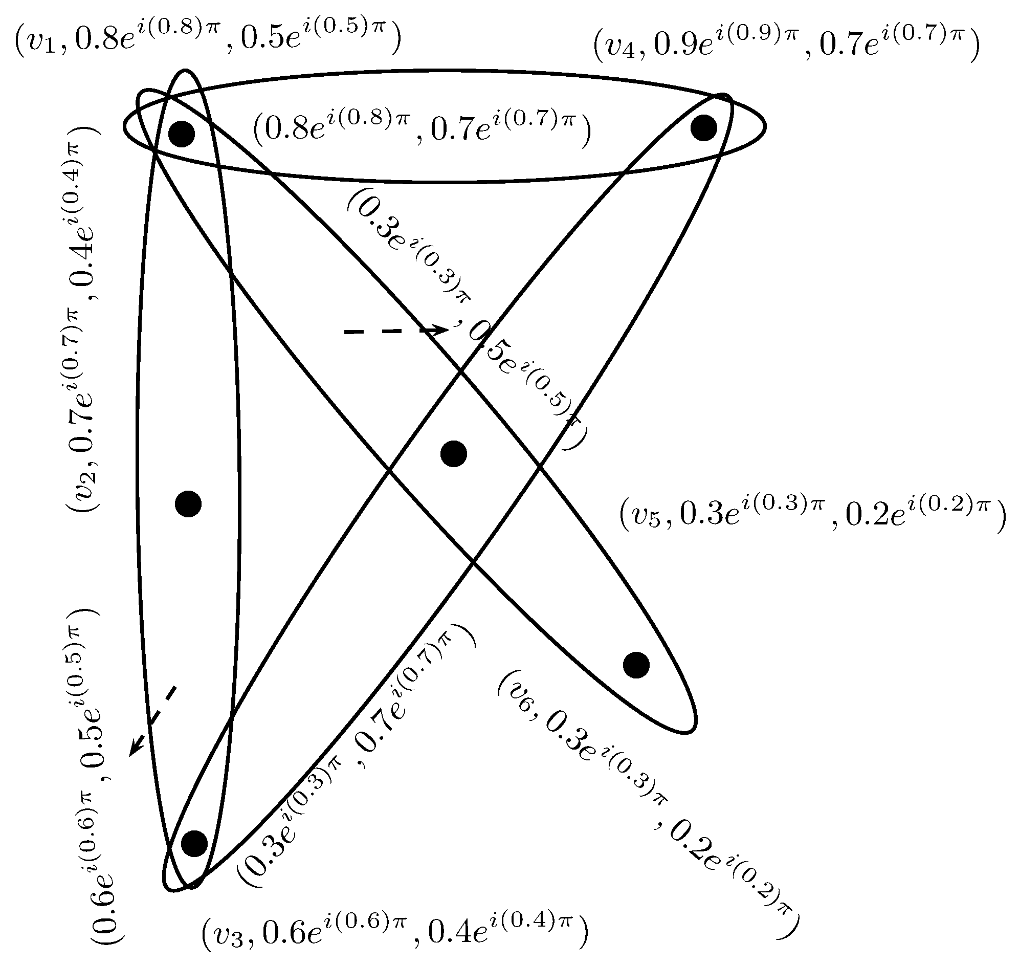
Example 1.
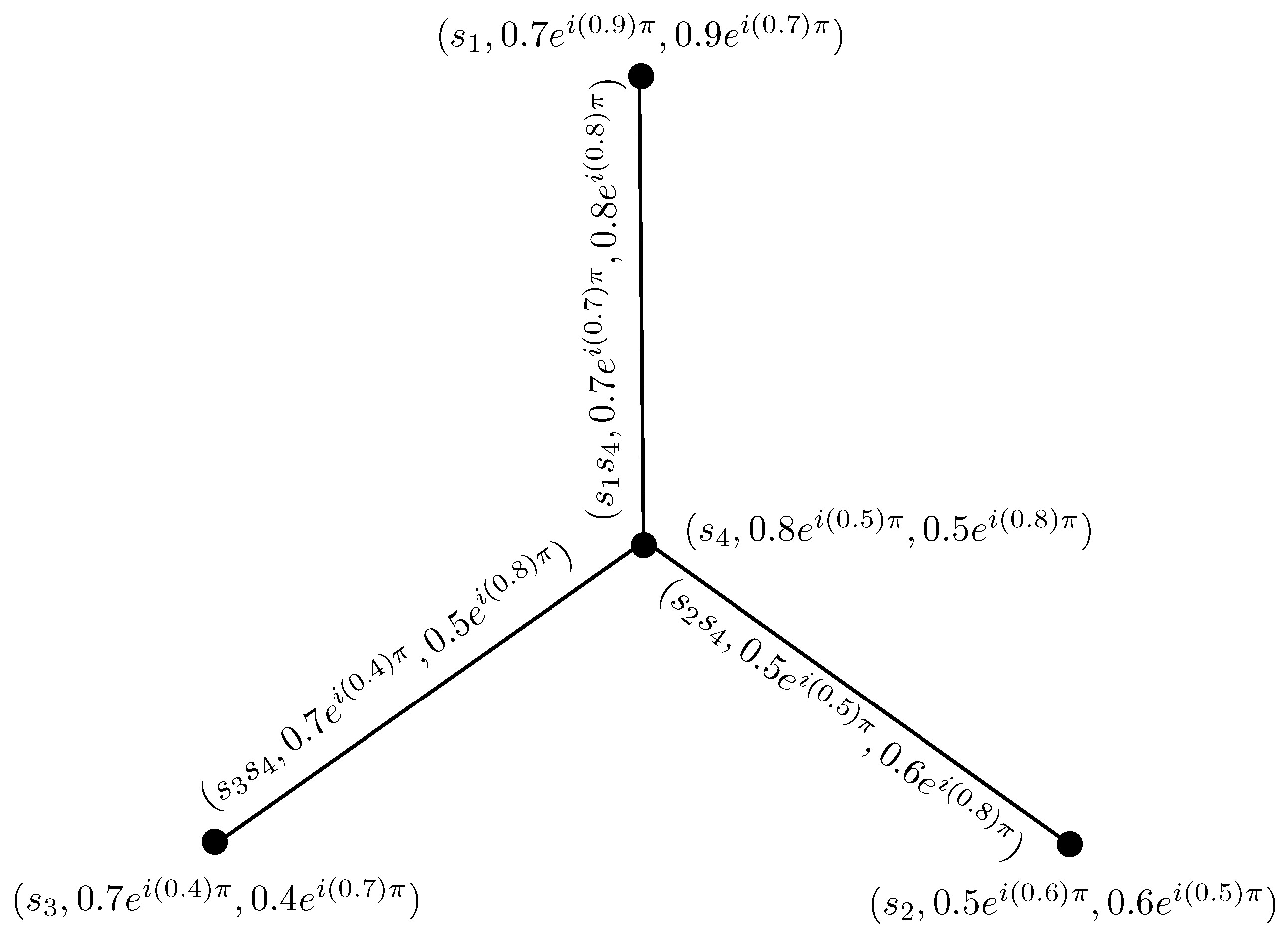
Consider a CIFHG on . The CIFR is defined as, , , and . The corresponding CIFHG is shown in Figure 1.
Simple CIFHGs are the following special types of CIFHGs:
Definition 4.
A CIFHG is simple if whenever and , then .
A CIFHG is support simple if whenever , , and , then .
Our next notion produces a link between CIFHGs and crisp hypergraphs. The subsequent example illustrates this construction.
Definition 5.
Let be a CIFHG. Suppose that and such that . The level hypergraph of H is defined as an ordered pair , where
- (i)
- and ,
- (ii)
- .
Note that the level hypergraph of H is a crisp hypergraph.
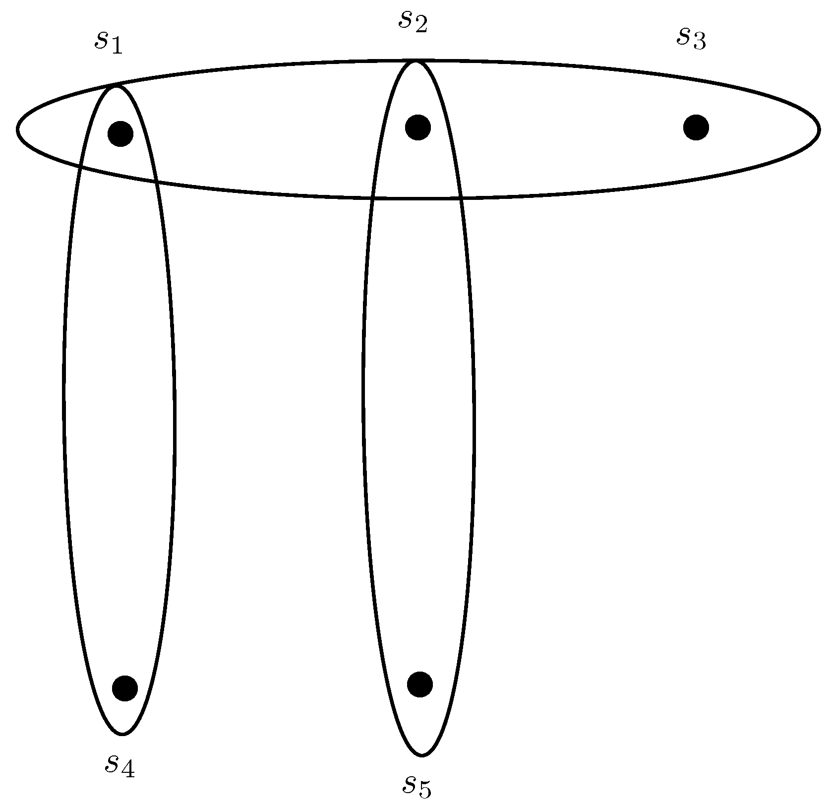
Example 2.
Definition 6.
Let be a CIFHG. The complex intuitionistic fuzzy line graph of H is defined as an ordered pair , where and there exists an edge between two vertices in if . The membership degrees of are given as,
- (i)
- ,
- (ii)
- .
Definition 7.
A CIFHG is said to be linear if for every ,
- (i)
- ,
- (ii)
- .
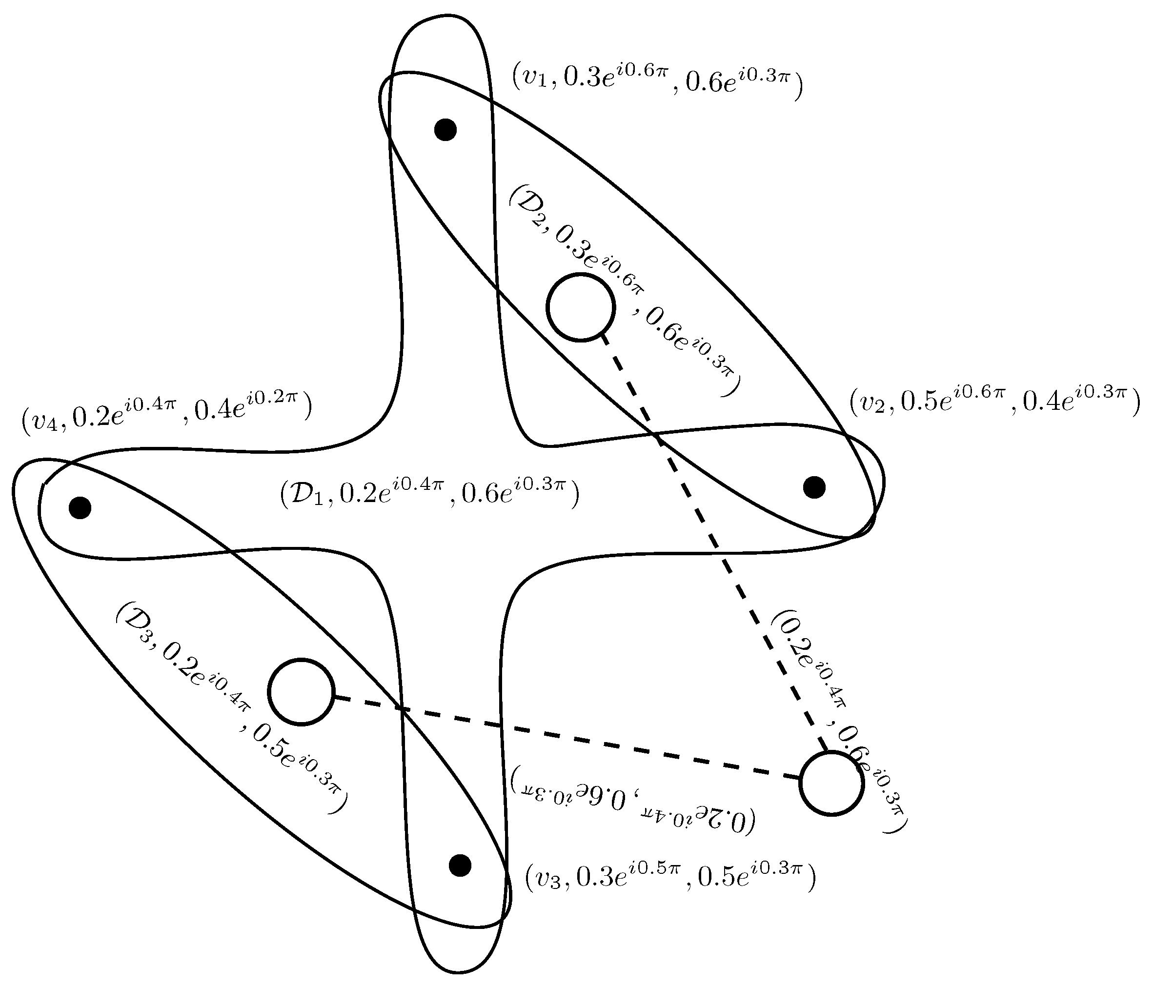
Example 3.
Consider a CIFHG as shown in Figure 1. By direct calculations, we have
Note that, and . Hence, CIFHG is not linear. The corresponding CIFHG and its line graph is shown in Figure 3.
Theorem 1.
A simple strong CIFG is the complex intuitionistic line graph of a linear CIFHG.
Definition 8.
The 2-section of a CIFHG is a CIFG having same set of vertices as that of H, is a CIFS on , and such that .
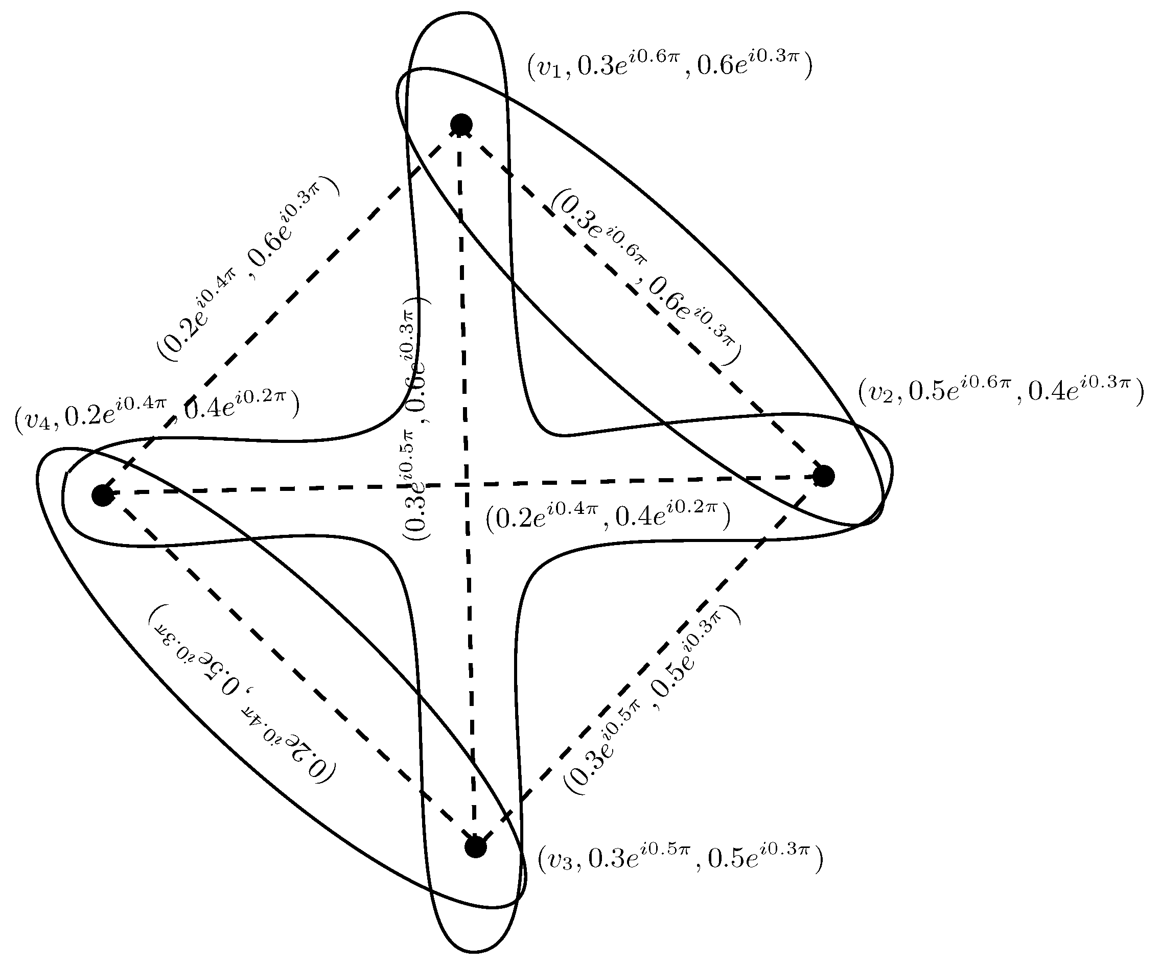
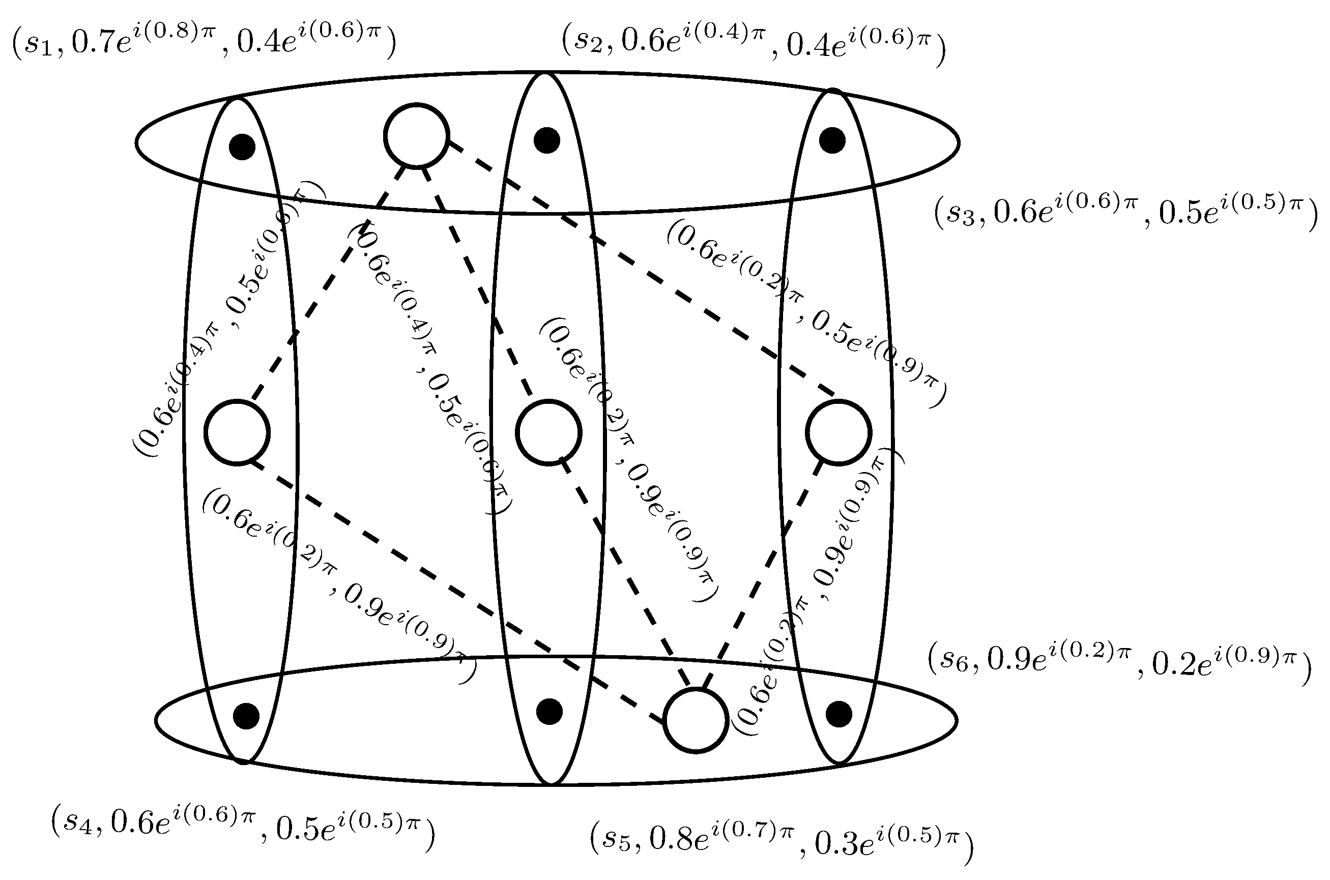
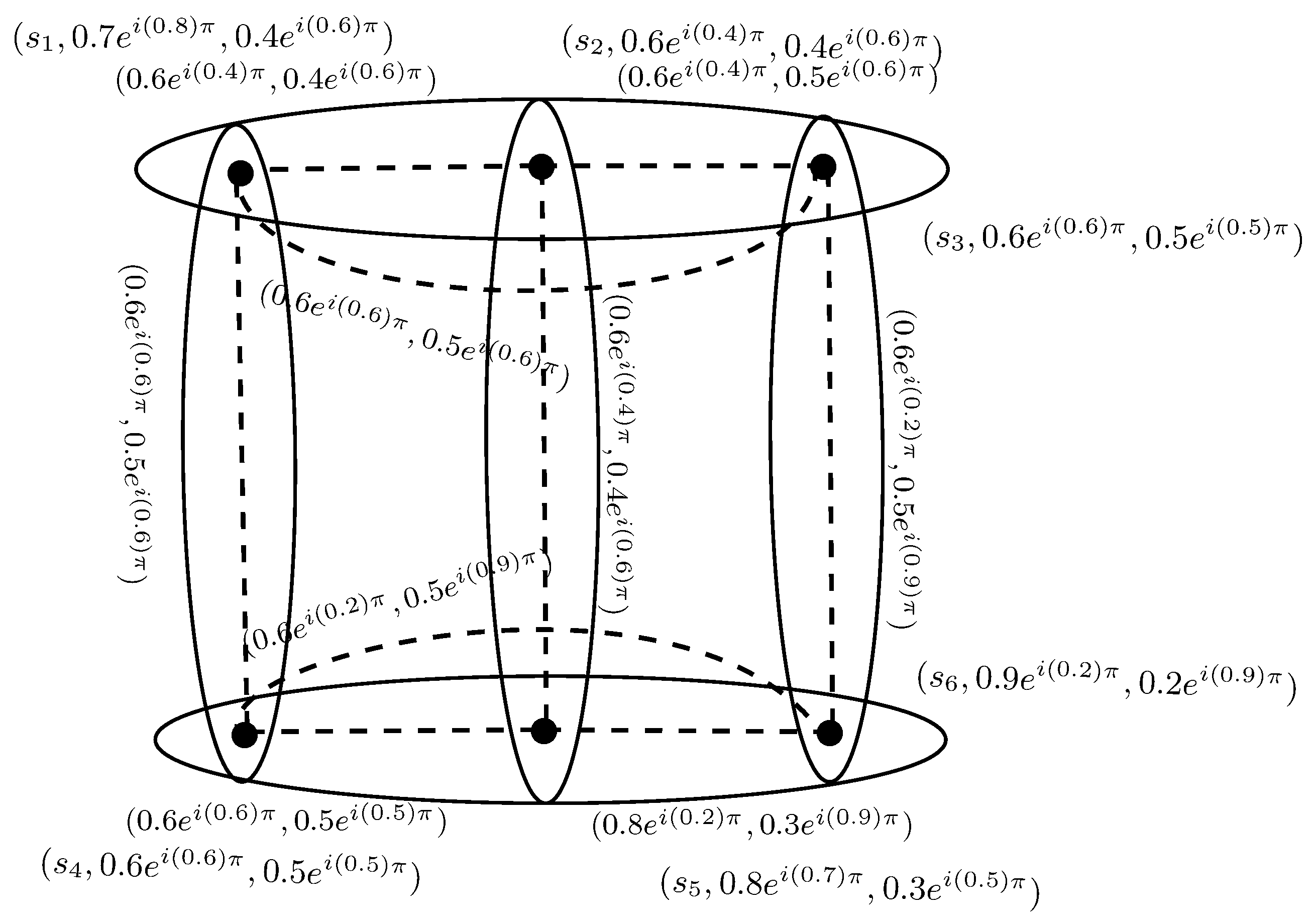
Example 4.
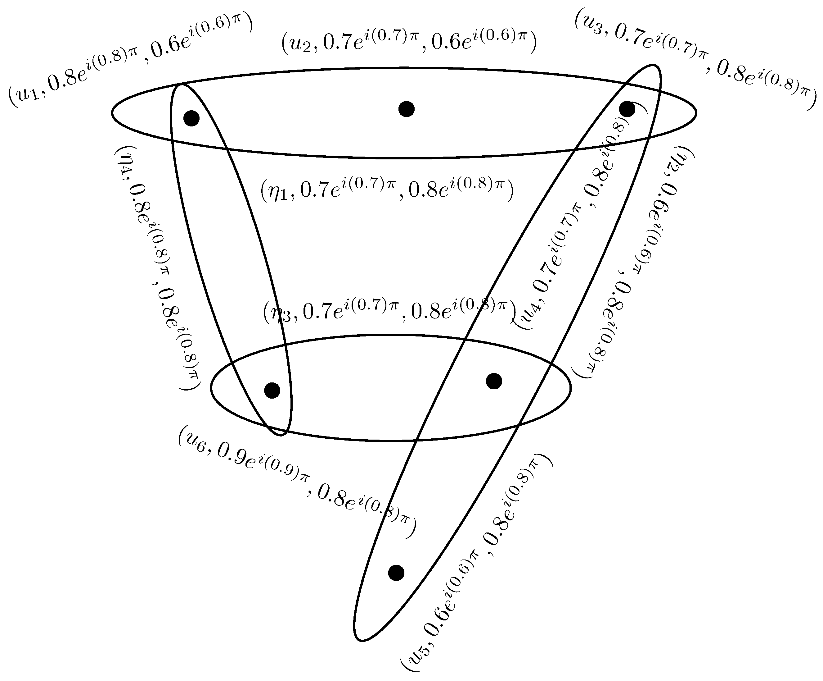
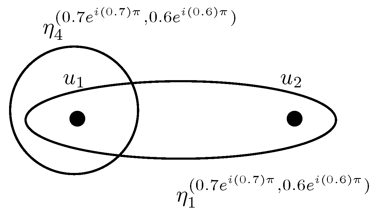
An example of a CIFHG is given in Figure 4. The 2-section of H is presented with dashed lines.
Definition 9.
Let be a CIFHG. A complex intuitionistic fuzzy transversal (CIFT) τ is a CIFs of Y satisfying the condition for all , where is the height of ρ.
A minimal complex intuitionistic fuzzy transversal t is the CIFT of H having the property that if , then τ is not a CIFT of H.
3. Complex Pythagorean Fuzzy Hypergraphs
We now turn our attention to the next class of hypergraphs called complex Pythagorean fuzzy hypergraphs. A complex Pythagorean fuzzy hypergraph is the generalization of CPFGs and CIFHGs. The occurrence of truth and falsity degrees whose sum is not less than one but the sum of squares does not exceed one in complex hypernetworks motivates the necessity of this proposed model.
Definition 10.
[32] A complex Pythagorean fuzzy graph (CPFG) on Y is an ordered pair , where C is a CPFS on Y and D is CPFR on Y such that,
, and , for all .
Definition 11.
A complex Pythagorean fuzzy hypergraph (CPFHG) on Y is defined as an ordered pair , where is a finite family of CPFSs on Y and is a CPFR on CPFSs ’s such that,
- (i)
- , and for all
- (ii)
- for all
Note that, is the crisp hyperedge of .
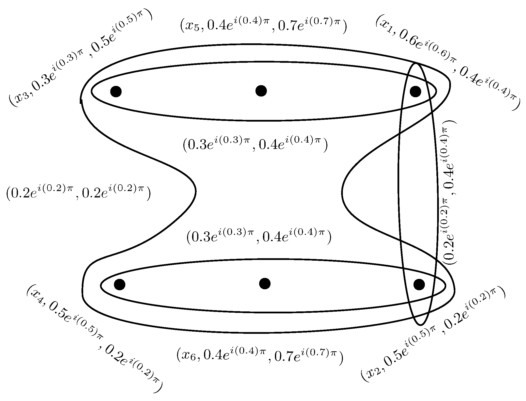
Example 5.
Consider a CPFHG on . The CPFR is defined as, , , , , and . The corresponding CPFHG is shown in Figure 5.
Definition 12.
A CPFHG is simple if whenever and , then .
A CPFHG is support simple if whenever , , and , then .
Definition 13.
Let be a CPFHG. Suppose that and such that . The level hypergraph of is defined as an ordered pair , where
- (i)
- and ,
- (ii)
- .
Note that, level hypergraph of is a crisp hypergraph.
Example 6.
Definition 14.
Let be a CPFHG. The complex Pythagorean fuzzy line graph of is defined as an ordered pair , where and there exists an edge between two vertices in if , for all . The membership degrees of are given as,
- (i)
- ,
- (ii)
- .
Definition 15.
A CPFHG is said to be linear if for every ,
- (i)
- ,
- (ii)
- .
Example 7.
Theorem 2.
A simple strong CPFG is the complex Pythagorean fuzzy line graph of a linear CPFHG.
Definition 16.
The 2-section of a CPFHG is a CPFG having same set of vertices as that of , is a CPFS on , and such that .
Example 8.
An example of a CPFHG is given in Figure 8. The 2-section of is presented with dashed lines.
Definition 17.
Let be a CPFHG. A complex Pythagorean fuzzy transversal (CPFT) τ is a CPFS of Y satisfying the condition for all , where is the height of ρ.
A minimal complex Pythagorean fuzzy transversal t is the CPFT of having the property that if , then τ is not a CPFT of .
4. Complex q-Rung Orthopair Fuzzy Hypergraphs
This section explores the class of complex q-rung orthopair fuzzy graphs and complex q-rung orthopair fuzzy hypergraphs. Complex q-rung orthopair fuzzy hypergraphs generalize the notions of CIFHGs and CPFHGs. The class of Cq-ROFSs extends the classes of CIFSs and CPFSs. The space of Cq-ROFSs increases as the value of parameter q increases. Based on these advantages of Cq-ROFSs, we combine the theories of Cq-ROFSs and graphs to define complex q-rung orthopair fuzzy graphs and complex q-rung orthopair fuzzy hypergraphs.
Definition 18.
[13] A q-rung orthopair fuzzy set (q-ROFS) Q in the universal set Y is defined as, , where the function defines the truth-membership and defines the falsity-membership of the element and for every , . Furthermore, is called the indeterminacy degree or q-ROF index of u to the set Q.
Definition 19.
A complex q-rung orthopair fuzzy set (Cq-ROFS) S in the universal set Y is given as,
where , , , and for every , .
Remark 1.
- When , C1-ROFS is called a CIFS.
- When , C2-ROFS is called a CPFS.
Definition 20.
Let and , be two Cq-ROFSs in Y, then
- (i)
- , , and , for amplitudes and phase terms, respectively, for all .
- (ii)
- , , and , for amplitudes and phase terms, respectively, for all .
Definition 21.
Let and , be two Cq-ROFSs in Y, then
- (i)
- (ii)
Definition 22.
A complex q-rung orthopair fuzzy relation (Cq-ROFR) is a Cq-ROFS in given as,
where , , characterize the truth and falsity degrees of R, and such that for all , .
Example 9.
Let be the universal set and be the subset of . Then, the C5-ROFR R is given as,
Note that, , for all Hence, R is a C5-ROFR on Y.
Definition 23.
A complex q-rung orthopair fuzzy graph(Cq-ROFG) on Y is an ordered pair , where is a complex q-rung orthopair fuzzy set on Y and is complex q-rung orthopair fuzzy relation on Y such that,
, for all .
Remark 2.
Note that,
- When , C1-ROFG is called a CIFG.
- When , C2-ROFG is called a CPFG.
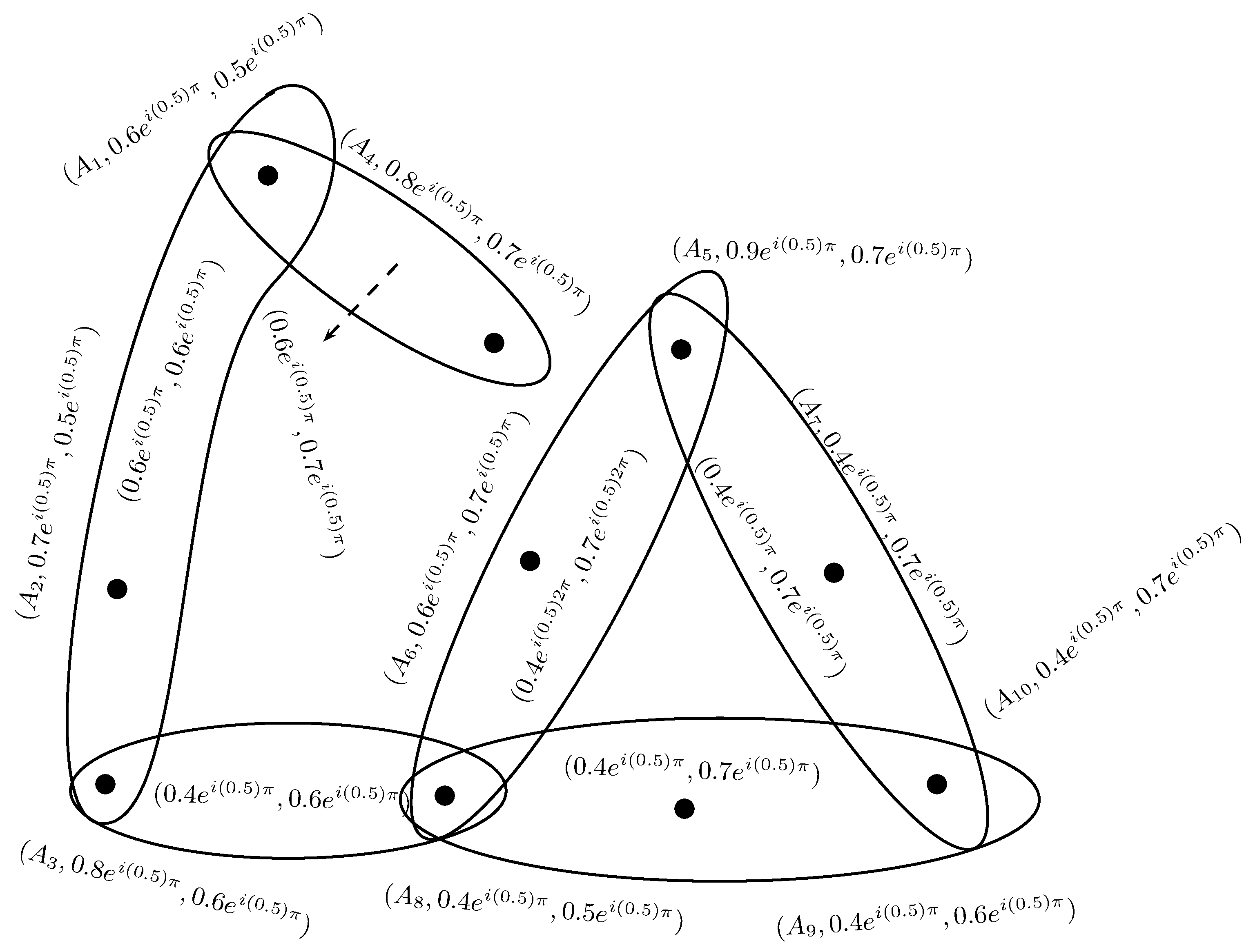
Example 10.
Let be a C6-ROFG on , , , where , , , , , , , and , , , , , , , , are C6-ROFS and C6-ROFR on Y, respectively. The corresponding C6-ROFG is shown in Figure 9.
We now define the more extended concept of complex q-ROF hypergraphs.
Definition 24.
The support of a Cq-ROFS is defined as . The height of a Cq-ROFS is defined as
If , then S is called normal.
Definition 25.
Let Y be a non-trivial set of universe. A complex q-rung orthopair fuzzy hypergraph (Cq-ROFHG) is defined as an ordered pair , where is a finite family of complex q-rung orthopair fuzzy sets on Y and η is a complex q-rung orthopair fuzzy relation on complex q-rung orthopair fuzzy sets ’s such that,
- (i)
- , , for all
- (ii)
- for all
Note that, is the crisp hyperedge of .
Remark 3.
Note that,
- When , C1-ROFHG is a CIFHG.
- When , C2-ROFHG is a CPFHG.
Definition 26.
Let be a Cq-ROFHG. The height of , given as , is defined as , where , , , . Here, and denote the truth and falsity degrees of vertex to hyperedge , respectively.
Definition 27.
Let be a Cq-ROFHG. Suppose that and such that . The level hypergraph of is defined as an ordered pair , where
- (i)
- and ,
- (ii)
- .
Note that, level hypergraph of is a crisp hypergraph.
5. Transversals of Complex q-Rung Orthopair Fuzzy Hypergraphs
In this section we study transversality. Prior to the main definition we need the following auxiliary concept:
Definition 28.
Let be a Cq-ROFHG and for , , , and let be the level hypergraph of . The sequence of complex numbers such that , , , and satisfying the conditions,
- (i)
- if , , , , then , and
- (ii)
- ,
is called the fundamental sequence of , denoted by . The set of level hypergraphs is called the set of core hypergraphs or the core set of , denoted by .
Now we are ready to define:
Definition 29.
Let be a Cq-ROFHG. A complex q-rung orthopair fuzzy transversal (Cq-ROFT) τ is a Cq-ROFs of Y satisfying the condition for all , where is the height of ρ.
A minimal complex q-rung orthopair fuzzy transversal t is the Cq-ROFT of having the property that if , then τ is not a Cq-ROFT of .
Let us denote the family of minimal Cq-ROFTs of by .
Example 12.
Consider a C5-ROFHG on . The C5-ROFR η is given as, , , and . The incidence matrix of is given in Table 2.
The corresponding C5-ROFHG is shown in Figure 12.
By routine calculations, we have , , and . Consider a C5-ROFS of Y such that , , . Note that,
Thus, we have for all Hence, is a C5-ROFT of . Similarly,
are C5-ROFTs of
Definition 30.
A Cq-ROFHG is a partial Cq-ROFHG of if , denoted by . A Cq-ROFHG is ordered if the core set , , ⋯, is ordered, i.e., . is simply ordered if is ordered and
Definition 31.
A Cq-ROFS S on Y is elementary if S is single-valued on . A Cq-ROFHG is elementary if every and η are elementary.
Proposition 1.
If τ is a Cq-ROFT of , then , for all . Furthermore, if τ is minimal Cq-ROFT of , then .
Lemma 1.
Let be a partial Cq-ROFHG of . If is minimal Cq-ROFT of , then there is a minimal Cq-ROFT of such that
Proof.
Let be a Cq-ROFS on Y, which is defined as . Then, is a Cq-ROFT of . Thus, there exists a minimal Cq-ROFT of such that □
Lemma 2.
Let be a Cq-ROFHG then
Proof.
Let and Suppose that for , , , and Define a function by
From definition of , we have . Definition 28 implies that for every , Thus, is a Cq-ROFT of . Since, is minimal Cq-ROFT and for all This implies that is also a Cq-ROFT and but the minimality of implies that . Hence, which implies that for every Cq-ROFT and for each , and so we have □
We now illustrate a recursive procedure to find in Algorithm 1.
| Algorithm 1: To find the family of minimal Cq-ROFTs . |
Let be a Cq-ROFHG having the fundamental sequence , , ⋯, and core set , , ⋯, . The minimal transversal of is determined as follows,
|
Example 13.
Consider a C5-ROFHG on as shown in Figure 13. Let , , , and . Clearly, the sequence satisfies all the conditions of Definition 28. Hence, it is the fundamental sequence of .
Note that, is the minimal transversal of and , is the minimal transversal of , and is the minimal transversal of . Consider
Hence, is a C5-ROFT of .
Lemma 3.
Let be a Cq-ROFHG with . If τ is a Cq-ROFT of , then , for every . If then
Proof.
Since is a Cq-ROFT of , implies that Let , then , , , and . This shows that . If , i.e., is minimal Cq-ROFT then . Thus, we have □
Lemma 4.
Let β be a Cq-ROFT of a Cq-ROFHG . Then, there exists such that .
Proof.
Let . Suppose that is a transversal of and , for such that Let be an elementary Cq-ROFS having support and be an elementary Cq-ROFS having support , for . Then, Algorithm 1 implies that is a Cq-ROFT of and is minimal Cq-ROFT of such that . □
Theorem 3.
Let and be Cq-ROFHGs. Then, is simple, , , for every , and for every Cq-ROFS , exactly one of the conditions must satisfy,
- (i)
- , for some or
- (ii)
- there is and , where , , such that , i.e., ξ is not a Cq-ROFT of .
Proof.
Let . Since, the family of all minimal Cq-ROFTs form a simple Cq-ROFHG on . Lemma 3 implies that every edge of has height . Let be an arbitrary Cq-ROFS.
- Case(i)
- If is a Cq-ROFT of , then Lemma 4 implies the existence of a minimal Cq-ROFT such that . Thus, the condition (i) holds and (ii) violates.
- Case(ii)
- If is not a Cq-ROFT of , then there is an edge such that . If condition (i) holds, implies that , which is the contradiction against the fact that is Cq-ROFT. Hence, condition (i) does not hold and (ii) is satisfied.
Conversely, suppose that satisfies all properties as mentioned above and . Let , then we obtain and conditions (ii) is not satisfied, so is Cq-ROFT of . If t is minimal Cq-ROFT of and , t does not satisfy (ii), this implies the existence of such that , hence . Since, t is minimal Cq-ROF which implies that , and t were chosen arbitrarily therefore, we have . □
The construction of fundamental subsequence and subcore of Cq-ROFHG is discussed in Algorithm 2.
| Algorithm 2: Construction of fundamental subsequence and subcore. |
| Let be a Cq-ROFHG and be a partial Cq-ROFHG of . The fundamental subsequence is constructed as follows: Let and .
|
Definition 32.
Let be a Cq-ROFHG having fundamental subsequence and subcore of . The Cq-ROFT core of is defined as an elementary Cq-ROFHG such that,
- (i)
- , i.e., is also a fundamental subsequence of ,
- (ii)
- height of every is iff is an hyperedge of .
Theorem 4.
For every Cq-ROFHG, we have .
Proof.
Let and . Definition 32 implies that and is an hyperedge of . Since and is a transversal of therefore Thus, is a Cq-ROFT of .
Let and . Definition 28 implies that , for . Definition of subcore implies the existence of an hyperedge
of such that and . For , we have . Hence, is a Cq-ROFT of .
Let is a Cq-ROFT of . This implies that there is such that . But is a Cq-ROFT of and implies that . Thus, . Also implies that . □
Although can be taken as a minimal transversal of , it is not necessary for to be the minimal transversal of , for all , and . Furthermore, it is not necessary for the family of minimal Cq-ROFTs to form a hypergraph on Y. For those Cq-ROFTs that satisfy the above property, we have:
Definition 33.
A Cq-ROFT τ having the property that , for all , and is called the locally minimal Cq-ROFT of . The collection of all locally minimal Cq-ROFTs of is represented by .
Note that, , but the converse is not generally true.
Example 14.
Theorem 5.
Let be an ordered Cq-ROFHG with . If is a minimal transversal of , then there exists such that and is a minimal transversal of , for all . In particular, if , then there exists a locally minimal Cq-ROFT and
Proof.
Let . Since, is an ordered Cq-ROFHG, therefore . Also, there exists such that . Following this iterative procedure, we have a nested sequence of minimal transversals, where every . Let be an elementary Cq-ROFS having height and support . Let us define such that , that generates the required minimal Cq-ROFT of . If , is locally minimal Cq-ROFT of . Hence, □
Theorem 6.
Let be a simply ordered Cq-ROFHG with . If , then there exists such that .
Proof.
Let and is a simply ordered Cq-ROFHG. Theorem 5 implies that a nested sequence of minimal transversals can be constructed. Let Let be an elementary Cq-ROFS having height and support such that generates the locally minimal Cq-ROFT of with . □
6. Application
Most of the previous studies use crisp hypergraphs to analyze the co-authorship relation between two or more authors as a collaboration. In this section, we consider a Cq-ROFHG model of co-authorship network to represent the collaboration relations between authors having uncertainty and vagueness of periodic nature simultaneously. The next comparison law between Cq-ROFNs will be helpful in our application:
Definition 34.
Let be a Cq-ROFN. Then, the score function of is defined as,
The accuracy of is defined as,
For two Cq-ROFNs and ,
- 1.
- if , then ,
- 2.
- if , then
- if , then ,
- if , then .
6.1. A C6-ROFHG Model of Research Collaboration Network
A collaboration network is a group of independent organizations or people that interact to complete a particular goal for achieving better collective results by means of the joint execution of a task. The entities of a collaborative network may be geographically distributed and heterogeneous in terms of their culture, goals, and operating environment but they collaborate to achieve compatible or common goals. For decades, science academies have been interested in research collaboration. The most common reasons for research collaboration are funding, more experts working on the same project imply the more chances for effectiveness, productivity, and innovativeness. Nowadays, most of the public research is based on the collaboration of different types of expertise from different disciples and different economic sectors. In this section, we study a research collaboration network model through C6-ROFHG. Consider a science academy that wants to select an author among a group of researchers that has the best collaborative skills. For this purpose, the following characteristics can be considered:
- Cooperative spirit
- Mutual respect
- Critical thinking
- Innovations
- Creativity
- Embrace diversity
We construct a C6-ROFHG on . The universe Y represents the group of authors as the vertices of and these authors are grouped through hyperedges if they have worked together on some projects. The truth-membership of each author represents the collaboration strength and falsity-membership describes the opposite behavior of the corresponding author. Suppose that a team of experts assigns that the collaboration power of is and non-collaborative behavior is after carefully observing the different attributes. The corresponding phase terms illustrate the specific period of time in which the collaborative behavior of an author varies. We model this data as . The C6-ROFHG model of collaboration network is shown in Figure 15.
The membership degrees of hyperedges represent the collective degrees of collaboration and non-collaboration of the corresponding authors combined through an hyperedge. The adjacency matrix of this network is given in Table 3, Table 4 and Table 5.
The score values and choice values of a C6-ROFHG are calculated as follows,
respectively. These values are given in Table 6.
The choice values of Table 6 show that is the author having maximum strength of collaboration and good collective skills among all the authors. Similarly, the choice values of all authors represent the strength of their respective collaboration skills in a specific period of time. The method adopted in our model to select the author having best collaboration skills is given in Algorithm 3.
| Algorithm 3: Selection of author having maximum collaboration skills. |
|
6.2. Comparative Analysis
The proposed Cq-ROF model is more flexible and compatible to the system when the given data ranges over complex subset with unit disk instead of real subset with We illustrate the flexibility of our proposed model by taking an example. Consider an educational institute that wants to establish its minimum branches in a particular city in order to facilitate the maximum number of students according to some parameters such as transportation, suitable place, connectivity with the main branch, and expenditures. Suppose a team of three decision-makers selects the different places. Let be the set of places where the team is interested to establish the new branches. After carefully observing the different attributes, the first decision-makers assign the membership and non-membership degrees to support the place as and , respectively. The phase terms represent the period of time for which the place can attract maximum number of students. This information is modeled using a CIFS as . Note that, and Similarly, he models the other places as, , . We denote this CIF model as
All CIF grades are CPF as well as Cq-ROF grades. We find the score functions of the above values using the formulas , , and . The results corresponding to these three approaches are given in Table 7.
Suppose that the second decision-maker assigns the membership values to these places as, . This information can not be modeled using CIFS as . We model this information using a CPFS and the corresponding model is given as,
All CPF grades are also Cq-ROF grades. We find the score functions of the above values using the formulas and . The results corresponding to these two approaches are given in Table 8.
We now suppose that the third decision-maker assigns the membership values to these places as, . This information can not be modeled using CIFS and CPFS as , . We model this information using a C3-ROFS and the corresponding model is given as,
We find the score functions of the above values using the formula . The score values of C3-ROF information are given as,
Note that is the best optimal choice to establish a new branch according to the given parameters. We see that every CIF grade is a CPF grade, as well as a Cq-ROF grade, however there are Cq-ROF grades that are not CIF nor CPF grades. This implies the generalization of Cq-ROF values. Thus the proposed Cq-ROF model provides more flexibility due to its most prominent feature that is the adjustment of the range of demonstration of given information by changing the value of parameter q, . The generalization of our proposed model can also be observed from the reduction of Cq-ROF model to CIF and CPF models for and , respectively.
7. Conclusions and Future Directions
Fuzzy sets and intuitionistic fuzzy sets cannot handle imprecise, inconsistent, and incomplete information of periodic nature. They lack the capability to model two-dimensional phenomena. To vercome this difficulty, the concept of complex fuzzy sets was introduced by Ramot et al. [2]. Their phase term is the critical feature of the complex fuzzy set model. The potential of a complex fuzzy set for representing two-dimensional phenomena makes it superior when it comes to handle ambiguous and intuitive information, especially in time-periodic phenomena.
A Cq-ROF model is a generalized form of both the complex intuitionistic fuzzy and complex Pythagorean fuzzy models. Indeed, a Cq-ROF model reduces to a CIF model when , and it becomes a CPF model when . The Cq-ROF model provides a sufficiently wide space of permissible complex orthopairs.
Hypergraphs are mathematical tools for the representation and understanding of problems in a wide variety of scientific fields. In this article, we have applied the most fruitful concept of Cq-ROFSs to hypergraphs. We have defined the novel concepts of Cq-ROFSs, Cq-ROFGs, Cq-ROFHGs, level hypergraphs, and Cq-ROF transversals of Cq-ROFHGs. Further, we have proved that a C1-ROFHG is a CIFHG and a C2-ROFHG is a CPFHG. We have also designed algorithms to construct minimal transversals, fundamental subsequence and subcore of a Cq-ROFHG. Finally, we have illustrated a real-life application of Cq-ROFHGs in collaboration networks that enhances the motivation of this research article.
We aim to broaden our study in the future with the analysis of (1) Complex fuzzy directed hypergraphs, (2) Complex bipolar neutrosophic hypergraphs, (3) Fuzzy rough soft directed hypergraphs and (4) Fuzzy rough neutrosophic hypergraphs.
Author Contributions
investigation, A.L., M.A., A.N.A.-K. and J.C.R.A.; writing—original draft, A.L. and M.A.; writing—review and editing, A.N.A.-K. and J.C.R.A.
Funding
This research received no external funding.
Acknowledgments
This project was funded by the Deanship of Scientific Research (DSR), King Abdulaziz University, Jeddah, under grant No. (DF-121-130-1441). The authors, therefore, gratefully acknowledge DSR technical and financial support
Conflicts of Interest
The authors declare no conflict of interest.
References
- Zadeh, L.A. Fuzzy sets. Inf. Control 1965, 8, 338–353. [Google Scholar] [CrossRef] [Green Version]
- Ramot, D.; Milo, R.; Friedman, M.; Kandel, A. Complex fuzzy sets. IEEE Trans. Fuzzy Syst. 2002, 10, 171186. [Google Scholar] [CrossRef]
- Yazdanbakhsh, O.; Dick, S. A systematic review of complex fuzzy sets and logic. Fuzzy Sets. Syst. 2018, 338, 1–22. [Google Scholar] [CrossRef]
- Atanassov, K.T. Intuitionistic fuzzy sets. Fuzzy Sets Syst. 1983, 20, 87–96. [Google Scholar] [CrossRef]
- Liu, X.; Kim, H.; Feng, F.; Alcantud, J.C.R. Centroid transformations of intuitionistic fuzzy values based on aggregation operators. Mathematics 2018, 6, 215. [Google Scholar] [CrossRef]
- Feng, F.; Fujita, H.; Ali, M.I.; Yager, R.R.; Liu, X. Another view on generalized intuitionistic fuzzy soft sets and related multiattribute decision making methods. IEEE Trans. Fuzzy Syst. 2019, 27, 474–488. [Google Scholar] [CrossRef]
- Shumaiza; Akram, M.; Al-Kenani, A.N.; Alcantud, J.C.R. Group decision-making based on the VIKOR method with trapezoidal bipolar fuzzy information. Symmetry 2019, 11, 1313. [Google Scholar] [CrossRef]
- Akram, M.; Arshad, M. A novel trapezoidal bipolar fuzzy TOPSIS method for group decision-making. Group Decis. Negot. 2019, 28, 565–584. [Google Scholar] [CrossRef]
- Alcantud, J.C.R.; Biondo, A.; Giarlotta, A. Fuzzy politics I: The genesis of parties. Fuzzy Sets Syst. 2018, 349, 71–98. [Google Scholar] [CrossRef]
- Alcantud, J.C.R.; Giarlotta, A. Necessary and possible hesitant fuzzy sets: A novel model for group decision-making. Inf. Fusion 2019, 46, 63–76. [Google Scholar] [CrossRef]
- Yager, R.R.; Abbasov, A.M. Pythagorean membership grades, complex numbers and dcision making. Int. J. Intell. Syst. 2013, 28, 436–452. [Google Scholar] [CrossRef]
- Yager, R.R. Pythagorean membership grades in multi-criteria decision making. IEEE Trans. Fuzzy Syst. 2014, 22, 958–965. [Google Scholar] [CrossRef]
- Yager, R.R. Generalized orthopair fuzzy sets. IEEE Trans. Fuzzy Syst. 2017, 25, 1222–1230. [Google Scholar] [CrossRef]
- Liu, P.D.; Wang, P. Some q-rung orthopair fuzzy aggregation operators and their applications to multi-attribute decision making. Int. J. Intell. Syst. 2018, 33, 259–280. [Google Scholar] [CrossRef]
- Alcantud, J.C.R.; Muñoz Torrecillas, M.J. Intertemporal choice of fuzzy soft sets. Symmetry 2018, 10, 371. [Google Scholar] [CrossRef]
- Alcantud, J.C.R.; García-Sanz, M.D. Evaluations of infinite utility streams: Pareto efficient and egalitarian axiomatics. Metroeconomica 2013, 64, 432–447. [Google Scholar] [CrossRef]
- Alcantud, J.C.R.; García-Sanz, M.D. Paretian evaluation of infinite utility streams: An egalitarian criterion. Econ. Lett. 2010, 106, 209–211. [Google Scholar] [CrossRef] [Green Version]
- Wei, G.; Gao, H.; Wei, Y. Some q-rung orthopair fuzzy heronian mean operators in multiple attribute decision making. Int. J. Intell. Syst. 2018, 33, 1426–1458. [Google Scholar] [CrossRef]
- Bai, K.; Zhu, X.; Wang, J.; Zhang, R. Some partitioned maclaurin symmetric mean based on q-rung orthopair fuzzy information for dealing with multi-attribute group decision making. Symmetry 2018, 10, 383. [Google Scholar] [CrossRef]
- Li, L.; Zhang, R.; Wang, J.; Shang, X.; Bai, K. A novel approach to multi-attribute group decision-making with q-rung picture linguistic information. Symmetry 2018, 10, 172. [Google Scholar] [CrossRef]
- Alkouri, A.; Salleh, A. Complex intuitionistic fuzzy sets. AIP Conf. Proc. 2012, 14, 464–470. [Google Scholar]
- Ullah, K.; Mahmood, T.; Ali, Z.; Jan, N. On some distance measures of complex Pythagorean fuzzy sets and their applications in pattern recognition. Complex Intell. Syst. 2019. forthcoming. [Google Scholar] [CrossRef]
- Rosenfeld, A. Fuzzy graphs. In Fuzzy Sets and Their Applications; Zadeh, L.A., Fu, K.S., Shimura, M., Eds.; Academic Press: New York, NY, USA, 1975; pp. 77–95. [Google Scholar]
- Bhattacharya, P. Some remarks on fuzzy graphs. Pattern Recognit. Lett. 1987, 6, 297–302. [Google Scholar] [CrossRef]
- Thirunavukarasu, P.; Suresh, R.; Viswanathan, K.K. Energy of a complex fuzzy graph. Int. J. Math. Sci. Eng. Appl. 2016, 10, 243–248. [Google Scholar]
- Parvathi, R.; Karunambigai, M.G. Intuitionistic fuzzy graphs. In Computational Intelligence, Theory and Applications; Reusch, B., Ed.; Springer: Berlin/Heidelberg, Germany, 2006. [Google Scholar]
- Akram, M.; Naz, S. Energy of Pythagorean fuzzy graphs with applications. Mathematics 2018, 6, 136. [Google Scholar] [CrossRef]
- Akram, M.; Habib, A. q-Rung orthopair fuzzy competition graphs with application in the soil ecosystem. Mathematics 2018, 7, 91. [Google Scholar]
- Akram, M.; Habib, A.; Koam, A.N. A novel description on edge-regular q-rung picture fuzzy graphs with application. Symmetry 2019, 11, 489. [Google Scholar] [CrossRef]
- Yaqoob, N.; Gulistan, M.; Kadry, S.; Wahab, H. Complex intuitionistic fuzzy graphs with application in cellular network provider companies. Mathematics 2019, 7, 35. [Google Scholar] [CrossRef]
- Yaqoob, N.; Akram, M. Complex neutrosophic graphs. Bull. Comput. Appl. Math. 2018, 6, 85–109. [Google Scholar]
- Akram, M.; Naz, S. A novel decision-making approach under complex Pythagorean fuzzy environment. Math. Comput. Appl. 2019, 24, 73. [Google Scholar] [CrossRef]
- Berge, C. Graphs and Hypergraphs; North-Holland Publishing Company: Amsterdam, The Netherlands, 1973. [Google Scholar]
- Boulet, R.; Fla´via Barros-Platiau, A.; Mazzega, P. Environmental and Trade Regimes: Comparison of Hypergraphs Modeling the Ratifications of UN Multilateral Treaties. In Law, Public Policies and Complex Systems; Boulet, R., Lajaunie, C., Mazzega, P., Eds.; Springer: Berlin/Heidelberg, Germany, 2019; Chapter 11. [Google Scholar]
- Strzelecka, A.; Skworcow, P. Modelling and simulation of utility service provision for sustainable communities. Int. J. Elect. Tel. 2012, 58, 389–396. [Google Scholar] [CrossRef]
- Han, Y.; Zhou, B.; Pei, J.; Jia, Y. Understanding importance of collaborations in co-authorship networks: A supportiveness analysis approach. In Proceedings of the 2009 SIAM International Conference on Data Mining, Sparks, NV, USA, 30 April–2 May 2009; pp. 1112–1123. [Google Scholar]
- Zhang, Z.K.; Liu, C. A hypergraph model of social tagging networks. J. Stat. Mech. Theory Exp. 2010, 10, 10005. [Google Scholar] [CrossRef]
- Ouvrard, X.; Goff, J.M.L.; Marchand-Maillet, S. Networks of collaborations: Hypergraph modeling and visualisation. arXiv 2017, arXiv:1707.00115. [Google Scholar]
- Kaufmann, A. Introduction a la Theorie des Sous-Ensemble Flous 1; Masson: Paris, France, 1977. [Google Scholar]
- Lee-kwang, H.; Lee, K.-M. Fuzzy hypergraph and fuzzy partition. IEEE Trans. Syst. Man Cybern. 1995, 25, 196–201. [Google Scholar] [CrossRef]
- Mordeson, J.N.; Nair, P.S. Fuzzy Graphs and Fuzzy Hypergraphs, 2nd ed.; Physica Verlag: Heidelberg, Germany, 1998. [Google Scholar]
- Goetschel, R.H.; Craine, W.L.; Voxman, W. Fuzzy transversals of fuzzy hypergraphs. Fuzzy Sets. Syst. 1996, 84, 235–254. [Google Scholar] [CrossRef]
- Parvathi, R.; Thilagavathi, S.; Karunambigai, M.G. Intuitionistic fuzzy hypergraphs. Cyber. Inf. Tech. 2009, 9, 46–53. [Google Scholar]
- Akram, M.; Dudek, W.A. Intuitionistic fuzzy hypergraphs with applications. Inf. Sci. 2013, 218, 182–193. [Google Scholar] [CrossRef]
- Parvathi, R.; Akram, M.; Thilagavathi, S. Intuitionistic fuzzy shortest hyperpath in a network. Inf. Process. Lett. 2013, 113, 599–603. [Google Scholar]
- Akram, M.; Luqman, A. Bipolar neutrosophic hypergraphs with applications. J. Intell. Fuzzy Syst. 2017, 33, 1699–1713. [Google Scholar] [CrossRef]
- Akram, M.; Sarwar, M. Transversals of m-polar fuzzy hypergraphs with applications. J. Intell. Fuzzy Syst. 2017, 33, 351–364. [Google Scholar] [CrossRef]
- Luqman, A.; Akram, M.; Al-Kenani, A.N. q-Rung orthopair fuzzy hypergraphs with applications. Mathematics 2019, 7, 260. [Google Scholar] [CrossRef]
- Luqman, A.; Akram, M.; Koam, A.N. An m-polar fuzzy hypergraph model of granular computing. Symmetry 2019, 11, 483. [Google Scholar] [CrossRef]
- Luqman, A.; Akram, M.; Koam, A.N. Granulation of hypernetwork models under the q-rung picture fuzzy environment. Mathematics 2019, 7, 496. [Google Scholar] [CrossRef]
Figure 1.
Complex intuitionistic fuzzy hypergraph.

Figure 2.
level hypergraph of H.

Figure 3.
Complex intuitionistic fuzzy line graph of H.

Figure 4.
Two-section of complex intuitionistic fuzzy hypergraph.

Figure 5.
Complex Pythagorean fuzzy hypergraph.

Figure 6.
level hypergraph of .

Figure 7.
Line graph of complex Pythagorean fuzzy hypergraph .

Figure 8.
Two-section of complex Pythagorean fuzzy hypergraph .

Figure 9.
Complex six-rung orthopair fuzzy graph.

Figure 10.
Complex six-rung orthopair fuzzy hypergraph.

Figure 11.
The level hypergraph of .

Figure 12.
Complex five-rung orthopair fuzzy hypergraph.

Figure 13.
Complex five-rung orthopair fuzzy hypergraph.

Figure 14.
Complex six-rung orthopair fuzzy hypergraph.

Figure 15.
Complex six-rung orthopair fuzzy hypergraph model of collaboration network.


Table 1.
Incidence matrix of C6-ROFHG .
Table 2.
Incidence matrix of C5-ROFHG .
Table 3.
Adjacency matrix of collaboration network.
Table 4.
Adjacency matrix of collaboration network.
Table 5.
Adjacency matrix of collaboration network.
Table 6.
Score and choice values.
| 0 | 0 | 0 | 0 | 0 | 0 | 0 | |||||
| 0 | 0 | 0 | 0 | 0 | 0 | 0 | 0 | ||||
| 0 | 0 | 0 | 0 | 0 | 0 | 0 | |||||
| 0 | 0 | 0 | 0 | 0 | 0 | 0 | 0 | 0 | |||
| 0 | 0 | 0 | 0 | 0 | 0 | ||||||
| 0 | 0 | 0 | 0 | 0 | 0 | 0 | 0 | ||||
| 0 | 0 | 0 | 0 | 0 | 0 | 0 | 0 | ||||
| 0 | 0 | 0 | 0 | 0 | |||||||
| 0 | 0 | 0 | 0 | 0 | 0 | 0 | 0 | ||||
| 0 | 0 | 0 | 0 | 0 | 0 |
Table 7.
Comparative analysis of CIF, CPF, and C3-ROF models.
| Methods | Score Values | Ranking |
|---|---|---|
| CIF model | 0.4 1.0 0.6 | |
| CPF model | 0.4 0.9 0.42 | |
| C3-ROF model | 0.104 0.67 0.234 |
Table 8.
Comparative analysis of CPF, and C3-ROF models.
| Methods | Score Values | Ranking |
|---|---|---|
| CPF model | 0.4 0.9 0.48 | |
| C3-ROF model | 0.104 0.67 0.436 |
© 2019 by the authors. Licensee MDPI, Basel, Switzerland. This article is an open access article distributed under the terms and conditions of the Creative Commons Attribution (CC BY) license (http://creativecommons.org/licenses/by/4.0/).
Share and Cite
MDPI and ACS Style
Luqman, A.; Akram, M.; Al-Kenani, A.N.; Alcantud, J.C.R. A Study on Hypergraph Representations of Complex Fuzzy Information. Symmetry 2019, 11, 1381. https://0-doi-org.brum.beds.ac.uk/10.3390/sym11111381
AMA Style
Luqman A, Akram M, Al-Kenani AN, Alcantud JCR. A Study on Hypergraph Representations of Complex Fuzzy Information. Symmetry. 2019; 11(11):1381. https://0-doi-org.brum.beds.ac.uk/10.3390/sym11111381
Chicago/Turabian StyleLuqman, Anam, Muhammad Akram, Ahmad N. Al-Kenani, and José Carlos R. Alcantud. 2019. "A Study on Hypergraph Representations of Complex Fuzzy Information" Symmetry 11, no. 11: 1381. https://0-doi-org.brum.beds.ac.uk/10.3390/sym11111381
Note that from the first issue of 2016, this journal uses article numbers instead of page numbers. See further details here.