Quasi-Periodic Oscillating Flows in a Channel with a Suddenly Expanded Section


Department of Aeronautics and Astronautics, Tokyo Metropolitan University, Hino 191-0065, Japan
*
Author to whom correspondence should be addressed.
Symmetry 2019, 11(11), 1403; https://0-doi-org.brum.beds.ac.uk/10.3390/sym11111403
Submission received: 15 October 2019
/
Revised: 7 November 2019
/
Accepted: 10 November 2019
/
Published: 13 November 2019
(This article belongs to the Special Issue Symmetry in Fluid Flow)
Abstract
:In this study, two-dimensional numerical simulation was carried out for an oscillatory flow between parallel flat plates having a suddenly expanded section. Governing equations were discretized with the second-order accuracy by a finite volume method on an unequal interval mesh system resolving finer near walls and corners to obtain the characteristics of the oscillatory flow accurately. Amplitude spectrums of a velocity component were obtained to investigate the periodic characteristics of the oscillatory flow. At low Reynolds numbers, the flow is periodic because the spectrum mostly consists of harmonic components, and then at high Reynolds numbers, it transits to a quasi-periodic flow mixed with non-harmonic components. In conjunction with the periodic oscillation of a main flow, separation vortices that are not uniform in size are generated from the corner of a sudden contraction part and pass through a downstream region coming into contact with the wall. The number of the vortices decreases rapidly after they are generated, but the vortices are generated again in the downstream region. In order to specify where aperiodicity is generated, the turbulent kinetic energy is introduced, and it is decomposed into the harmonic and non-harmonic components. The peaks of the non-harmonic component are generated in the region of the expanded section.

1. Introduction
Fluid mechanics concern gas and liquid in motion. In general, as the crucial parameter known as the Reynolds number increases, the flow tends to be more complicated because of the characteristic of non-linearity peculiar to fluids. The state of fluid motion can be classified into laminar flow, transition, or turbulent flow. In various industrial applications related to fluid motion as well as the natural phenomena such as atmospheric and oceanic flows, the identification and the control of fluid flow are of great importance. The fluid flow sometimes exhibits the transitional behavior between the laminar and turbulent regimes at a certain range of Reynolds numbers. The transitional flow is considered to be related to the instability of the base laminar flow. However, the complex mechanism of such flow transition, where the flow characteristic changes from a simple state to another more complicated state, has not been sufficiently understood yet. Herein, the three key words are recalled as follows:
- Stability: When a small disturbance is added to a steady flow, if any disturbance is attenuated, the flow is “stable”. Conversely, if one of any disturbance grows, its state is “unstable”.
- Turbulence: In this paper, irregularly changing flow is treated as “turbulent flow”, but the definition of the turbulent flow has not always been obvious. Here is a summary of the characteristics of turbulent flow. The physical quantities such as velocity and static pressure fluctuate irregularly in time and space, and the transport and exchange are much faster than the molecular transport. The energy of fluctuation is transferred from usual large-scaled vortices to small-scaled ones.
- Transition: A process in which the flow changes from a stable state to an unstable state as the Reynolds number increases is called a “transition”. The forms of transition process differ depending on the type of the base flow. In the case of a plane Poiseuille flow, the oscillatory flow is quasi-periodic just above the critical Reynolds number.
It is well known that the plane Poiseuille flow, which is driven by a constant pressure gradient between the parallel flat plates, has a steady exact solution of velocity profile. However, this solution is not always realized for such a condition in which the two-dimensional disturbance called the Tollmien–Schlichting (T-S) wave grows. It is known that the minimal value of the critical Reynolds number for the plane Poiseuille flow is about 2900 for non-linear disturbance [1]. In a region over the critical value, numerical simulations have revealed that an aperiodic oscillatory flow accompanying the stimulation, such as a modulated wave or chaos, takes place depending on a combination of the Reynolds number and wavenumber [2].
In a channel of parallel flat plates with suddenly expanded sections of a rectangle, a transition from a steady flow to a periodic oscillating flow occurs at a lower Reynolds number than that of the plane Poiseuille flow. This periodic oscillation is attributed to the Kelvin–Helmholtz instability [3]. This critical Reynolds number depends on the size [4] and the number [5] of the suddenly expanded sections, the symmetry for the center line of the channel [6], the boundary condition in the mainstream direction, and so on. Concerning the boundary condition in the mainstream direction, either a periodic boundary condition [7] or an inlet–outlet boundary condition [8] in which a fluid is not recirculated is given. It is known that the critical Reynolds number in the inlet–outlet boundary condition is higher than that in the periodic boundary condition. Although the flow exhibits periodic oscillation just above the critical Reynolds number, it may transit to an aperiodic oscillatory flow as observed in the plane Poiseuille flow if the Reynolds number becomes higher.
For the channel flow having such a suddenly expanded section, researchers have tried to excite instability by forced pulsating flow [9], by a non-uniform thermal field [10], or by both of them [11,12]. Thereby, a quasi-periodic oscillatory flow with a modulated wave or irregularity appears, and finally it reaches a turbulent state in which the fundamental frequency cannot be recognized. The aperiodic oscillatory flow may occur under these unstable conditions even if the self-sustaining oscillating flow is periodic under the uniform temperature condition. In these studies, the channels that expanded suddenly on only one side were used. The periodic boundary condition was imposed in the mainstream direction in the two-dimensional computations, whereas the channels with multiple suddenly expanded sections were used in the experiments. A similar transition pattern was observed in a channel with suddenly expanded sections, which was symmetric with respect to the center line of the channel [13].
In facilities such as industrial machinery and environmental equipment, there are many flow channels with sudden-expanded sections. By providing a sudden-expanded part, the mixing of heat and mass in the working fluid can be promoted. The flow considered here is a two-dimensional flow through a symmetric channel with a sudden expanded section, which is considered to be the simplest model for an actual facility. In general, pipes and plates are installed in the expanded part, where pressure, temperature, and humidity are adjusted and exhaust gases, dusts and impurities are removed [14]. Especially for automotive equipment, technology development has been continued to improve energy efficiency. For example, in a honeycomb monolith reactor [15] and wall flow ceramic filters [16], which are widely utilized in automotive exhaust gas after treatment systems, improvements were reported. Interestingly, as a case in which working fluids other than the continuum were used, numerical simulations of dilute flows in microchannels using the lattice Boltzmann method [17] were performed.
On the other hand, the flow between parallel plates with only a sudden reduction part is classified as a separation flow. The flow of steady state becomes irregular immediately after passing through the sudden reduction part, and the vortices are generated irregularly behind the separation region. In a channel flow with a partially expanded part, the inlet/outlet boundary conditions may cause not only oscillatory characteristics as observed in the plane Poiseuille flow but also irregular characteristics peculiar to separation flow. Moreover, they can affect each other. In this study, we verify these possibilities.
Nowadays, computational fluid dynamics (CFD) can treat quite large Reynold number flows using powerful computers where the Navier–Stokes equation is numerically solved. For analyzing a turbulent flow, turbulent models such as Reynolds-averaged Navier–Stokes (RANS) or large-eddy simulation (LES) are usually used, but meanwhile, it has been attempted to analyze turbulent channel flows with direct numerical simulation (DNS) [18], in which the Navier–Stokes equation is directly solved with a high-resolved mesh system without using any turbulent models.
In this study, we focused on a channel flow with a suddenly expanded section being symmetric with respect to the center line of the channel and carried out two-dimensional numerical simulation for a process in which a periodic oscillating flow becomes aperiodic as the Reynolds number increases. The oscillatory characteristic in the inlet–outlet boundary condition can be observed more easily than that in the periodic boundary condition, because disturbance does not circulate in the channel. As mention above, in the inlet–outlet boundary condition, aperiodic flow is expected to occur at higher Reynolds numbers than in the periodic boundary condition. However, this condition requires quite a large-scale and high-resolved mesh, i.e., high computational resources. Therefore, no computations of such an inlet–outlet boundary condition have been reported.
The shape of the suddenly expanded section that the present study considers is that the expansion ratio is 3 and the aspect ratio is 7/3 (its definition is shown later). The critical Reynolds number Rec in this aspect ratio and boundary condition was reported as Rec = 843 [8] or 1000 < Rec < 1100 [19]. Therefore, in this study, the computations were carried out for the range of Reynolds numbers 1200 ≤ Re ≤ 2000, where the flow should exhibit oscillatory flow, keeping a certain numerical accuracy.
2. Methods
2.1. Geometry of a Channel and Governing Equations
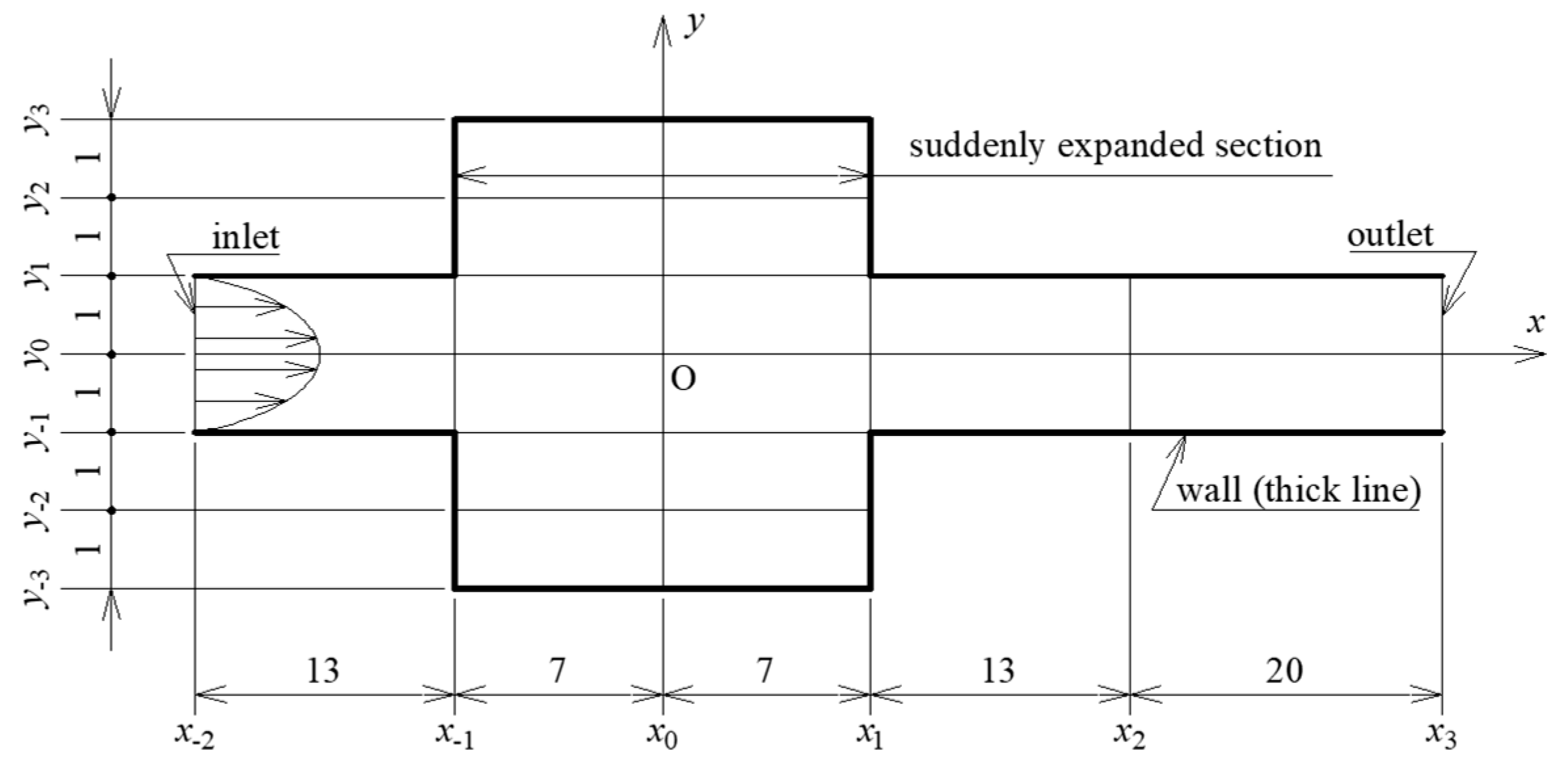
Figure 1 shows a channel geometry where thick lines correspond to wall surfaces. A fluid flows from left to right between the two parallel flat plates. This geometry is set in two-dimensional space, where the coordinate origin O is set at the center of the suddenly expanded section, the x-coordinate is taken along the parallel flat plates, and the y-coordinate is perpendicular to the x-coordinate. In order to describe the channel structure accurately, serial numbers are assigned to the coordinates of the key points of the channel based on the origin O (x0, y0). Each length of the sides is shown in Figure 1. Parameters describing the shape of the channel are the expansion ratio Ex = (y3 − y−3)/(y1 − y−1) = 3 and the aspect ratio As = (x1 − x−1)/(y3 − y−3) = 7/3.
Supposing an incompressible Newtonian fluid, pressure p and velocity u = (u, v) are numerically obtained as a function of time t and x = (x, y). Dimensionless governing equations are the Equation of continuity (1) and the Navier–Stokes Equation (2). In this study, viscous dissipation is ignored, and therefore, the energy equation is not taken into account.
The Reynolds number is defined as Re = U*δ*/ν*. On the inlet, the characteristic velocity U* [m/s] is taken as the maximum value of the velocity component u* obtained from the exact solution of the plane Poiseuille flow, and the characteristic length δ* [m] is the half height of the parallel flat plates. Coefficients of kinetic viscosity ν* [m2/s] and density ρ* [kg/m3] are assumed to be constant. Representing dimension values with the star (*), the physical values are made dimensionless as t = t*U*/δ*, x = x*/δ*, p = p*/ρ*U*2, and u = u*/U*.
2.2. Numerical Solutions
OpenFOAM 2.3.1 [20] was employed as a simulation tool. Some examples using this tool for unsteady laminar flows in a channel whose cross-sectional area changes suddenly are the flow through a sudden expansion part in a circular pipe [21] and that in a rectangular duct [22,23].
The governing Equations (1) and (2) were discretized by a finite volume method. To be based on them, the pressure p and the velocity u were calculated by the PISO (Pressure Implicit with Splitting of Operators) algorithm. The numerical schemes were constructed with the second-order accuracy in all, where the second-order accurate Crank–Nicholson scheme for the time t and the second-order accurate central-difference scheme for the space x were used. The pressure p and the velocity u are solved by the GAMG (geometric–algebraic multi-grid) method and Gauss–Seidel method, respectively. The iterative calculation was performed until the residual value, which was defined by normalizing the L1 norm of the residual vector [24] until it became less than 10−10.
The boundary conditions are as follows. For an inlet boundary condition, the velocity u is given by the parabolic distribution as the exact solution of the plane Poiseuille flow, and the pressure p is the zero gradient in the streamwise direction, as shown in Equation (3).
To cope with an outlet boundary condition for u, the Sommerfeld radiation condition is used, and p is set so that the mean on the outlet is zero, as shown in Equation (4). Equation (4) is the advection equation about u. It means that the velocity upstream by UcΔt in the x direction from the boundary surface at a current time step is applied to the velocity on the boundary surface at the next time step, where Δt is the time step. For the advection velocity Uc of the Sommerfeld radiation condition, the area-averaged velocity is applied at each boundary surface subdivided by a mesh.
On the walls, the no-slip condition is applied for u, and the zero gradient in the normal direction is used for p, as shown in Equation (5).
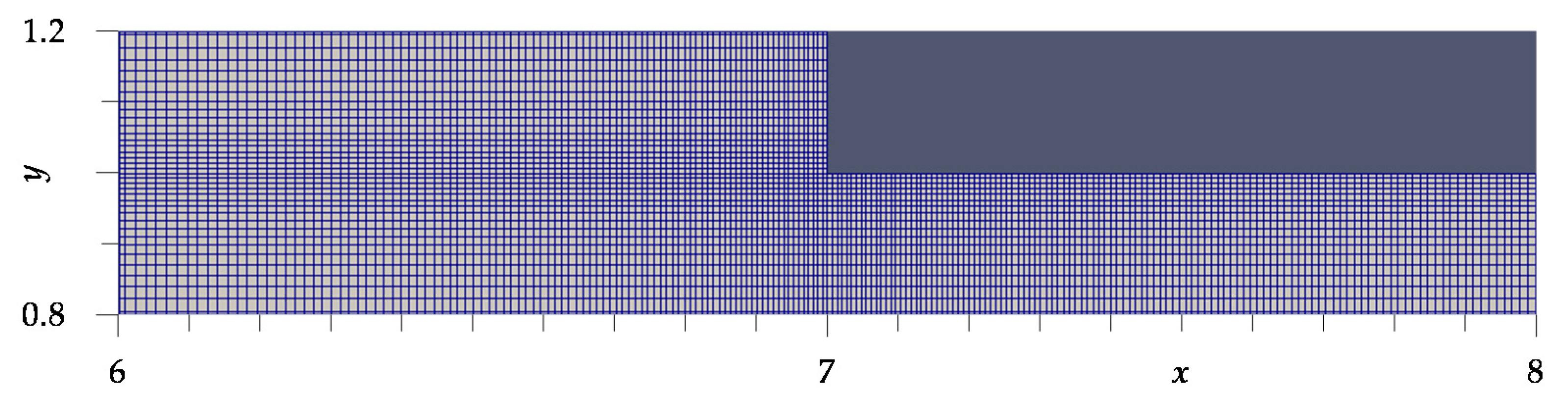
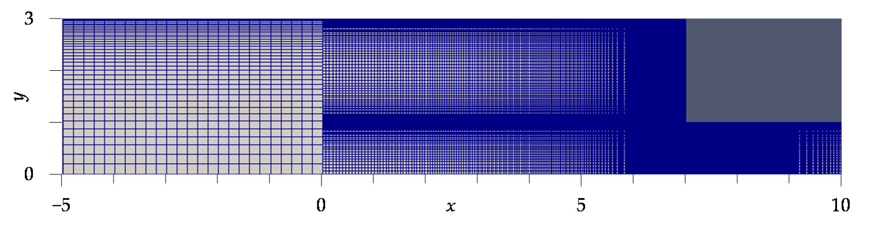
Figure 2 shows the finest mesh employed in this study. The velocity distribution of the flow suddenly changes around a corner, so the unequal interval mesh system, which is finer around two corners, has been used. For instance, even with regard to a two-dimensional cavity flow it is proved that the unequal interval mesh system gains an advantage over the uniform mesh system by a comparison of numerical errors [25]. The mesh system was designed so that its interval was finer around the two corners in the region of x0 ≤ x ≤ x2 in the mainstream x direction, as well as in the y direction such as in a turbulent channel flow. In Figure 1, the thin lines in the computational region indicate the boundary lines through which the direction of coarseness and fineness is exchanged.
As shown in Table 1, the three kinds of mesh systems, i.e., the equal interval mesh (Model A), the course unequal interval mesh (Model B), and the fine unequal interval mesh (Model C), were used. The number of the meshes (control volumes) is written as Nx (the number of the meshes in the x direction) × Ny (the number of the meshes in the y direction). The intervals of the unequal interval meshes vary in the geometric progression so that the ratio of the maximum and the minimum of them is Rx = Ry = 10. The verification of accuracy of the discretization is checked by comparing the three kinds of the meshes, which is described in Section 2.3. The following shows the results of Model C, unless otherwise specified.
In addition, the time step Δt was set so that the maximum courant number Comax was 0.3 or less by considering the numerical simulation of the plane Poiseuille flow [2]. The time step in Model C is 0.002 (Δt = 0.002), and the time step in the others is adjusted so that Comax becomes almost equal to Model C. Details of the meshes are shown in Table 1. Mainly using an Intel Xeon E3-1241 v3 (3.50 GHz × 8) for CPUs, the required time for the calculation of Model C was 12.4 days for 2000 dimensionless times at Re = 2000 with six threads paralleled.
The computational method in this study is somewhat similar to direct numerical simulation (DNS), since no turbulence models are employed. Although the present finite volume method (OpenFOAM) guarantees the conservation of physical quantities, it can only secure up to the second-order accuracy, and there is a lack of higher-order statistics. Therefore, we avoided to use the word “DNS” in this paper. However, even with this two-dimensional solver, we believe that this computational method can capture turbulent kinetic energy to some extent for the range of Reynold numbers (1200 ≤ Re ≤ 2000) where the corresponding channel flow with an expanded section is in a transitional regime between laminar and turbulent flows. Based on several previous researches on turbulent channel flows, we used a mesh system, sufficiently resolving the flows of such a range of Reynolds numbers.
This study is an extension of the research on plane Poiseuille flow and is focusing on the transition process by numerical simulation. As a matter of fact, such a study on the plane Poiseuille flow can be found in [2]. Regarding the flow in a channel with an expanded section, direct solving the two-dimensional Navier–Stokes equation without using a turbulent model has been reported [3,4,5,6,7,8,9,10,11,13,14,19]. This study followed this kind of approach.
2.3. Evaluation of Discretization Error
A space discretization error is caused by the structure or fineness of the mesh system employed, and it greatly influences the characteristics of the computational results. In this section, the space discretization error caused by a mesh size was evaluated by referring to Ferziger and Perić [25]. If targeted variables converge monotonously when a mesh size is made finer systematically, the mesh dependency is judged to be small enough. In case of using an equal-interval mesh system, it is best to make a mesh size finer by half. Although it cannot avoid that the discretization error is included in the computational results, if the targeted variables exhibit a tendency to converge monotonously, it is concluded at least that the reproducibility of the qualitative characteristics is ensured. The order of a scheme o can be obtained by Equation (6) by use of the results obtained from the three kinds of the models whose mesh size is varied systematically. Here, r is an increasing rate of a mesh size, φ is an arbitrary physical value, and l is the width of the finest mesh in the subscript in Equation (6). When the scheme order takes a positive value, the computational result converges monotonously to a true value.
For evaluating mesh dependency, the mesh size was varied at Re = 1200, where the flow oscillates periodically. For the convenience of the evaluation, the meshes are spaced equally as Δx = Δy. The three kinds of mesh size that are examined are Δx = 1/20, 1/40, and 1/80. The mesh of Δx = 1/20 is the same as that in Model A. A time step was set as Δt = 0.005. The maximum amplitude v′max of the time-fluctuating velocity component v′ was selected as the targeted physical value, which was sampled by the position at (x, y) = (10, 0.5). As a result, v′max was 0.0666, 0.0979, and 0.110 for Δx = 1/20, 1/40, and 1/80, respectively. Based on them, the scheme order was calculated as o = 1.34 by Equation (6), where r = 2, φ = v′max, and l = Δx = 1/80 were substituted. The amplitude v′max converges to a constant value, so the characteristic of the target can be reproduced enough.
Next, the influence of time steps Δt was discussed by invoking a way to evaluate the spatial discretization error. The convergence was evaluated when a time step Δt was decreased to 0.01, 0.005, and 0.0025 for a mesh interval fixed as Δx = 1/40. For the calculation of the scheme order, the smallest mesh size l was replaced with the least time step Δt = 0.0025 in Equation (6). As a result, v′max was 0.0990, 0.0979, and 0.0974 for Δt = 0.01, 0.005, and 0.0025, respectively. The scheme order was calculated as o = 1.32.
Furthermore, in order to compare the influence of the different mesh structures on the flow at Re = 2000, the dimensionless fundamental frequency f1 and its amplitude |V(f1)| of the velocity component v at (x, y) = (10, 0.5) were calculated by the discrete Fourier transform (DFT). The program of the DFT is supplied as the application [26]. When the equal interval mesh system (Model A) was used, the flow changed to chaos as soon as the computation was started at Re = 2000. On the other hand, a quasi-periodic oscillatory flow was able to be obtained with the unequal interval meshes at Re = 2000. Specifically, the results on Model C were f1 = 0.0792 and |V(f1)| = 0.0652. Even on Model B, which is courser than Model C, and whose results f1 = 0.0785 and |V(f1)| = 0.0606 are almost equal to those on Model C. Therefore, it is considered that the mesh of Model C has enough accuracy of discretization.
3. Results and Discussion
3.1. Periodic Characteristics
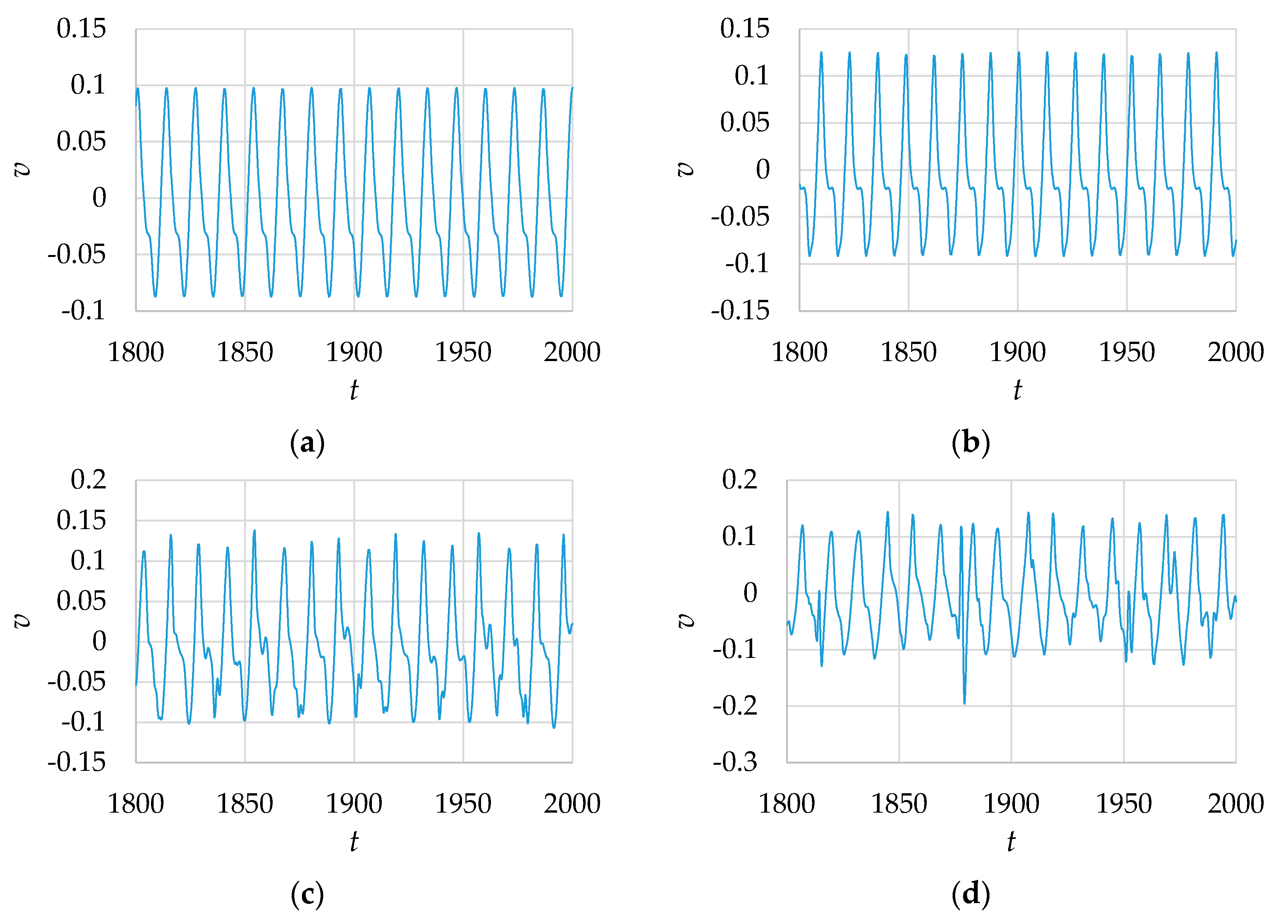
Figure 3 shows the time evolution of the velocity component v at (x, y) = (10, 0.5). The sampling position followed that of Mizushima et al. [8], and the position was slightly shifted from the channel center in order to handle both symmetric and antisymmetric disturbances at Re = 1200, as shown in Figure 3.
In order to understand the characteristics of the oscillatory flows, the amplitude spectrum of the velocity component v was created by the DFT (discrete Fourier transform). In order to set the dimensionless frequency interval to Δ, f = 0.001 when the number of samples N = 2000, and the output data for 1000 dimensionless times, t, with intervals of dimensionless times 0.5 was prepared.
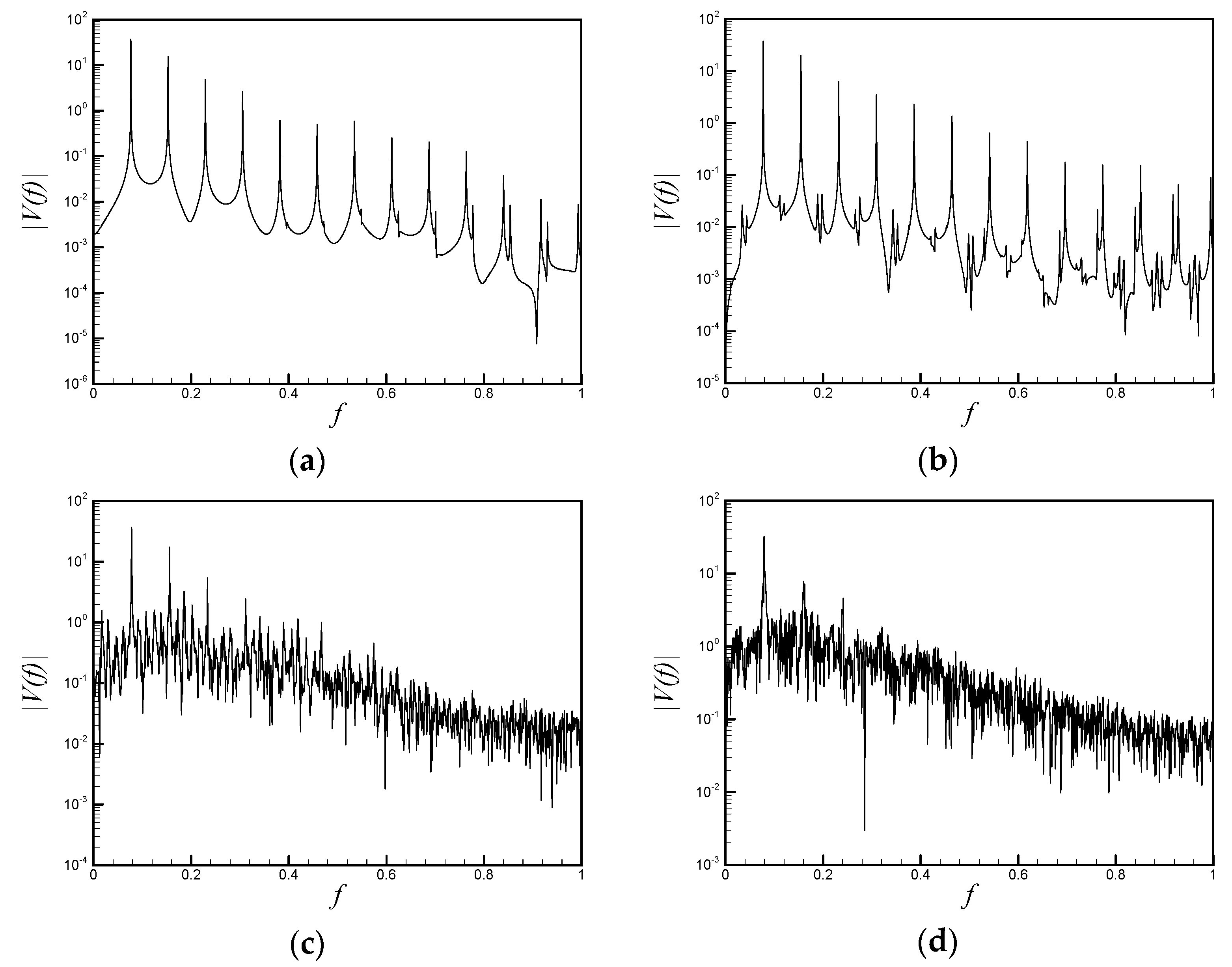
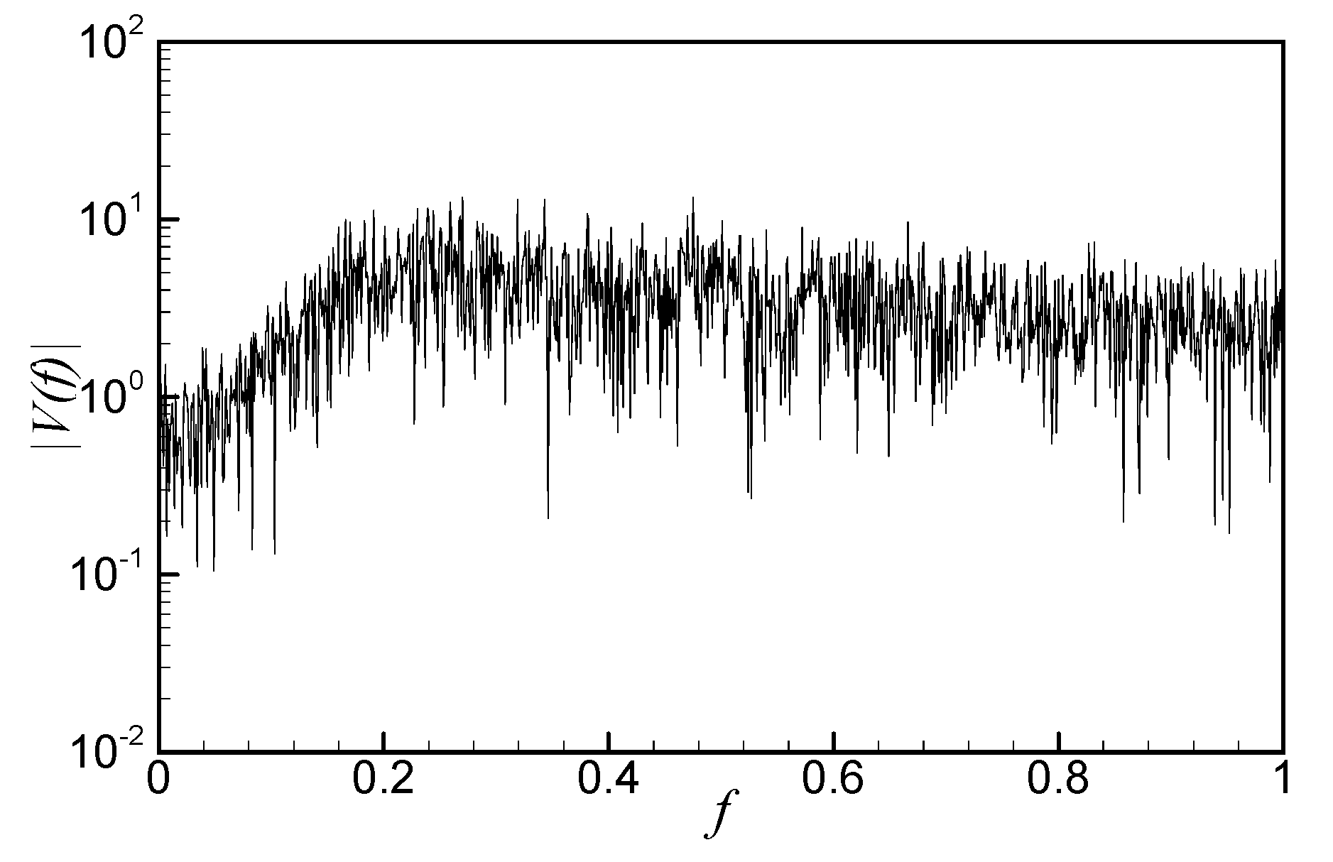
Figure 4 shows the amplitude spectrum |V(f)| of the velocity component v at (x, y) = (10, 0.5). At Re = 1200, as shown in Figure 4a, the flow is so periodic that only the peaks of the fundamental and the harmonics appear. At Re = 1400, as shown in Figure 4b, a peak is observed in the low frequency component in the order of |V(f)| ≈ 10−2; thus, it suggests that the flow transition to a quasi-periodic state having the waveform of the modulated wave takes place. In the range of Re ≥ 1600, it exhibits irregular quasi-periodic flow, as recognized from the mixing of the non-harmonic, which includes the aperiodic components for the fundamental wave. The non-harmonic increases with the Reynolds number, and at Figure 4c, where Re = 1600, only the weak non-harmonic is discretely mixed, but at Figure 4d, where Re = 2000, the non-harmonic is mixed continuously.
3.2. Vortex Generation
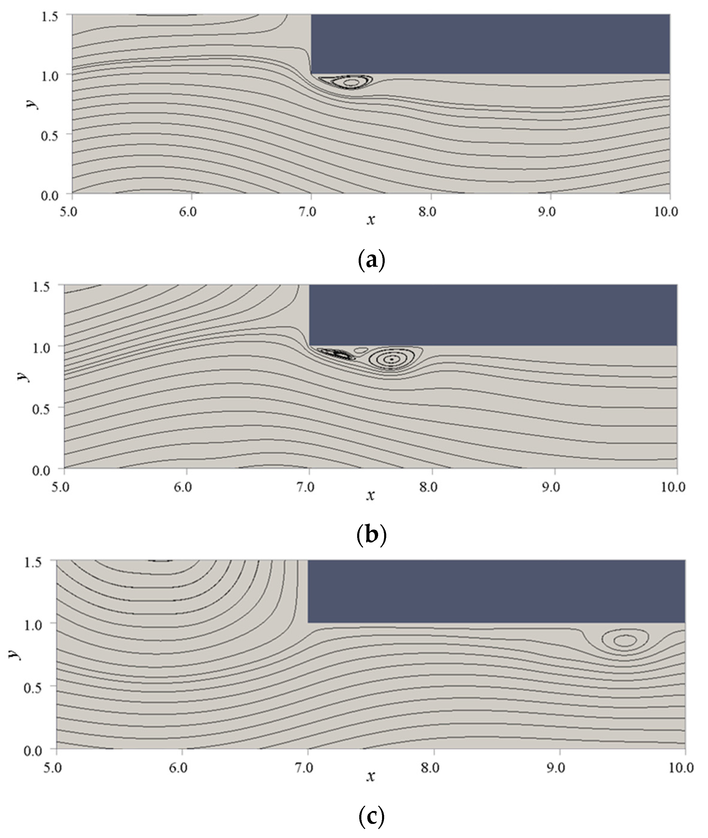
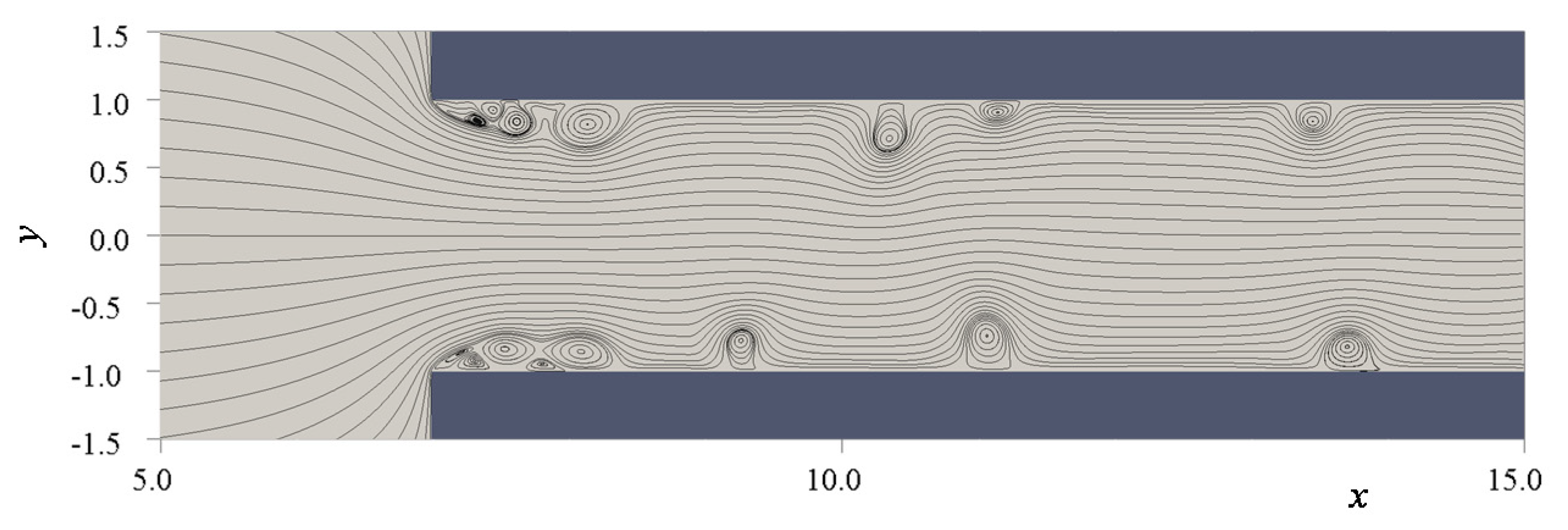
In Figure 5, the streamlines at Re = 2000 are shown. The vortices, which are caused by the oscillation of the main flow, were released from the corner of the sudden contraction part. Figure 5 is the visualization of a sequence of a process in which a group of vortices is generated and then swept downstream. The size of the vortex is not constant, and the vortex is not always continuously generated. Its reason is considered to be that the main stream at the upstream side of the sudden contraction section has been changed to the quasi-periodic oscillating flow, including the low-frequency components. Judging from the streamlines, the generation of a similar vortex was observed in Re ≥ 1600.
We consider the mechanism of how the vortex occurs in this flow, referring to Figure 5. In the following description, the part of the wavy pattern of the main stream, which is represented by the streamlines is convex in the direction of y > 0, is called the crest, and that which is convex in the direction of y < 0 is called the trough. The crest of the wave generated by the main stream oscillation cannot sometimes keep touching the wall when it passes the corner of the sudden contraction part, whereby the separation vortices are formed as shown in Figure 4a. At Re = 2000, although the vortex is usually alone, two of the additional vortices in the upstream side rarely are generated, which are very small and quickly disappear as soon as it has been generated. When the direction of the velocity becomes parallel to the wall near the corner, the growth of the separation vortices stops, and the vortices having formed by that time are swept downstream because they cannot stay just behind the sudden contraction part. The group of the vortices passes the downstream region touching the wall. The vortices occur in the downstream side of the crest of the wave, but they move in the upstream side of the crest passing the downstream region. Therefore, it appears that the phase velocity of the vortices is lower than that of the wavy pattern of the main flow.
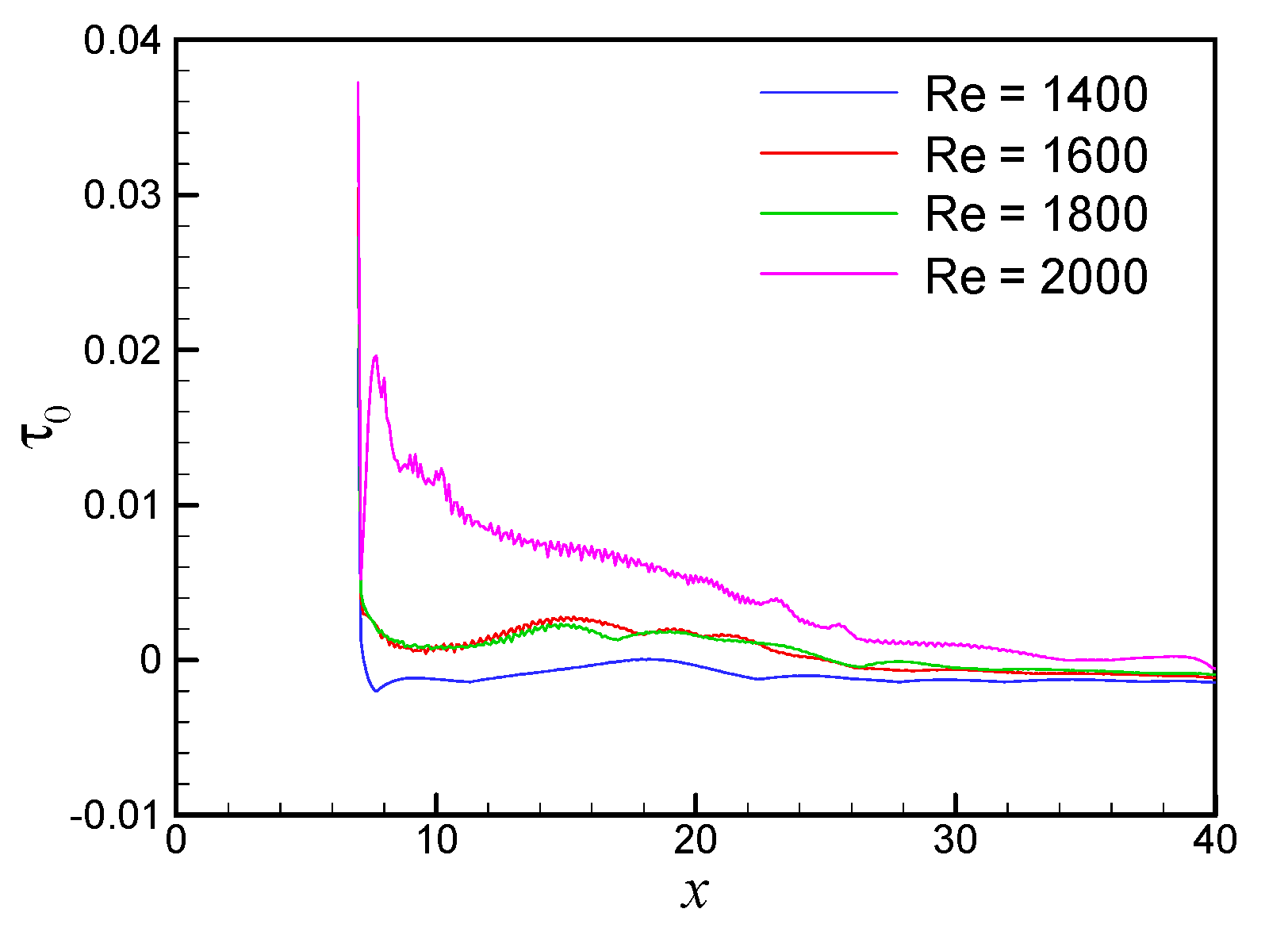
In order to identify accurately the generation of the vortex, the wall shear stress τ0 was calculated. Paying attention to the flat plate at y = 1 in the downstream region of the sudden contraction part, τ0 is defined as Equation (7), where τ0 < 0 for the region where there is no vortex. If the three vortices happen, the sign of τ0 changes twice from minus to plus when the group of the vortices passes at a sampling point.
Figure 6 is the distribution of the maximum of τ0 for t = 1000–2000. The magnitude of τ0 correlates with the size of the vortex. The maximum at Re = 2000 is clearly larger than one in Re ≤ 1800 because the much bigger groups of the vortices have been generated several times during the computation.
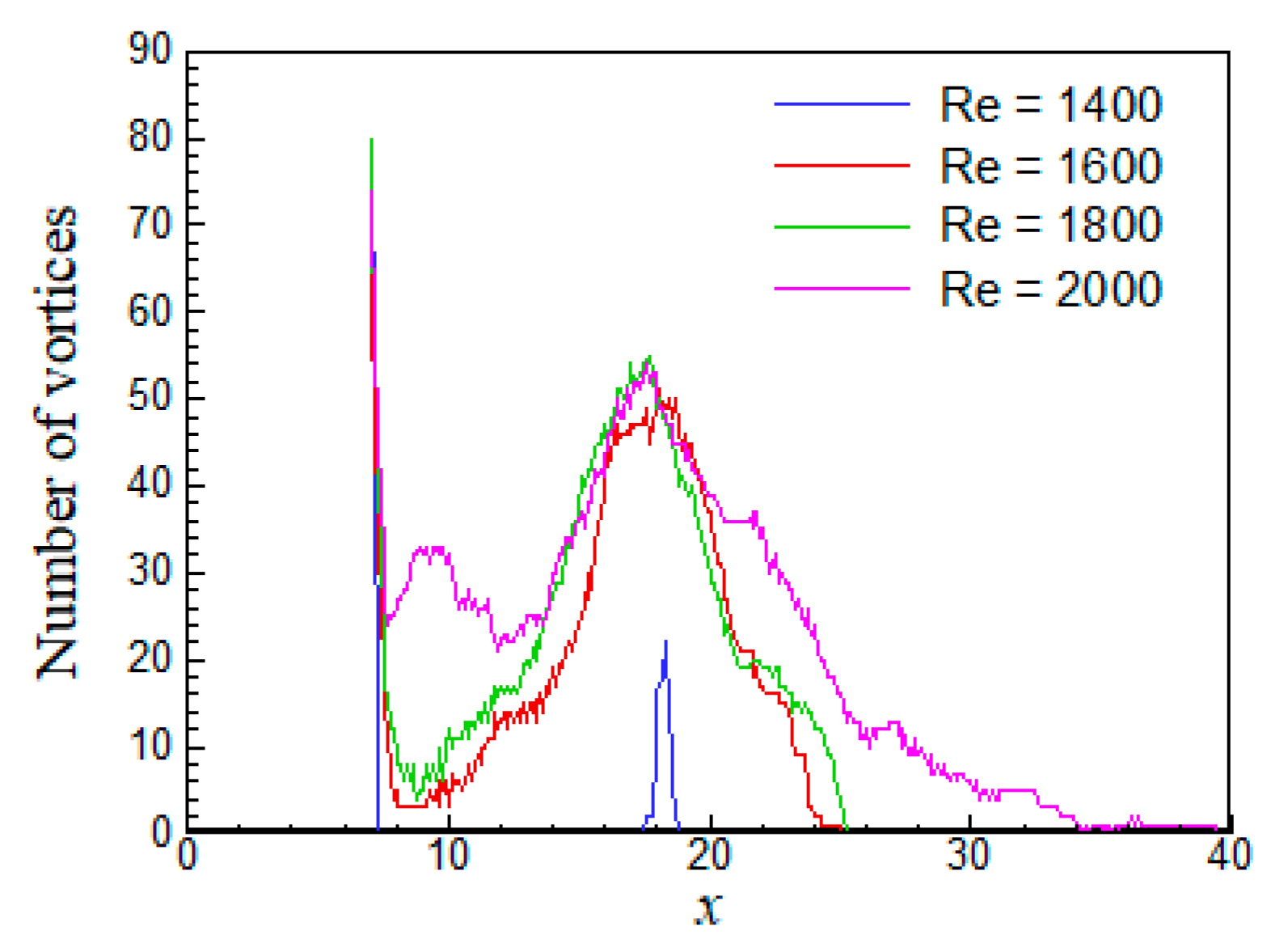
Figure 7 represents the number that the vortex has generated, which is obtained by counting the times that the wall shear stress changes from minus to plus. If one vortex is made in each period, the vortices of about 79 are generated for t = 1000–2000 because of the fundamental frequency f1 ≈ 0.079. Most of the vortices disappear just behind the sudden contraction part (x ≈ 7) as soon as they are generated, but the vortices are generated again in the downstream region, and the number of them is at a maximum near x ≈ 18. Note that the sign reversal occurs more than 70 times at x = 7, since a part of the main flow passing through the sudden contraction part flows backward, and it joins up with the circulation vortex in the upstream region of the expanded section when the flow pattern of the stream line changes from a crest to a trough.
The mechanism of the vortex generation described in the above paragraph is held regardless of the periodicity of the oscillating flow. Therefore, although the scale and generation period of the vortex are affected by the periodic characteristics of the oscillating flow, the vortex can occur whether the oscillating flow is periodic or aperiodic. Conversely, there is a possibility that the generation of vortices affects the periodicity of the oscillating flow. In addition, there is also another possibility that an aperiodic component on the sudden contraction part affects upstream owing to the transport by the circular vortex in the cavity. These two possibilities are discussed in the following subsections.
3.3. Effect of a Sudden Contraction Part
In the above section, we observed the two phenomena such as the non-periodic flow and the vortex generation. These phenomena are also observed in the flow between parallel plates with only a sudden reduction part. The flow in the channel with a sudden contraction part was simulated in the same way as that in the channel with the suddenly expanded section, and then the relationship between the two was investigated. In the channel flow with the sudden contraction part, a separation region is formed immediately after the suddenly contracted part. Such a flow is called a separation flow. In addition, there is another separation flow that occurs at the leading edge of a thick plate [27] or a blunt cylinder [28], for which the oscillatory characteristics have been investigated experimentally. As a common feature of the separation flow, the vortex shedding from the separation region takes place. The spectrum is continuous, and the central frequency ranges from 0.5 to 0.8 times the frequency defined by the characteristic velocity and length [29].
In the computation of the channel flow with the sudden contraction part, the mesh system was designed so as to be almost the same as that of the flow in the channel with the suddenly expanded section. The details are shown in Table 2. The location of sudden contraction was set at x = 7 and the reduction ratio was set at Cn = Ex = 3, which are the same values as those for the flow in the channel with the suddenly expanded section. The computational area (−20 ≤ x ≤ 40) was taken so long as it was not affected by the entrance boundary conditions. Using a non-matching mesh system in which meshes with different intervals are joined together at interfaces between the two different sub mesh systems, the computational time was attempted to be shortened. Figure 8 shows a mesh system for Model E, which has the same mesh structure as Model C shown in Table 1 for the region 0 ≤ x ≤ 40. In the qualitative evaluation stage, a coarse mesh system (Model D) was used.
Chiang and Sheu [30] reported that a bifurcation from a symmetric flow to an asymmetric flow occurred by carrying out a two-dimensional steady computation for the flow in suddenly reducing channels. The critical Reynolds number Rec varied with the reduction ratio Cn, and such values were Rec = 2310 (Cn = 2), 1013 (Cn = 4), and 825 (Cn = 8). Judging from this tendency, the critical Reynolds number at Cn = 3 was expected to be 1013 < Rec < 2310. The present time-marching computations implemented using a Model E mesh system gave an asymmetric steady flow at Re = 2000 and an irregular unsteady flow at Re = 4000. The channel flow with the sudden contraction part immediately changed from a steady state to a time-dependent irregular state as the Reynolds number increases. Although Model F was also carried out for Re = 4000, it took a very long computational time; therefore, we just confirmed that there was no significant difference in the vortex generation pattern between Model E and Model F.
Figure 9 shows streamlines obtained with Model F for Re = 4000. In the channel flow with the sudden contraction part, the separation region is formed because the fluid cannot follow the wall surface of a corner. The separation region contains multiple vortices. The vortices are created continuously from the corners, the vortex created earlier is pushed downstream, and eventually the most downstream vortex breaks down and is moved further downstream. The breakdown position is in the vicinity of the reattachment point of the separation region, which is recognized by seeing the time-averaged field. A similar vortex generation and breakdown mechanism has been reported in experiments for a leading-edge separation flow [29]. The size of the vortex is almost the same, but the period of the vortex breakdown varies considerably. In the leading-edge separation of a blunt cylinder, the pressure and the velocity fluctuation spectra at the reattachment position exhibit continuous and wide peaks [28].
In order to compare the aperiodic characteristics, the amplitude spectrum |V(f)| of the flow in the channel with the sudden contraction part at Re = 4000 is shown in Figure 10. The mesh system of Model E was used. In addition to the position at (x, y) = (10, 0.5), an amplitude spectrum at (x, y) = (10, −0.5) was also investigated, and it was confirmed that there were no differences between the two spectra. Since the Reynolds numbers are different from each other, the amplitudes cannot be compared fairly, but the distribution seems such that only the non-harmonic component is extracted from the spectrum of the flow in the channel with the suddenly expanded section at Re = 2000, as shown in Figure 4d. There are no discrete peaks in the spectrum, but it takes its maximum at f ≈ 0.2, assuming an approximated curve of the spectrum.
The characteristics of the aperiodic oscillatory flow with the sudden contraction part are compared with those in the channel with the suddenly expanded section. In the flow in the channel with the sudden contraction part, an aperiodicity of the flow is generated by the breakdown of the separation region. On the other hand, in the channel flow with the suddenly expanded section, the vortex generation is linked to the periodic oscillation of the main flow, so the characteristics of the two flows are different. In addition, there is no mechanism of transporting aperiodicity upstream in the channel flow with the sudden contraction part, unlike the circulating vortex observed in the channel flow with the suddenly expanded section. Therefore, the aperiodic oscillatory flow in the channel flow with the sudden contraction part is different from that in the channel flow with the suddenly expanded section, although they have the common features of aperiodicity and vortex generation.
In a contraction channel, the smaller the reduction ratio, the higher the critical Reynolds number for a transition from symmetric flow to asymmetric flow. The critical Reynolds number to take a transition from steady flow to unsteady flow is considered to be the same tendency. With regard to a partially expansion channel, in which there are few papers that systematically investigated the effects of the expansion/contraction ratio, it would be expected that the critical Reynolds number for the transition from steady flow to non-steady flow may increase.
3.4. Turbulent Kinetic Energy
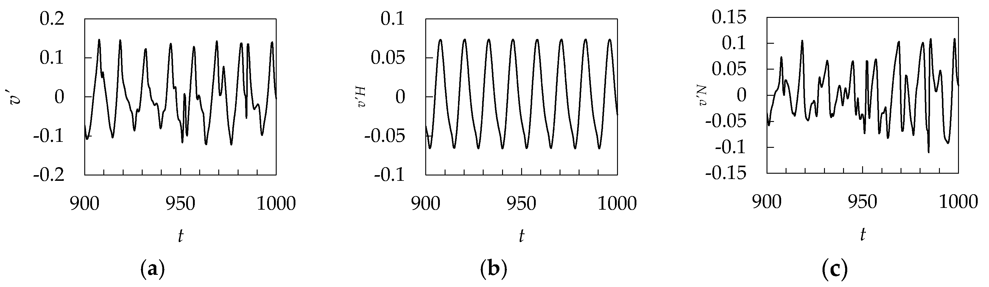
It was attempted to extract only aperiodicity from oscillation characteristics. In order to specify where the aperiodic component composed in the amplitude spectrum was made, the time-fluctuating velocity components u′, v′ were decomposed into the harmonics u′H, v′H and the non-harmonics u′N, v′N, as shown in Equation (8) and Figure 11.
where the subscript H and N symbolizes the harmonics (periodic components) and the non-harmonics (aperiodic components).
To be more specific, the time-fluctuating velocity component u′ is restored from the output of the DFT as follows. The other component v′ is likewise.
The subscript numbers i = 0, 1, 2, …, N − 1 are defined by using the number of sample N. The term of i = 0 is the time-mean velocity component ū. With respect to the discrete frequency fi = i/(NΔt) of the number i based on the sampling period Δt = 0.5, the amplitude ai and the phase θi are obtained as 1/N times the absolute value and the argument of the complex numbers obtained with the DFT. Then, assuming that the components of the m-th harmonic (m = 1, 2, …) are fm, am and θm, the harmonic component u′H is defined by Equation (10).
Note that the range of the sum of the harmonic components is 0 < f < fc considering the Nyquist frequency fc = 1/(2Δt). Moreover, the relation that cos(2πfit + θi) = cos(2πfN−it + θN−i) is valid by the symmetries for the Nyquist frequency of the DFT and the trigonometric function, so each harmonic component is doubled.
The turbulent kinetic energy k, a harmonic component kH, and a non-harmonic component kN are defined as shown in Equations (11)–(13), where , , , , , are obtained by the arithmetic mean of the time-fluctuating velocity component.
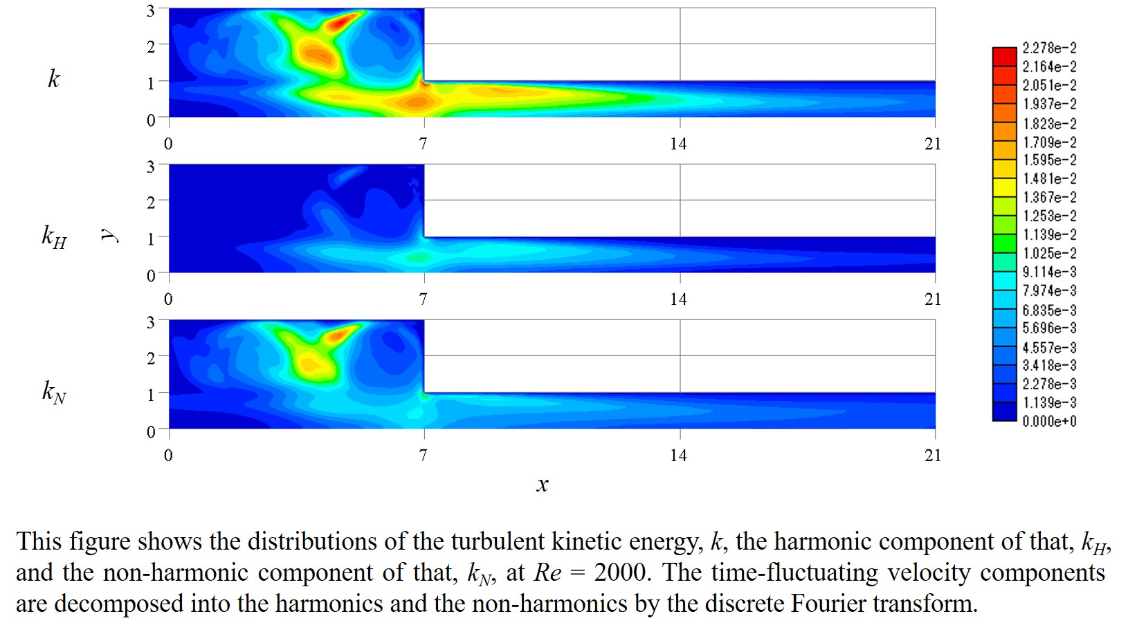
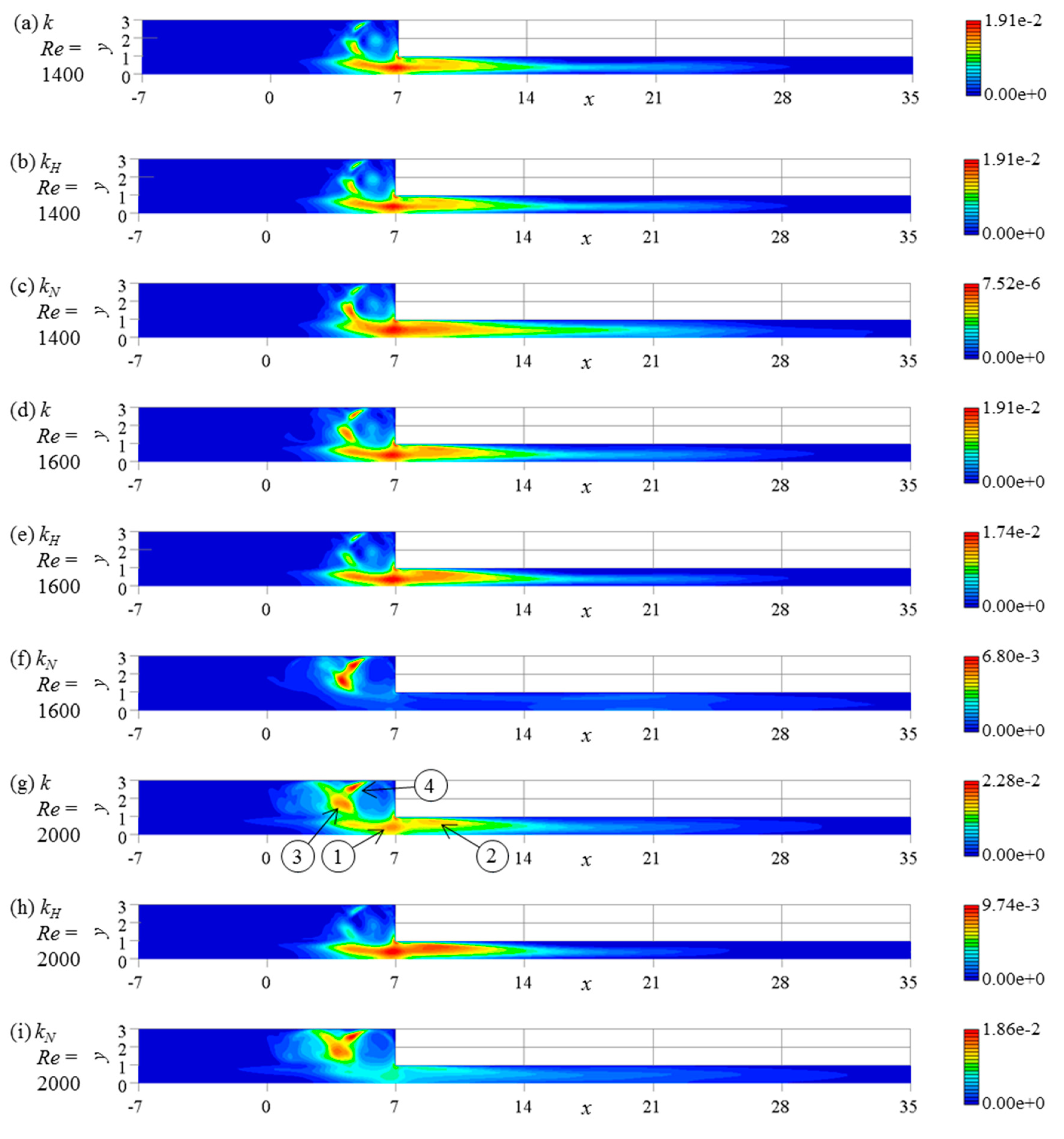
As shown in Figure 12, the distributions within the x–y plane (−7 ≤ x ≤ 35, 0 ≤ y ≤ 3) were made in regard to the turbulent kinetic energy k, kH, and kN. At Re = 1400, the flow is almost periodic, having the waveform of the modulated wave, so the patterns of three components are similar to each other. When the flow is quasi-periodic as shown in the cases at Re = 1600 and Re = 2000, the patterns are different between the harmonics kH and the non-harmonics kN, but the position of a peak does not tend to be changed irrespective of the Reynolds number.
Concerning the maximum value of the kinetic energy, the maximum value of kN is less than 1% compared with that of kH at Re = 1400, but both have the same order maximum value for Re = 1600. At Re = 2000, the maximum value of kN is larger than that of kH.
The harmonic and non-harmonic components are both attenuated in the downstream area after passing the sudden contraction section. This can be recognized from the contour diagram in Figure 12. This is because Re = 2000 is below the critical Reynolds number of the plane Poiseuille flow predicted by weak non-linear stability analysis [1]. The flow at x = 35 is stable, since this position is sufficiently far from the sudden contraction part.
Judging from the distribution of the turbulent kinetic energy k, the four peaks where k takes locally its maximum are identified except near the corners. These are indicated by the arrows together with corresponding numbers, as shown in Figure 12g. The first peak is located at the center of the channel near the sudden contraction position (x ≈ 7, y = 0). The second one stretches out from the corner of the sudden contraction part. The third and fourth ones are observed near the contact positions between two circular vortices in the expanded section.
The first peak is caused by the main stream oscillation becoming excited in the suddenly expanded section and attenuated in the downstream of the sudden contraction part. This is a periodic phenomenon, because the harmonic component kH is dominant. Its fundamental wave is the antisymmetric disturbance, because the velocity component u is an odd function and v is an even function. Therefore, the maximum value of the peak does not exist at y = 0, which is the center line of the channel, but it exists at y ≈ 0.5.
The second peak is due to the action of backward flow near the wall just after the sudden contraction part. In fact, the separation vortices are formed actively when Re ≥ 1600. This is also mainly recognized as the harmonic component kH.
The third and fourth peaks are recognized as the non-harmonic component kN unlike the cases mentioned above. Therefore, it can be seen that the aperiodicity of the flow is generated not in the downstream of the sudden contraction part but in the expanded section on the upstream side of the corner. Although the region where kN becomes apparent is limited, kN spreads slightly to the downstream, and it appears clearly that the change of the vortices size is observed just after the sudden contraction.
As stated above, there are the peaks of the non-harmonic component kN near the contact of the vortices in the expanded section. That is, it is considered that the flow aperiodicity is an inherent property for the expanded section, and it is caused by the interaction of the circular vortices at a certain Reynolds number or more. The circular vortex hardly transports the non-harmonic component from the sudden contraction part. In addition, no conspicuous peak has been observed in the non-harmonic component of the turbulent kinetic energy in the downstream of the sudden contraction part, so the separation vortex does not significantly affect the aperiodic oscillating flow. Therefore, the aperiodicity of flow and the generation of vortices occur independently, although they are interacted with each other. Since the generation of the separation vortices did not always occur, it would be a secondary phenomenon that occurs irregularly.
4. Conclusions
In this study, the two-dimensional numerical simulation was carried out for the oscillating flow between the parallel flat plates with the suddenly expanded section whose expansion ratio is 3 and aspect ratio is 7/3. Although the present results should be corroborated in a future challenging experiment or in a three-dimensional numerical simulation, the following conclusions were obtained.
- At the Reynolds number Re = 1200, it is the periodic oscillating flow. At Re = 1400, it becomes the quasi-periodic oscillating flow having the waveform of the modulated wave, which includes the low-frequency components. In Re ≥ 1600, it is the quasi-periodic oscillating flow with the disordered fluctuations.
- For Re ≥ 1600, the separation vortices are sometimes generated because the wave crest caused by the oscillating main flow cannot keep touching the wall before it passes the corner of the sudden contraction part. Furthermore, the size of the vortex is not constant, and the vortex is not always generated. Most of the vortices disappear just behind the sudden contraction, but the vortex appears again in the downstream region.
- When the turbulent kinetic energy is decomposed into the harmonic component and the non-harmonic component, the peaks of the non-harmonic component are localized near the contact of the vortices in the expanded section. That is, the aperiodic characteristics of the oscillating flow are generated in the expanded section. The circular vortex hardly transports the non-harmonic component from the sudden contraction part.
- The aperiodicity of flow and the generation of vortices interact with each other, but each phenomena occurs independently. It has been exhibited that the aperiodicity of flow is hardly affected by vortex generation, since the peak of the non-harmonic component of turbulent energy exists in the expanded region.
Author Contributions
Conceptualization, T.M.; Data curation, T.M.; Formal analysis, T.M.; Investigation, T.M.; Methodology, T.M.; Software, T.M.; Supervision, T.T.; Visualization, T.M. and T.T.; Writing—original draft, T.M.; Writing—review & editing, T.T.
Funding
This research received no external funding.
Conflicts of Interest
The authors declare no conflict of interest.
Nomenclature
| As | aspect ratio [-] |
| Cn | contraction ratio [-] |
| Comax | maximum courant number [-] |
| Ex | expansion ratio [-] |
| f | dimensionless frequency = f*δ*/U* [-] |
| f* | frequency [Hz] |
| f1 | dimensionless fundamental frequency [-] |
| k | dimensionless turbulent kinetic energy [-] |
| N | number of samples on discrete Fourier transform [-] |
| Nx | number of meshes in the x direction [-] |
| Ny | number of meshes in the y direction [-] |
| p | dimensionless pressure = p*/ρ*U*2 [-] |
| p* | pressure [Pa] |
| Rx | ratio of the maximum and the minimum of meshes in the x direction [-] |
| Ry | ratio of the maximum and the minimum of meshes in the y direction [-] |
| Re | Reynolds number = U*δ*/ν* [-] |
| Rec | critical Reynolds number [-] |
| t | dimensionless time = t*U*/δ* [-] |
| t* | time [s] |
| u | dimensionless velocity vector = (u, v) [-] |
| u | dimensionless x-directional velocity component = u*/U* [-] |
| u* | x-directional velocity component [m/s] |
| U* | characteristic velocity as the maximum of the plane Poiseuille flow [m/s] |
| Uc | advection velocity [-] |
| v | dimensionless y-directional velocity component = v*/U* [-] |
| v* | y-directional velocity component [m/s] |
| v′ | dimensionless time-fluctuating velocity component of v [-] |
| v′max | dimensionless maximum amplitude of v′ [-] |
| |V(f)| | dimensionless amplitude spectrum of v [-] |
| x | dimensionless coordinate vector = (x, y) [-] |
| x | dimensionless x coordinate = x*/δ* [-] |
| x* | x coordinate [m] |
| y | dimensionless y coordinate = y*/δ* [-] |
| y* | y coordinate [m] |
| Greek Symbols | |
| Δf | dimensionless frequency interval on discrete Fourier transform [-] |
| Δt | dimensionless time step [-] |
| Δx | dimensionless mesh size in the x direction [-] |
| Δy | dimensionless mesh size in the y direction [-] |
| δ* | characteristic length as the half height of the channel [m] |
| ν* | coefficient of kinetic viscosity [m2/s] |
| ρ* | density [kg/m3] |
| τ0 | dimensionless wall shear stress on the upper wall = τ0*/ρ*U*2 [-] |
| τ0* | wall shear stress on the upper wall [Pa] |
| Subscripts or Superscripts | |
| * | dimension values |
| ¯ | time-mean |
| ′ | time-fluctuating |
| H | harmonics (periodic components) |
| N | non-harmonics (aperiodic components) |
References
- Ehrenstein, U.; Koch, W. Three-dimensional wavelike equilibrium states in plane Poiseuille flow. J. Fluid Mech. 1991, 228, 111–148. [Google Scholar] [CrossRef]
- Jiménez, J. Transition to turbulence in two-dimensional Poiseuille flow. J. Fluid Mech. 1990, 218, 265–297. [Google Scholar] [CrossRef]
- Ghaddar, N.K.; Korczak, K.Z.; Mikic, B.B.; Patera, A.T. Numerical investigation of incompressible flow in grooved channels. Part 1. Stability and self-sustained oscillations. J. Fluid Mech. 1986, 163, 99–127. [Google Scholar] [CrossRef]
- Nishimura, T.; Morega, A.M.; Kunitsugu, K. Vortex structure and fluid mixing in pulsatile flow through periodically grooved channels at low Reynolds numbers. JSME Int. J. Ser. B 1997, 40, 377–385. [Google Scholar] [CrossRef]
- Adachi, T.; Hasegawa, S. Transition of the flow in a symmetric channel with periodically expanded grooves. Chem. Eng. Sci. 2006, 61, 2721–2729. [Google Scholar] [CrossRef]
- Adachi, T.; Uehara, H. Transitions and pressure characteristics of flow in channel with periodically contracted-expanded parts. Trans. Jpn. Soc. Mech. Eng. Ser. B 2001, 67, 52–59. [Google Scholar] [CrossRef]
- Takaoka, M.; Sano, T.; Yamamoto, H.; Mizushima, J. Transition and convective instability of flow in a symmetric channel with spatially periodic structures. Phys. Fluids 2009, 21, 1–10. [Google Scholar] [CrossRef]
- Mizushima, J.; Okamoto, H.; Yamaguchi, H. Stability of flow in a channel with a suddenly expanded part. Phys. Fluids 1996, 8, 2933–2942. [Google Scholar] [CrossRef]
- Kunitsugu, K.; Nishimura, T. The transition process of pulsatile flow in grooved channel at intermediate Reynolds number (effect of groove length). Trans. Jpn. Soc. Mech. Eng. Ser. B 2006, 72, 3074–3081. [Google Scholar] [CrossRef]
- Sahan, R.A.; Liakopoulos, A.; Gunes, H. Reduced dynamical models of nonisothermal transitional grooved-channel flow. Phys. Fluids 1997, 9, 551–565. [Google Scholar] [CrossRef]
- Ghaddar, N.K.; Magen, M.; Mikic, B.B.; Patera, A.T. Numerical investigation of incompressible flow in grooved channels. Part 2. Resonance and oscillatory heat-transfer enhancement. J. Fluid Mech. 1986, 168, 541–567. [Google Scholar] [CrossRef]
- Greiner, M. An experimental investigation of resonant heat transfer enhancement in grooved channels. Int. J. Heat Mass Transf. 1991, 34, 1383–1391. [Google Scholar] [CrossRef]
- Roberts, E.P.L.; Mackley, M.R. The development of asymmetry and period doubling for oscillatory flow in baffled channels. J. Fluid Mech. 1996, 328, 19–48. [Google Scholar] [CrossRef]
- Okamoto, H.; Mizushima, J.; Yamaguchi, H. Stability of pipe flow with sudden expansion and wave propagation. RIMS Kôkyûroku 1996, 949, 128–138. [Google Scholar]
- Cornejo, I.; Nikrityuk, P.; Hayes, R.E. Pressure correction for automotive catalytic converters: A multi-zone permeability approach. Chem. Eng. Res. Des. 2019, 147, 232–243. [Google Scholar] [CrossRef]
- Lambert, C.; Chanko, T.; Dobson, D.; Liu, X.; Pakko, J. Gasoline particle filter development. Emiss. Control Sci. Technol. 2017, 3, 105–111. [Google Scholar] [CrossRef]
- Liou, T.M.; Lin, C.T. Study on microchannel flows with a sudden contraction–expansion at a wide range of Knudsen number using lattice Boltzmann method. Microfluid. Nanofluidics 2014, 16, 315–327. [Google Scholar] [CrossRef]
- Makino, S.; Iwamoto, K.; Kawamura, H. Turbulent structures and statistics in turbulent channel flow with two-dimensional slits. Int. J. Heat Fluid Flow 2008, 29, 602–611. [Google Scholar] [CrossRef]
- Murakami, S.; Mizushima, J. Stability and transitions of flow in a channel with a suddenly expanded part. RIMS Kôkyûroku 2012, 1800, 184–194. [Google Scholar]
- The OpenFOAM Foundation, Download v2.3.1|Ubuntu. Available online: https://openfoam.org /download/2-3-1-ubuntu/ (accessed on 16 February 2019).
- Rojas, E.S.; Mullin, T. Finite-amplitude solutions in the flow through a sudden expansion in a circular pipe. J. Fluid Mech. 2012, 691, 201–213. [Google Scholar] [CrossRef]
- Sakurai, M.; Nakanishi, S.; Osaka, H. Three-dimensional structure of laminar flow through a square sudden expansion channel (vortex structure of the recirculation zone). Trans. Jpn. Soc. Mech. Eng. Ser. B 2013, 79, 317–327. [Google Scholar] [CrossRef]
- Sakurai, M.; Nakanishi, S.; Osaka, H. Three-dimensional structure of laminar flow through a square sudden expansion channel (effect of Reynolds number). Trans. Jpn. Soc. Mech. Eng. Ser. B 2013, 79, 1533–1545. [Google Scholar] [CrossRef]
- Kasuga, Y.; Imano, M. Numerical Analysis of Heat Transfer and Flow by OpenFOAM, 1st ed.; The Open CAE Society of Japan, Ed.; Morikita Publishing: Tokyo, Japan, 2016; p. 139. [Google Scholar]
- Ferziger, J.H.; Perić, M. Computational Methods for Fluid Dynamics, 1st ed.; Springer: Tokyo, Japan, 2003; pp. 199–201, 326–329. [Google Scholar]
- Kimura, S. Discrete Fourier. Available online: https://www.vector.co.jp/soft/winnt/business/se503214.html (accessed on 11 March 2019).
- Kiya, K.; Sasaki, K. Structure of a turbulent separation bubble. J. Fluid Mech. 1983, 137, 83–113. [Google Scholar] [CrossRef]
- Kiya, M.; Nozawa, T. Turbulence structure in the leading-edge separation zone of a blunt circular cylinder. Trans. Jpn. Soc. Mech. Eng. Ser. B 1987, 53, 1183–1189. [Google Scholar] [CrossRef]
- Kiya, M. Turbulence structure of separated-and-reattaching flows. Trans. Jpn. Soc. Mech. Eng. Ser. B 1989, 55, 559–564. [Google Scholar] [CrossRef]
- Chiang, T.P.; Sheu, T.W.H. Bifurcations of flow through plane symmetric channel contraction. J. Fluids Eng. 2002, 124, 444–451. [Google Scholar] [CrossRef]
Figure 1.
Channel geometry and coordinates.

Figure 2.
Mesh structure of the finest mesh, Model C. This picture shows the range of 6 ≤ x ≤ 8 and 0.8 ≤ y ≤ 1.2.
Figure 2.
Mesh structure of the finest mesh, Model C. This picture shows the range of 6 ≤ x ≤ 8 and 0.8 ≤ y ≤ 1.2.

Figure 3.
Time evolution of the velocity component v at (x, y) = (10, 0.5). (a) It was a periodic oscillating flow. At Re = 1400, as shown in (b), the local maximum is not constant, so it is a quasi-periodic oscillating flow with a modulated wave containing low frequency components. At Re = 1600, as shown in (c), in addition to having a waveform of a modulated wave, it is a quasi-periodic oscillating flow with irregular fluctuations. At Re = 2000, as shown in (d), the irregularity becomes even stronger.

Figure 4.
Amplitude spectrum |V(f)| of the velocity component v at (x, y) = (10, 0.5). (a) Re = 1200. (b) Re = 1400. (c) Re = 1600. (d) Re = 2000.
Figure 4.
Amplitude spectrum |V(f)| of the velocity component v at (x, y) = (10, 0.5). (a) Re = 1200. (b) Re = 1400. (c) Re = 1600. (d) Re = 2000.

Figure 5.
Stream lines at Re = 2000, which represent the evolution process of a group of vortices. (a) t = 1531. (b) t = 1533. (c) t = 1538.
Figure 5.
Stream lines at Re = 2000, which represent the evolution process of a group of vortices. (a) t = 1531. (b) t = 1533. (c) t = 1538.

Figure 6.
Maximum of the wall shear stress τ0 at y = 1 during t = 1000–2000.

Figure 7.
Number of the vortices coming into contact with the wall at y = 1 during t = 1000–2000.

Figure 8.
Mesh structure of the non-matching mesh for Model E. This picture shows the range of −5 ≤ x ≤ 10 and 0 ≤ y ≤ 3.
Figure 8.
Mesh structure of the non-matching mesh for Model E. This picture shows the range of −5 ≤ x ≤ 10 and 0 ≤ y ≤ 3.

Figure 9.
Stream lines in the channel with the sudden contraction part at Re = 4000 at a certain moment.
Figure 9.
Stream lines in the channel with the sudden contraction part at Re = 4000 at a certain moment.

Figure 10.
Amplitude spectrum |V(f)| of the velocity component v in the channel with the sudden contraction part at (x, y) = (10, 0.5) at Re = 4000.
Figure 10.
Amplitude spectrum |V(f)| of the velocity component v in the channel with the sudden contraction part at (x, y) = (10, 0.5) at Re = 4000.

Figure 11.
The time-fluctuating velocity component v′, which was decomposed into the harmonic v′H and the non-harmonic v′N at (x, y) = (10, 0.5). (a) Fluctuation. (b) Harmonic. (c) Non-harmonic.
Figure 11.
The time-fluctuating velocity component v′, which was decomposed into the harmonic v′H and the non-harmonic v′N at (x, y) = (10, 0.5). (a) Fluctuation. (b) Harmonic. (c) Non-harmonic.

Figure 12.
Distributions of the turbulent kinetic energy k, which is decomposed into the harmonic component kH and the non-harmonic component kN.
Figure 12.
Distributions of the turbulent kinetic energy k, which is decomposed into the harmonic component kH and the non-harmonic component kN.


Table 1.
Mesh details.
| Name | Nx × Ny | Rx, Ry | Δt | ||
|---|---|---|---|---|---|
| −20 ≤ x ≤ −7 | −7 ≤ x ≤ 7 | 7 ≤ x ≤ 40 | |||
| Model A | 260 × 40 | 280 × 120 | 660 × 40 | 1 | 0.005 |
| Model B | 117 × 46 | 224 × 138 | 479 × 46 | 10 | 0.0025 |
| Model C | 195 × 76 | 373 × 228 | 798 × 76 | 10 | 0.002 |
Table 2.
Mesh details of the channels with the sudden contraction part.
| Name | Nx × Ny | Rx, Ry | Δt | |||
|---|---|---|---|---|---|---|
| −20 ≤ x ≤ 0 | 0 ≤ x ≤ 7 | 7 ≤ x ≤ 20 | 20 ≤ x ≤ 40 | |||
| Model D | 180 × 138 | 161 × 138 | 299 × 46 | 180 × 46 | 10 | 0.0025 |
| Model E | 100 × 76 | 268 × 228 | 498 × 76 | 300 × 76 | 10 | 0.002 |
| Model F | 100 × 76 | 451 × 384 | 838 × 128 | 300 × 76 | 10 | 0.001 |
© 2019 by the authors. Licensee MDPI, Basel, Switzerland. This article is an open access article distributed under the terms and conditions of the Creative Commons Attribution (CC BY) license (http://creativecommons.org/licenses/by/4.0/).
Share and Cite
MDPI and ACS Style
Masuda, T.; Tagawa, T. Quasi-Periodic Oscillating Flows in a Channel with a Suddenly Expanded Section. Symmetry 2019, 11, 1403. https://0-doi-org.brum.beds.ac.uk/10.3390/sym11111403
AMA Style
Masuda T, Tagawa T. Quasi-Periodic Oscillating Flows in a Channel with a Suddenly Expanded Section. Symmetry. 2019; 11(11):1403. https://0-doi-org.brum.beds.ac.uk/10.3390/sym11111403
Chicago/Turabian StyleMasuda, Takuya, and Toshio Tagawa. 2019. "Quasi-Periodic Oscillating Flows in a Channel with a Suddenly Expanded Section" Symmetry 11, no. 11: 1403. https://0-doi-org.brum.beds.ac.uk/10.3390/sym11111403
Note that from the first issue of 2016, this journal uses article numbers instead of page numbers. See further details here.