Article

Normal-G Class of Probability Distributions: Properties and Applications

by
Fábio V. J. Silveira
1,
Frank Gomes-Silva
1,*,
Cícero C. R. Brito
2,
Moacyr Cunha-Filho
1,
Felipe R. S. Gusmão
1 and
Sílvio F. A. Xavier-Júnior
3
1
Department of Statistics and Informatics, Rural Federal University of Pernambuco, Recife 52171900, Pernambuco, Brazil
2
Federal Institute of Education, Science and Technology of Pernambuco, Recife 50740545, Pernambuco, Brazil
3
Department of Statistics, Paraíba State University, Campina Grande 58429500, Paraíba, Brazil
*
Author to whom correspondence should be addressed.
Submission received: 28 September 2019 / Revised: 22 October 2019 / Accepted: 12 November 2019 / Published: 15 November 2019

Abstract

:
In this paper, we propose a novel class of probability distributions called Normal-G. It has the advantage of demanding no additional parameters besides those of the parent distribution, thereby providing parsimonious models. Furthermore, the class enjoys the property of identifiability whenever the baseline is identifiable. We present special Normal-G sub-models, which can fit asymmetrical data with either positive or negative skew. Other important mathematical properties are described, such as the series expansion of the probability density function (pdf), which is used to derive expressions for the moments and the moment generating function (mgf). We bring Monte Carlo simulation studies to investigate the behavior of the maximum likelihood estimates (MLEs) of two distributions generated by the class and we also present applications to real datasets to illustrate its usefulness.

1. Introduction

For many purposes, statistical distributions are used in a plethora of science fields. They are regularly useful tools to describe natural and social phenomena, providing suitable models which can help dealing with real problems, such as for instance, those concerning the prediction of an event of interest. Recent works have focused attention at formulating and describing new classes of probability distributions, which are defined generally as extensions of widely known models by adding a single or more parameters to the cumulative distribution function (cdf). Hopefully, the new models will provide more flexibility and better fitting to real data. Some examples are [1,2] where a shape parameter is added to the model by exponentiating the cdf. A general method of introducing a parameter to expand a family of distributions was presented by [3]; they applied the method to create a new two-parameter extension of the exponential distribution and a new three-parameter Weibull distribution.
A natural generalization of the Normal pdf was proposed by [4] and perhaps it is the most widely known generalized Normal distribution. The power 2 appearing in the original pdf was replaced by a shape parameter s > 0 . Therewith, the new pdf becomes:
f ( x | μ , σ , s ) = K exp x μ σ s ,
where K is a normalizing constant, which depends on σ and s. One can see that the Laplace distribution is a particular case of the generalized Normal of Nadarajah [4] when s = 1 .
Azzalini [5] defined a mathematically tractable class that includes strictly (not just asymptotically) the Normal distribution. The general pdf of the class is 2 G ( λ y ) f ( y ) for < y < , where λ R , G is an absolutely continuous cdf, d d y G and f are pdfs symmetric about 0. Making G = Φ and f = ϕ , namely the standard normal cdf and pdf respectively, one gets to the well-known skew-normal distribution, whose pdf is ϕ ( y ; λ ) = 2 ϕ ( y ) Φ ( λ y ) . It is easy to see that ϕ ( y ; 0 ) = ϕ ( y ) , but when λ 0 , the distribution is asymmetric and its coefficient of skewness has the same sign as λ .
A generalization denoted by compressed normal distribution was introduced by [6], whose objective was dealing with negatively skewed data (specifically with human longevity data); in this way, they induced a skew by adding k x to the denominator of the location-scale transformation, that is,
t ( x ) = x μ σ + k x
and when k < 0 , the curve presents a negative skew; for k > 0 , a positive skew occurs.
Classes with one or more additional parameters usually generalize existing classes as particular cases. The McDonald-Weibull distribution [7] is an important sub-model of the McDonald class; it has three extra parameters and includes the Beta-Weibull [8] and the Kumaraswamy-Weibull [9] as special cases.
A technique to derive families of continuous distributions using a pdf as a generator was introduced by [10] and the models emerged from such method are called members of the T-X family. In other words, if r ( t ) is the pdf of a random variable T [ a , b ] , for a < b and W ( G ( x ) ) is a function of the cdf G ( x ) of a random variable X so that:
  • W ( G ( x ) ) [ a , b ] ;
  • W ( G ( x ) ) is differentiable and monotonically non-decreasing;
  • W ( G ( x ) ) a as x and W ( G ( x ) ) b as x ;
then F ( x ) = a W ( G ( x ) ) r ( t ) d t is the cdf of a new family of distributions.
An example of a T-X family member is the Gompertz-G class [11]; to define its cdf, the chosen functions were W [ G ( x ) ] = log [ 1 G ( x ) ] and r ( t ) = θ e γ t e θ γ ( e γ t 1 ) for t > 0 , given that θ > 0 , γ > 0 . Varying G ( x ) , one can get different sub-models of the class.
The procedure to define a T-X family member is indeed capable to generalize a large number of distributions. Even though it can be regarded as a particular case described by the method of generating classes of probability distributions presented in the recent work of [12]. This new method has a high power of generalization. It consists of creating distribution classes by integrating a cdf, such that the limits of the integration are special functions that satisfy some conditions. Thus, the cdf of the general class is given by:
F ( x ) = ζ ( x ) j = 1 n L j ( x ) U j ( x ) d H ( t ) ν ( x ) j = 1 n M j ( x ) V j ( x ) d H ( t )
where H is a cdf, n N , ζ , ν : R R and L j , U j , M j , V j : R R { ± } are the aforementioned special functions that will be discussed in the next section.
Based on this innovative method, we introduce the Normal-G class of distributions. We consider that this extension will yield good submodels. This paper aims to investigate and compare some of them with other competitive extended probability distributions.

2. The Normal-G Class and Some Mathematical Properties

The method established by [12] states that if H , ζ , ν : R R and L j , U j , M j , V j : R R { ± } for j = 1 , 2 , 3 , , n are monotonic and right continuous functions such that:
(c1)
H is a cdf and ζ and ν are non-negative;
(c2)
ζ ( x ) , U j ( x ) and M j ( x ) are non-decreasing and ν ( x ) , V j ( x ) , L j ( x ) are non-increasing j = 1 , 2 , 3 , , n ;
(c3)
If lim x ζ ( x ) lim x ν ( x ) , then lim x ζ ( x ) = 0 or lim x U j ( x ) = lim x L j ( x )   j = 1 , 2 , 3 , , n , and lim x ν ( x ) = 0 or lim x M j ( x ) = lim x V j ( x )   j = 1 , 2 , 3 , , n ;
(c4)
If lim x ζ ( x ) = lim x ν ( x ) 0 , then lim x U j ( x ) = lim x V j ( x ) and lim x M j ( x ) = lim x L j ( x )   j = 1 , 2 , 3 , , n ;
(c5)
lim x L j ( x ) lim x U j ( x ) and if lim x ν ( x ) 0 , then lim x + M j ( x ) lim x + V j ( x )   j = 1 , 2 , 3 , , n ;
(c6)
lim x + U n ( x ) sup { x R : H ( x ) < 1 } and lim x + L 1 ( x ) inf { x R : H ( x ) > 0 } ;
(c7)
lim x + ζ ( x ) = 1 ;
(c8)
lim x + ν ( x ) = 0 or lim x + M j ( x ) = lim x + V j ( x )   j = 1 , 2 , 3 , , n and n 1 ;
(c9)
lim x + U j ( x ) = lim x + L j + 1 ( x )   j = 1 , 2 , 3 , , n 1 and n 2 ;
(c10)
H is a cdf without points of discontinuity or all functions L j ( x ) and V j ( x ) are constant at the right of the vicinity of points whose image are points of discontinuity of H, being also continuous in that points. Moreover, H does not have any point of discontinuity in the set lim x ± L j ( x ) , lim x ± U j ( x ) , lim x ± M j ( x ) , lim x ± V j ( x ) for some j = 1 , 2 , 3 , , n ;
then Equation (1) is a cdf.
Let n = 1 , ζ ( x ) = 1 , ν ( x ) = 0 , L 1 ( x ) = , U 1 ( x ) = [ 2 G ( x ) 1 ] / G ( x ) [ 1 G ( x ) ] and H ( t ) = Φ ( t ) ; the function in Equation (1) turns into:
F G ( x ) = 2 G ( x ) 1 G ( x ) ( 1 G ( x ) ) d Φ ( t ) ,
where G ( x ) is a cdf. Since ν ( x ) = 0 , there is no need to specify M 1 ( x ) and V 1 ( x ) . The conditions (c1), (c7), (c8) and (c10) are straightforward; clearly (c4), (c5) and (c9) do not need to be verified in this case. Given that G ( x ) is non-decreasing:
x 1 < x 2 G ( x 1 ) G ( x 2 ) 1 1 G ( x 1 ) 1 1 G ( x 2 ) 1 1 G ( x 1 ) 1 G ( x 1 ) 1 1 G ( x 2 ) 1 G ( x 2 ) 2 G ( x 1 ) 1 G ( x 1 ) ( 1 G ( x 1 ) ) 2 G ( x 2 ) 1 G ( x 2 ) ( 1 G ( x 2 ) ) U 1 ( x 1 ) U 1 ( x 2 ) ,
so U 1 ( x ) is non-decreasing, as well as ζ ( x ) ; and since L 1 ( x ) is non-increasing, (c2) is true. Considering that U 1 ( x ) = 1 / [ 1 G ( x ) ] 1 / G ( x ) , it is easy to verify that lim x U 1 ( x ) = = lim x L 1 ( x ) ; and since lim x ν ( x ) = 0 , (c3) is satisfied. The condition (c6) is also true because lim x + U 1 ( x ) = + = sup { x R : H ( x ) < 1 } and lim x + L 1 ( x ) = = inf { x R : H ( x ) > 0 } .
Therefore, according to the method exposed above, Equation (2) is a cdf and, from now on, we will denote it by Normal-G class of probability distributions. The new cdf can be viewed as a composed function of G ( x ) , which will be referred as parent distribution or baseline; in agreement with [12], if the baseline is continuous (discrete), then the Normal-G will generate a continuous (discrete) distribution, whose support will be the same as G ( x ) . It is worth remarking that the proposed class demands no additional parameters other than the ones of the parent distribution.
Although the Normal-G class has been defined as a composed function of a single G ( x ) , it is possible to formulate classes that depend on more than one baseline; see [12] for further details.
We can rewrite Equation (2) as:
F G ( x ) = 2 G ( x ) 1 G ( x ) ( 1 G ( x ) ) 1 2 π e t 2 / 2 d t ,
and since ϕ ( t ) = 1 2 π e t 2 / 2 , and Φ ( x ) = x ϕ ( t ) d t , we get to:
F G ( x ) = Φ 2 G ( x ) 1 G ( x ) [ 1 G ( x ) ] .
In case of continuous G ( x ) , we can take the derivative of Equation (4) with respect to x:
f G ( x ) = ϕ 2 G ( x ) 1 G ( x ) [ 1 G ( x ) ] 1 2 G ( x ) [ 1 G ( x ) ] G ( x ) 2 [ 1 G ( x ) ] 2 g ( x ) .
The expression in Equation (5) is the pdf of the class Normal-G, whose hazard rate function (hrf) is given by:
τ G ( x ) = ϕ 2 G ( x ) 1 G ( x ) [ 1 G ( x ) ] 1 Φ 2 G ( x ) 1 G ( x ) [ 1 G ( x ) ] 1 2 G ( x ) [ 1 G ( x ) ] G ( x ) 2 [ 1 G ( x ) ] 2 g ( x ) .
Many distributions presented in the statistical literature undergo the problem of non-identifiability. One cannot assume that the parameters of a non-identifiable model will be uniquely determined from a set of observed random variables; in other words, inferences on the parameters may not be reliable. As the Theorem 1 states, the Normal-G class is exempt from this problem, whenever the parent distribution G satisfies the property of identifiability.
Theorem 1.
If the cdf F G belongs to the Normal-G class and the cdf G is identifiable, then F G is identifiable.
Proof of Theorem 1.
Given that 0 < G ( x | ξ j ) < 1 for j = 1 , 2 , where ξ j is a parametric vector and assuming that F G ( x | ξ 1 ) = F G ( x | ξ 2 ) , we have:
Φ 2 G ( x | ξ 1 ) 1 G ( x | ξ 1 ) [ 1 G ( x | ξ 1 ) ] = Φ 2 G ( x | ξ 2 ) 1 G ( x | ξ 2 ) [ 1 G ( x | ξ 2 ) ] .
Since the function Φ is injective, we can write:
1 1 G ( x | ξ 1 ) 1 G ( x | ξ 1 ) = 1 1 G ( x | ξ 2 ) 1 G ( x | ξ 2 ) G ( x | ξ 1 ) G ( x | ξ 2 ) [ 1 G ( x | ξ 1 ) ] [ 1 G ( x | ξ 2 ) ] = G ( x | ξ 1 ) G ( x | ξ 2 ) G ( x | ξ 1 ) G ( x | ξ 2 )
If G ( x | ξ 1 ) G ( x | ξ 2 ) , then:
[ 1 G ( x | ξ 1 ) ] [ 1 G ( x | ξ 2 ) ] = G ( x | ξ 1 ) G ( x | ξ 2 )
The left-hand side of Equation (6) is necessarily positive for almost all x R , whereas the right-hand side is negative, a contradiction. Thereby, G ( x | ξ 1 ) = G ( x | ξ 2 ) ξ 1 = ξ 2 . □

2.1. Special Normal-G Sub-Models

Here we present two distributions from the Normal-G class.

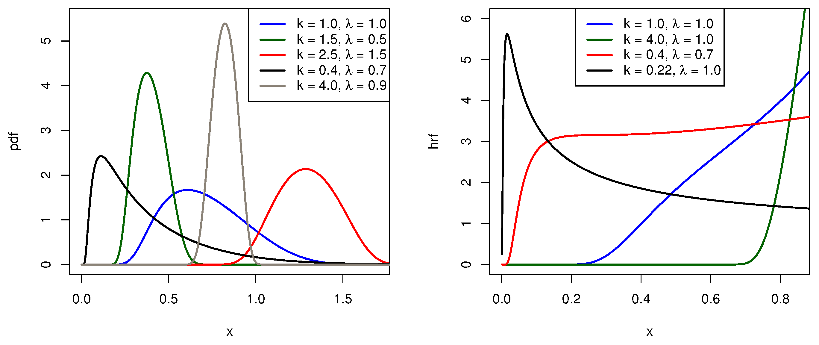
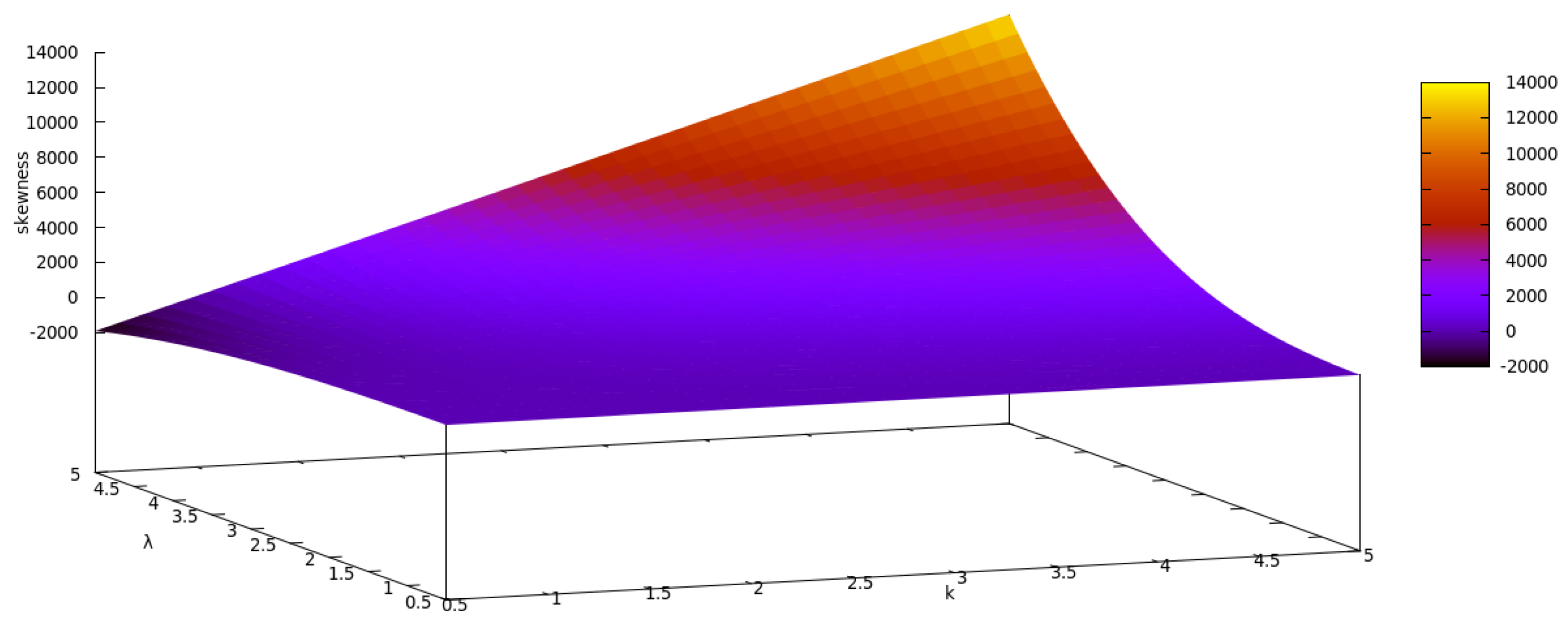
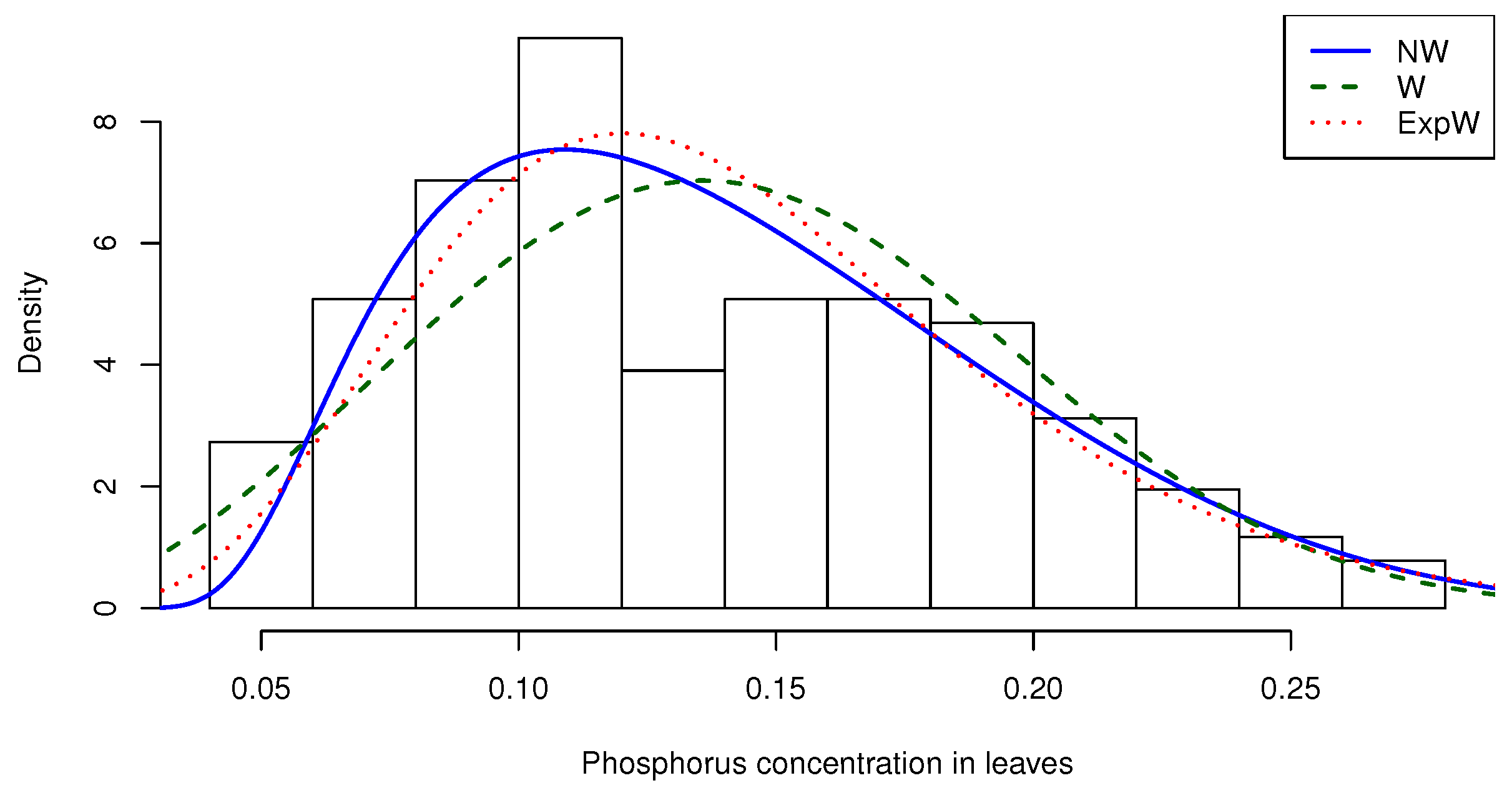
2.1.1. The Normal-Weibull Distribution

Weibull is one of the most used models to describe natural phenomena and failure of several kinds of components. It is extensively used in survival analysis and reliability. In recent times, many authors have focused on new extensions for it, such as [13,14]. The two-parameter Weibull cdf is given by G W ( x | k , λ ) = 1 e ( x / λ ) k for x 0 , where k, λ > 0 . Replacing the baseline G in Equation (4) by G W , we get to the Normal-Weibull cdf, namely:
F N W ( x ) = Φ e ( x / λ ) k 2 1 e ( x / λ ) k ,
for x 0 . Using Equation (5) to write the corresponding pdf, we have:
f N W ( x ) = ϕ e ( x / λ ) k 2 1 e ( x / λ ) k k x k 1 λ k 1 2 1 e ( x / λ ) k e ( x / λ ) k e ( x / λ ) k 1 e ( x / λ ) k 2 .
Plots of pdf and hrf of the Normal-Weibull distribution for different values of the parameters are portrayed in Figure 1. The different shapes of the hrf curve evince the flexibility of the model. Particularly for k = 1 , the Weibull distribution is equivalent to an Exponential distribution, so the hrf is constant; in contrast, the Normal-Exponential model has an increasing hrf in some left-bounded interval.
In Figure 2, the vertical axis shows the range of values of Pearson’s moment coefficient of skewness, which depends on the parameters k and λ . We can see in the graph that the Normal-Weibull distribution is also able to fit data with either positive or negative skew.

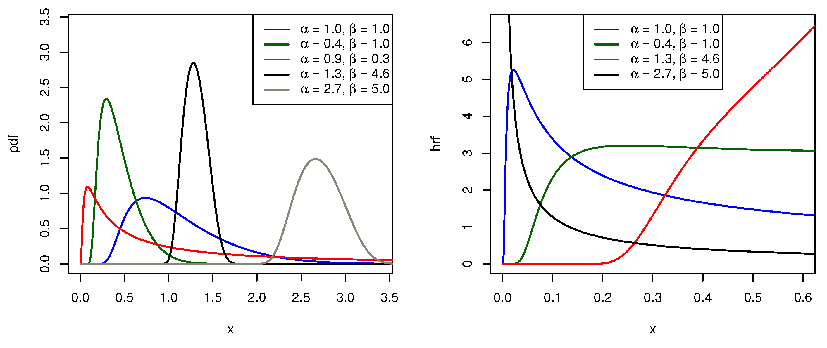
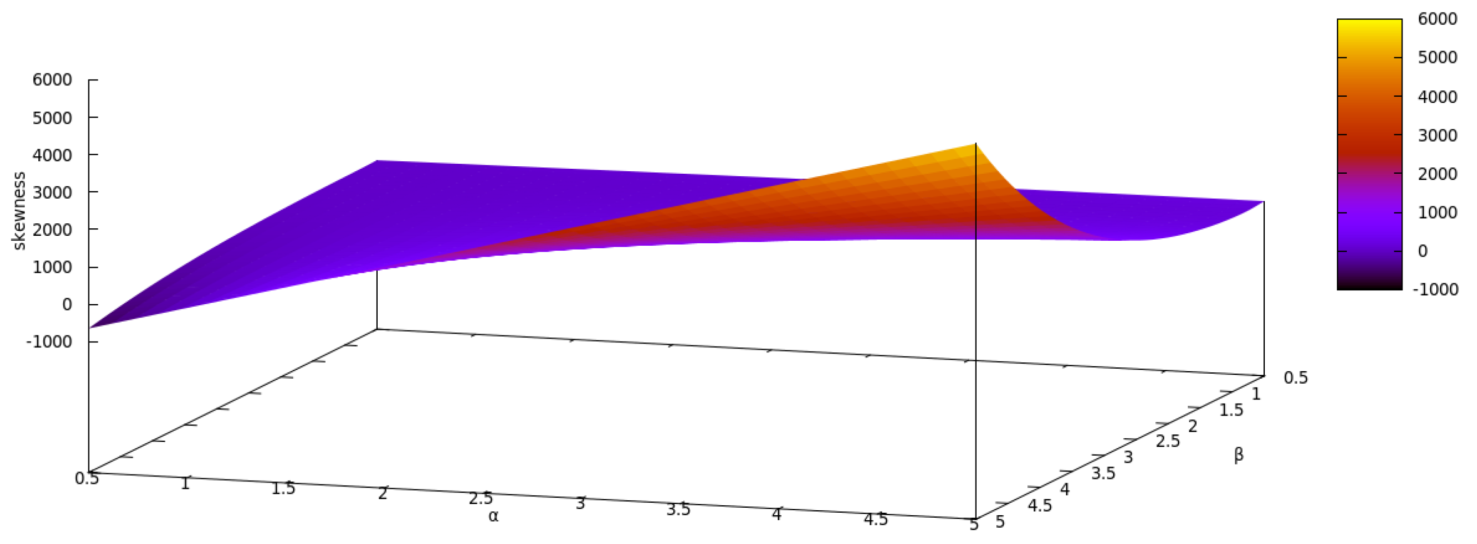
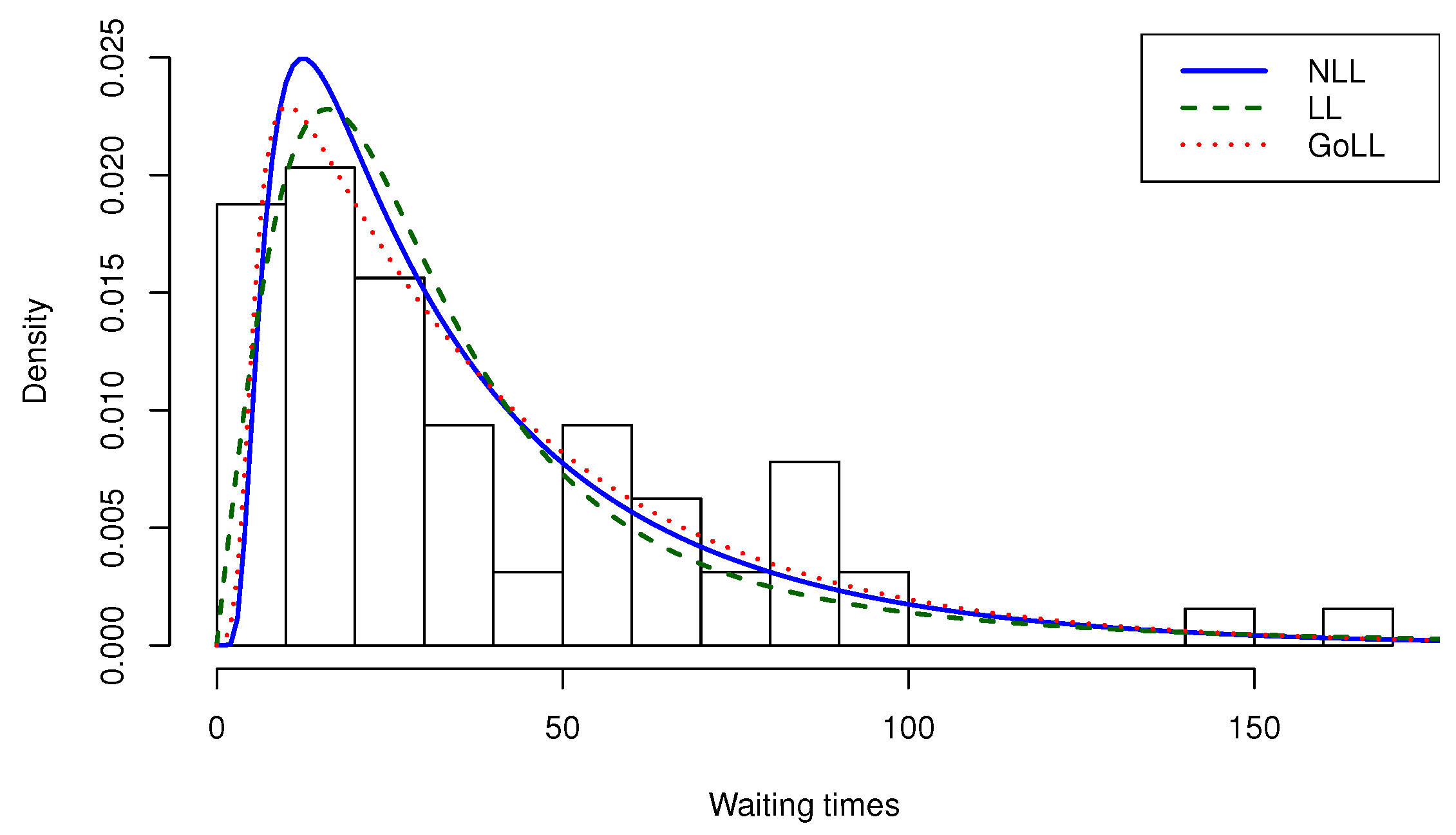
2.1.2. The Normal-Log-Logistic Distribution

The Log-logistic distribution is commonly applied to reliability and oftentimes it works well as a lifetime model. Its cdf is given by G L L ( x | α , β ) = 1 1 + ( x / α ) β 1 for x 0 , where α , β > 0 . The Normal-log-logistic cdf is easily obtained replacing the parent distribution G in Equation (4) by G L L . Thus:
F N L L ( x ) = Φ x α β x α β ,
for x 0 . Taking the derivative of Equation (9) with respect to x, we get to the pdf:
f N L L ( x ) = ϕ x α β x α β 1 + x a 2 β β α β x β 1 .
Figure 3 shows plots of pdf and hrf for different values of α and β . It is worth noting that the Normal-log-logistic distribution may have a decreasing hrf of early failure. It is also possible for the hrf to be increasing or unimodal.
Pearson’s moment coefficient of skewness for the Normal-log-logistic distribution is depicted in Figure 4.

2.2. Series Representation

The normal cdf is related to the error function erf as follows:
Φ ( z ) = 1 2 1 + erf z 2 ,
where erf ( z ) = 2 π 0 z e t 2 d t . Provided that erf ( z / 2 ) can be linearly represented by:
erf z 2 = 2 π n = 0 ( 1 ) n · ( z / 2 ) 2 n + 1 n ! ( 2 n + 1 ) = 2 π · n = 0 1 2 n z 2 n + 1 n ! ( 2 n + 1 ) ,
replacing Equation (12) in Equation (11), we obtain:
Φ ( z ) = 1 2 + 1 2 π n = 0 1 2 n z 2 n + 1 n ! ( 2 n + 1 ) .
Now, considering | G ( x ) | < 1 , we can write:
2 G ( x ) 1 G ( x ) [ 1 G ( x ) ] = 2 G ( x ) 1 G ( x ) · 1 1 G ( x ) = 2 1 G ( x ) k = 0 G ( x ) k
and replacing z of the right member of Equation (13) by the expression in Equation (14), we have:
Φ 2 G ( x ) 1 G ( x ) [ 1 G ( x ) ] = 1 2 + 1 2 π n = 0 ( 1 / 2 ) n n ! ( 2 n + 1 ) 2 1 G ( x ) k = 0 G ( x ) k 2 n + 1 = 1 2 + 1 2 π n = 0 ( 1 / 2 ) n n ! ( 2 n + 1 ) 2 1 G ( x ) 2 n + 1 A 1 k = 0 G ( x ) k 2 n + 1 A 2 .
The right member of Equation (15) has two factors, namely, A1 and A2, that can be rewritten as power series. Concerning to A1, the binomial theorem allows us to write:
2 1 G ( x ) 2 n + 1 = j = 0 2 n + 1 2 n + 1 j 2 2 n + 1 j 1 G ( x ) j = j = 0 2 n + 1 2 n + 1 j ( 1 ) j · 2 2 n + 1 j · G ( x ) j = j = 0 2 n + 1 δ j · G ( x ) j
It is a known result related to power series raised to powers that:
k = 0 a k G ( x ) k N = k = 0 c k G ( x ) k ,
where c 0 = a 0 N , c k = 1 k a 0 s = 1 k ( s N k + s ) a s c k s for k 1 and N N . Setting N = 2 n + 1 and a k = 1 for all k 0 , we get to the expression A2 in Equation (15) and we can use the result in Equation (17) to write as follows:
k = 0 G ( x ) k 2 n + 1 = k = 0 c k · G ( x ) k ,
such that c 0 = 1 , c k = 1 k s = 1 k ( s [ 2 n + 1 ] k + s ) c k s for k 1 and 2 n + 1 N . Now replacing A1 and A2 of the Equation (15) by the right members of the Equations (16) and (18) respectively, we obtain the result below:
Φ 2 G ( x ) 1 G ( x ) [ 1 G ( x ) ] = 1 2 + 1 2 π n = 0 ( 1 / 2 ) n n ! ( 2 n + 1 ) · j = 0 2 n + 1 δ j · G ( x ) j · k = 0 c k · G ( x ) k = 1 2 + n = 0 j = 0 2 n + 1 k = 0 2 n + 1 j ( 1 ) n + j · 2 n + 1 j n ! ( 2 n + 1 ) 2 π c k η j , n , k · G ( x ) k j = 1 2 + n , k = 0 j = 0 2 n + 1 η j , n , k · G ( x ) k j .
The Fubini’s theorem on differentiation allows us to write the derivative of Equation (19) with respect to x as follows:
f G ( x ) = n , k = 0 j = 0 2 n + 1 η j , n , k · ( k j ) g ( x ) G ( x ) k j 1 g k j ( x ) .
Since g k j ( x ) is the pdf of a random variable of the exponentiated family, as described in [15,16], one can say that (20) is the Normal-G pdf (5) expressed as a linear combination of pdfs of exponentiated distributions. Such useful property is typically found and detailed in works on new classes of distributions; see for instance: [17,18,19,20].

2.3. Quantile Function

By inverting Equation (4), the quantile function associated with the Normal-G class is obtained. For simplification, let us write v = F G ( x ) . From Equation (4) we have:
Φ 1 ( v ) = 2 G ( x ) 1 G ( x ) [ 1 G ( x ) ]     Φ 1 ( v ) G ( x ) 2 + [ 2 Φ 1 ( v ) ] G ( x ) 1 = 0 ,
that is, a quadratic equation for G ( x ) , that admits the following two solutions:
Φ 1 ( v ) 2 4 + Φ 1 ( v ) 2 2 Φ 1 ( v )   and   Φ 1 ( v ) 2 + 4 + Φ 1 ( v ) 2 2 Φ 1 ( v ) .
If the first solution above is picked, then G ( x ) might assume values lesser than 0 (see v = 0 . 95 for example). On the other hand, the second one allows us to verify that 0 < G ( x ) < 1 is valid for all x R . Finally, we can write the quantile function of Equation (4) as follows:
Q F ( v ) = Q G Φ 1 ( v ) 2 + 4 + Φ 1 ( v ) 2 2 Φ 1 ( v ) ,
such that Q G ( · ) is the quantile function of the baseline G. A uniform random number generator and (21) make the simulation of random variables following (3) quite simple. Namely, if Z U ( 0 , 1 ) , then  Q F ( Z ) follows a Normal-G distribution.

2.4. Raw Moments, Incomplete Moments and Moment Generating Function

Provided that X follows a Normal-G distribution, the rth raw moment of X is E ( X r ) = x r f G ( x ) d x , where f G ( x ) is given in Equation (20) and r Z + * . Using Fubini’s theorem to change the order of integration and series, we have:
E ( X r ) = n , k = 0 j = 0 2 n + 1 η j , n , k x r g k j ( x ) d x
= n , k = 0 j = 0 2 n + 1 η j , n , k E ( Y k j r )
where Y k j follows the exponentiated distribution whose pdf is g k j ( x ) shown in Equation (20).
Despite the upper infinity limit in the sums, expressions like Equation (23) are not intractable. According to [21], one can get fairly accurate results truncating each infinite sum by 20; they used numerical routines to compute accurately similar expressions for the moments of some Kumaraswamy generalized distributions.
The rth moment can also be represented in terms of the quantile function of the baseline. Defining u = G k j ( x ) and replacing x in Equation (22) by Q G u 1 / ( k j ) , we have:
E ( X r ) = n , k = 0 j = 0 2 n + 1 η j , n , k 0 1 Q G u 1 k j r d u .
The rth incomplete moment of X is given by the following expression:
T r ( z ) = z x r f G ( x ) d x = n , k = 0 j = 0 2 n + 1 η j , n , k T r * ( z )
Where T r * ( z ) is the rth incomplete moment of Y k j . One can also write Equation (24) in terms of the quantile function of G:
T r ( z ) = n , k = 0 j = 0 2 n + 1 η j , n , k 0 [ G ( x ) ] k j Q G u 1 k j r d u .
The mgf is a function associated with a random variable, whose moments can be straightforwardly derived using it. It is also useful to check whether two functions of random variables are equal since there is a bijection between pdfs and mgfs (when they exist). The mgf M X ( t ) of X is the expected value of e t X , where t ( ι , ι ) , ι > 0 . Given that M Y k j ( t ) is the mgf of Y k j , on the lines of Equation (23), we can write:
M X ( t ) = n , k = 0 j = 0 2 n + 1 η j , n , k e t x g k j ( x ) d x = n , k = 0 j = 0 2 n + 1 η j , n , k M Y k j ( t ) .

2.5. Estimation and Inference

Attractive asymptotic properties, such as efficiency and consistency, are some of the reasons that make the maximum likelihood method the most usually applied method of parametric point estimation. The MLEs are the points that maximize the likelihood function over the domain of the parameter space. Since the logarithmic function is increasing, performing the maximization of the log-likelihood function, besides being a more convenient task, also provides the MLEs.
Given that ξ = ( ξ 1 , , ξ r ) is the r × 1 parametric vector of a random variable X that follows a Normal-G distribution, G ( x | ξ ) = G ξ ( x ) is the baseline, g ( x | ξ ) = g ξ ( x ) is its corresponding pdf and X = ( x 1 , , x m ) is a complete random sample of size m from X, then the log-likelihood function is:
( ξ | X ) = j = 1 m log ϕ 2 G ξ ( x j ) 1 G ξ ( x j ) 1 G ξ ( x j ) + j = 1 m log 1 2 G ξ ( x j ) + 2 G ξ 2 ( x j ) 2 j = 1 m log G ξ ( x j ) 2 j = 1 m log 1 G ξ ( x j ) + j = 1 m log g ξ ( x j ) .
Thanks to powerful functions available within the software for statistical computing, it is possible to use numerical methods to maximize (25); for this purpose, R [22] brings the function optim in package stats.
The MLEs can also be obtained by solving the system of equations U ( ξ | X ) = 0 r , where U ( ξ | X ) = ξ ( ξ | X ) = ( u i ) 1 i r is the score vector, such that:
u i = j = 1 m [ G ξ ( x j ) 1 ] 4 G ξ 4 ( x j ) G ξ 3 ( x j ) [ 1 G ξ ( x j ) ] 3 · ξ i G ξ ( x j ) + j = 1 m 4 G ξ ( x j ) 2 1 2 G ξ ( x j ) + 2 G ξ 2 ( x j ) · ξ i G ξ ( x j ) 2 j = 1 m 1 G ξ ( x j ) · ξ i G ξ ( x j ) + 2 j = 1 m 1 1 G ξ ( x j ) · ξ i G ξ ( x j ) + j = 1 m 1 g ξ ( x j ) · ξ i g ξ ( x j )
and 0 r is a r × 1 vector of zeros.
The information matrix J ( ξ | X ) is essential to construct confidence intervals and to test hypotheses on ξ . The expectation of J ( ξ | X ) is the expected Fisher information matrix I ξ and under certain conditions of regularity, m ( ξ ^ ξ ) follows approximately a multivariate normal distribution N r 0 r , I ξ 1 . The expression for J ( ξ | X ) is presented in Appendix A.

3. Numerical Analysis

3.1. Simulation Study

We used the free software R version 3.4.4 [22] to carry out the Monte Carlo simulation study; the number of replications was 10,000. The pseudo-random samples were generated via Von Neumann’s acceptance-rejection method [23]. This simple procedure requires the corresponding pdf y = f ( x ) , a minorant and a majorant for x and a majorant for y; it is not necessary to implement the quantile function in this case. Four sample sizes, namely n = 50 , 100, 200 and 500, and five different values for the vector of parameters were considered. For each scenario, we calculated the bias and the mean squared error (MSE) as follows:
Bias i = 1 10000 j = 1 10000 ξ ^ i j ξ i ,   MSE i = 1 10000 j = 1 10000 ξ ^ i j ξ i 2
where ξ i is the i-th element of the vector of parameters ξ = ( ξ 1 , , ξ r ) and ξ ^ i j is the estimate for ξ i at the j-th replication. The log-likelihood function was maximized using the technique of simulated annealing, available by the optim subroutine, for which the user has to pass a vector ξ 0 of initial values. At first, we took ξ 0 = 1 r , namely a r × 1 vector of ones, then we run one single replication considering sample size n = 50 ; the obtained estimates from this procedure were assigned to ξ 0 and used in all of the aforementioned scenarios.
The results for both parameters of the Normal-Weibull density (8), shown in Table 1, indicate that the estimates are fairly close to the actual values. Moreover, as it would be expected, the bigger the sample size, the smaller the MSEs.
The results given in Table 2 suggest that the estimates of the parameters of the Normal-log-logistic model (10) have similar behavior of those shown in Table 1, that is to say, the biases are quite small and the MSE decreases as the sample size increases.

3.2. Applications

The first data to be considered is related to the soil fertility influence and the characterization of the biologic fixation of N2 for the Dimorphandra wilsonii Rizz growth. It was originally studied by [24] and it also figures in the work of [25]. For 128 plants, the phosphorus concentration in the leaves was quantified. Here are the numbers: 0.22, 0.17, 0.11, 0.10, 0.15, 0.06, 0.05, 0.07, 0.12, 0.09, 0.23, 0.25, 0.23, 0.24, 0.20, 0.08, 0.11, 0.12, 0.10, 0.06, 0.20, 0.17, 0.20, 0.11, 0.16, 0.09, 0.10, 0.12, 0.12, 0.10, 0.09, 0.17, 0.19, 0.21, 0.18, 0.26, 0.19, 0.17, 0.18, 0.20, 0.24, 0.19, 0.21, 0.22, 0.17, 0.08, 0.08, 0.06, 0.09, 0.22, 0.23, 0.22, 0.19, 0.27, 0.16, 0.28, 0.11, 0.10, 0.20, 0.12, 0.15, 0.08, 0.12, 0.09, 0.14, 0.07, 0.09, 0.05, 0.06, 0.11, 0.16, 0.20, 0.25, 0.16, 0.13, 0.11, 0.11, 0.11, 0.08, 0.22, 0.11, 0.13, 0.12, 0.15, 0.12, 0.11, 0.11, 0.15, 0.10, 0.15, 0.17, 0.14, 0.12, 0.18, 0.14, 0.18, 0.13, 0.12, 0.14, 0.09, 0.10, 0.13, 0.09, 0.11, 0.11, 0.14, 0.07, 0.07, 0.19, 0.17, 0.18, 0.16, 0.19, 0.15, 0.07, 0.09, 0.17, 0.10, 0.08, 0.15, 0.21, 0.16, 0.08, 0.10, 0.06, 0.08, 0.12, 0.13. Table 3 brings some descriptive statistics.
We fitted the Normal-Weibull distribution (NW) (7) to the soil fertility dataset and compared it to the fits of Weibull (W), Exponentiated Weibull (ExpW) [1], Marshall-Olkin Extended Weibull (MOEW) [26], Kumaraswamy-Weibull (KwW) [9], Beta-Weibull (BW) [8] and McDonald-Weibull (McW) [7]. The function goodness.fit of the R package AdequacyModel provides, besides the MLEs and the standard errors (SE), some criteria for model selection (AIC, CAIC, BIC and HQIC); they are shown in Table 4.
Information criteria may be used as relative goodness-of-fit measures, such that the lowest values will characterize the best fitted models. In this sense, the Normal-Weibull distribution outperforms the other ones.
Figure 5 shows the histogram of soil fertility data and the fitted densities with the three lowest values of AIC among the distributions in the first column of Table 4. Although the Normal-Weibull and Exponentiated Weibull curves appear to be very close, the blue one (NW) seems to be closer to the histogram.
The modified versions of Anderson-Darling ( A * ) and Cramér-von Mises ( W * ) statistics (more details in [27]) are typically used to investigate the quality of fit of probabilistic models. Table 5 brings these statistics concerning the fitted models to soil fertility data.
The measures portrayed in Table 5 represent the difference between the empirical distribution function and the real underlying cdf; hence we will consider that the models with lower values of A * and W * fit the data better. Therefore, once again the Normal-Weibull distribution beats the competing models.
The second application concerns to a dataset representing waiting times (in seconds) between 65 successive eruptions of water through a hole in the cliff at the coastal town of Kiama (New South Wales, Australia), known as the Blowhole. These data can be obtained in [17,28]. Here are they: 83, 51, 87, 60, 28, 95, 8, 27, 15, 10, 18, 16, 29, 54, 91, 8, 17, 55, 10, 35,47, 77, 36, 17, 21, 36, 18, 40, 10, 7, 34, 27, 28, 56, 8, 25, 68, 146, 89, 18, 73, 69, 9, 37, 10, 82, 29, 8, 60, 61, 61, 18, 169, 25, 8, 26, 11, 83, 11, 42, 17, 14, 9, 12. Table 6 provides descriptive statistics.
We fitted the Normal-log-logistic distribution (NLL) (9) to the eruption dataset and compared it to the fits of Log-logistic (LL), Exponentiated Log-logistic (ExpLL), Beta-log-logistic (BLL), Kumaraswamy-log-logistic (KwLL) and Gompertz-log-logistic (GoLL); the four latter along the lines of [1,8,9,11] respectively. Table 7 brings the MLEs, SEs and information criteria.
Since the Normal-log-logistic fitted model presents the smallest values of AIC, CAIC, BIC and HQIC compared to the fits of the other distributions, selecting it rather than the others is a reasonable decision in this case.
In Figure 6 the histogram of eruption data and the fitted densities with the three lowest values of AIC among the distributions in the first column of Table 7 are depicted. By a visual comparison, the three curves are apparently good approximations to the histogram, but the Normal-log-logistic’s seems to explain the behavior of the data more accurately.
Table 8 provides the values of A * and W * of the distributions in the first column of Table 7. These statistics suggest that GoLL and NLL models fit the eruption dataset very closely. Nonetheless, in order to pick a more parsimonious model, one should prefer the NLL, since it has fewer parameters than GoLL.
It is worth mentioning that [17] proposed the new class Exponentiated Kumaraswamy-G and fitted one of its submodels (with Weibull as baseline) to the same eruption dataset. It presented A * = 0 . 7594 and W * = 0 . 1037 , whereas NLL presented lower values of these statistics as one can check in Table 8.

4. Concluding Remarks

Based on the method of generating classes of probability distributions presented by [12], we introduce a new class called Normal-G. It has the advantage of demanding no additional parameters besides the baseline ones. We demonstrate that the proposed class generates identifiable sub-models as long as the parent distribution is identifiable. The pdf of the class can be written as a linear combination of pdfs of exponentiated distributions; it allows us to easily derive the raw moments, the incomplete moments and the moment generating function.
We bring Monte Carlo simulation studies to attest the good performance of the MLEs of two distributions generated by the class and to illustrate its usefulness, applications to real datasets are made. The fitted models are compared to other competitive distributions regarding the Anderson-Darling and the Cramér-von Mises statistics, as well as commonly used information criteria as goodness-of-fit measures. The general results indicate that the Normal-G outperforms the other distributions in comparison. The new class is powerful and provides parsimonious models, which may hopefully interest practitioners of statistics, soil science, oceanography and other fields.

Author Contributions

All of the authors contributed relevantly to this research article.

Funding

This research received no external funding.

Conflicts of Interest

The authors declare no conflict of interest.

Appendix A

The information matrix mentioned in Section 2.5 is given by
J ( ξ | X ) = ξ ξ ( ξ | X ) = ( u i h ) 1 i r , 1 h r , where:
u i h = j = 1 m 2 G ξ ( x j ) 3 G ξ 4 ( x j ) 2 G ξ ( x j ) + 1 [ 1 G ξ ( x j ) ] 4 · ξ i G ξ ( x j ) · ξ h G ξ ( x j ) + j = 1 m [ 1 G ξ ( x j ) ] 4 G ξ 4 ( x j ) G ξ 3 ( x j ) [ 1 G ξ ( x j ) ] 3 · 2 ξ i ξ h G ξ ( x j ) + j = 1 m 8 [ 1 G ξ ( x j ) ] G ξ ( x j ) 1 2 G ξ ( x j ) + 2 G ξ 2 ( x j ) · ξ i G ξ ( x j ) · ξ h G ξ ( x j ) + j = 1 m 4 G ξ ( x j ) 2 1 2 G ξ ( x j ) + 2 G ξ 2 ( x j ) · 2 ξ i ξ h G ξ ( x j ) + j = 1 m 2 G ξ 2 ( x j ) · ξ i G ξ ( x j ) · ξ h G ξ ( x j ) j = 1 m 2 G ξ ( x j ) · 2 ξ i ξ h G ξ ( x j ) + j = 1 m 2 [ 1 G ξ ( x j ) ] 2 · ξ i G ξ ( x j ) · ξ h G ξ ( x j ) + j = 1 m 2 1 G ξ ( x j ) · 2 ξ i ξ h G ξ ( x j ) j = 1 m 1 g ξ 2 ( x j ) · ξ i g ξ ( x j ) · ξ h g ξ ( x j ) + j = 1 m 1 g ξ ( x j ) · 2 ξ i ξ h g ξ ( x j ) .

References

  1. Mudholkar, G.S.; Srivastava, D.K.; Freimer, M. The exponentiated Weibull family: A reanalysis of the bus motor failure data. Technometrics 1995, 37, 436–445. [Google Scholar] [CrossRef]
  2. Gupta, R.D.; Kundu, D. Generalized Exponential Distributions. Aust. N. Z. J. Stat. 1999, 41, 173–188. [Google Scholar] [CrossRef]
  3. Marshall, A.W.; Olkin, I. A new method for adding a parameter to a family of distributions with application to the exponential and Weibull families. Biometrika 1997, 84, 641–652. [Google Scholar] [CrossRef]
  4. Nadarajah, S. A Generalized Normal Distribution. J. Appl. Stat. 2005, 32, 685–694. [Google Scholar] [CrossRef]
  5. Azzalini, A. A Class of Distributions which includes the Normal ones. Scand. J. Stat. 1985, 12, 171–178. [Google Scholar]
  6. Robertson, H.T.; Allison, D.B. A Novel Generalized Normal Distribution for Human Longevity and other Negatively Skewed Data. PLoS ONE 2012, 7, e37025. [Google Scholar] [CrossRef]
  7. Cordeiro, G.M.; Hashimoto, E.M.; Ortega, E.M.M. The McDonald Weibull Model. Statistics 2014, 48, 256–278. [Google Scholar] [CrossRef]
  8. Famoye, F.; Lee, C.; Olumolade, O. The Beta-Weibull distribution. J. Stat. Theory Appl. 2005, 4, 121–136. [Google Scholar]
  9. Cordeiro, G.M.; Castro, M. A new family of generalized distributions. J. Stat. Comput. Simul. 2010, 81, 883–898. [Google Scholar] [CrossRef]
  10. Alzaatreh, A.; Lee, C.; Famoye, F. A new method for generating families of continuous distributions. Metron 2013, 71, 63–79. [Google Scholar] [CrossRef]
  11. Alizadeh, M.; Cordeiro, G.M.; Pinho, L.G.B.; Ghosh, I. The Gompertz-G family of distributions. J. Stat. Theory Pract. 2017, 11, 179–207. [Google Scholar] [CrossRef]
  12. Brito, C.R.; Rêgo, L.C.; Oliveira, W.R.; Gomes-Silva, F. Method for Generating Distributions and Classes of Probability Distributions: The Univariate Case. Hacet. J. Math. Stat. 2019, 48, 897–930. [Google Scholar]
  13. Xie, M.; Tang, Y.; Goh, T.N. A modified Weibull extension with bathtub-shaped failure rate function. Reliab. Eng. Syst. Safe. 2002, 76, 279–285. [Google Scholar] [CrossRef]
  14. Bebbington, M.; Lai, C.D.; Zitikis, R. A flexible Weibull extension. Reliab. Eng. Syst. Safe. 2007, 92, 719–726. [Google Scholar] [CrossRef]
  15. Tahir, M.H.; Nadarajah, S. Parameter induction in continuous univariate distributions: Well-established G families. An. Acad. Bras. Ciênc. 2015, 87, 539–568. [Google Scholar] [CrossRef]
  16. Cordeiro, G.M.; Ortega, E.M.M.; Cunha, D.C.C. The Exponentiated Generalized Class of Distributions. J. Data Sci. 2013, 11, 1–27. [Google Scholar]
  17. Silva, R.; Gomes-Silva, F.; Ramos, M.; Cordeiro, G.; Marinho, P.; Andrade, T.A.N. The Exponentiated Kumaraswamy-G Class: General Properties and Application. Rev. Colomb. Estad. 2019, 42, 1–33. [Google Scholar] [CrossRef]
  18. Cakmakyapan, S.; Ozel, G. The Lindley Family of Distributions: Properties and Applications. Hacet. J. Math. Stat. 2017, 46, 1113–1137. [Google Scholar] [CrossRef]
  19. Barreto-Souza, W.; Cordeiro, G.M.; Simas, A.B. Some Results for Beta Fréchet Distribution. Commun. Stat. Theory Methods 2011, 40, 798–811. [Google Scholar] [CrossRef]
  20. Huang, S.; Oluyede, B.O. Exponentiated Kumaraswamy-Dagum distribution with applications to income and lifetime data. J. Stat. Dist. Appl. 2014, 1, 1–20. [Google Scholar] [CrossRef]
  21. Cordeiro, G.M.; Bager, R.S.B. Moments for Some Kumaraswamy Generalized Distributions. Comm. Statist. Theory Methods 2015, 44, 2720–2737. [Google Scholar] [CrossRef]
  22. R Core Team. R: A Language and Environment for Statistical Computing; R Foundation for Statistical Computing: Vienna, Austria, 2018. [Google Scholar]
  23. Von Neumann, J. Various techniques used in connection with random digits. In Applied Mathematics Series 12; National Bureau of Standards: Washington, DC, USA, 1951; pp. 36–38. [Google Scholar]
  24. Fonseca, M.B. A influência da fertilidade do solo e caracterização da fixação biológica de N2 para o crescimento de Dimorphandra wilsonii Rizz. Master’s Thesis, Federal University of Minas Gerais, Belo Horizonte, Brazil, 2007. [Google Scholar]
  25. Silva, R.B.; Bourguignon, M.; Dias, C.R.B.; Cordeiro, G.M. The compound class of extended Weibull power series distributions. Comput. Stat. Data Anal. 2013, 58, 352–367. [Google Scholar] [CrossRef]
  26. Cordeiro, G.M.; Lemonte, A.J. On the Marshall–Olkin extended Weibull distribution. Stat. Pap. 2013, 54, 333–353. [Google Scholar] [CrossRef]
  27. Chen, G.; Balakrishnan, N. A general purpose approximate goodness-of-fit test. J. Qual. Technol. 1995, 27, 154–161. [Google Scholar] [CrossRef]
  28. StatSci.org. Available online: http://www.statsci.org/data/oz/kiama.html (accessed on 21 October 2019).
Figure 1. Plots of pdf and hrf for the Normal-Weibull distribution.
Symmetry 11 01407 g001
Figure 2. Skewness of the Normal-Weibull distribution.
Symmetry 11 01407 g002
Figure 3. Plots of pdf and hrf for the Normal-log-logistic distribution.
Symmetry 11 01407 g003
Figure 4. Skewness of the Normal-log-logistic distribution.
Symmetry 11 01407 g004
Figure 5. Histogram of soil fertility dataset and fitted densities.
Symmetry 11 01407 g005
Figure 6. Histogram of eruption dataset and fitted densities.
Symmetry 11 01407 g006
Table 1. Bias and MSE of the estimates under the maximum likelihood method for the Normal-Weibull model.
Actual ValueBiasMSE
n k λ k ^ λ ^ k ^ λ ^
501.01.70.02707850−0.009481100.008222990.00659991
0.52.00.01446186−0.020371250.002090510.03647395
3.00.50.07878343−0.000967780.073526250.00006357
0.94.00.02586182−0.027521010.006754520.04497248
7.15.80.19086399−0.005404070.414021780.00153179
1001.01.70.01306919−0.004539810.003778830.00332042
0.52.00.00726917−0.014123730.000957860.01838681
3.00.50.03914672−0.000577660.034009290.00003204
0.94.00.01167774−0.014032190.003059030.02273089
7.15.80.08363335−0.002794510.188358560.00077190
2001.01.70.00651588−0.002538200.001814090.00166703
0.52.00.00358578−0.006781780.000456810.00923355
3.00.50.01901041−0.000293620.016286770.00001604
0.94.00.00658567−0.007455410.001480590.01138373
7.15.80.03656102−0.000663160.090416100.00038519
5001.01.70.00317837−0.001272340.000711640.00066754
0.52.00.00195165−0.006098000.000179670.00370983
3.00.50.00748033−0.000088040.006360080.00000641
0.94.00.00297109−0.002005330.000577440.00455810
7.15.80.01427116−0.000458890.035500630.00015444
Table 2. Bias and MSE of the estimates under the maximum likelihood method for the Normal-log-logistic model.
Actual ValueBiasMSE
n α β α ^ β ^ α ^ β ^
502.75.00.000544040.134247000.001095510.20695579
0.41.20.000245670.032758570.000418640.01195999
6.02.5−0.000021680.068353250.021618470.05192641
4.03.40.001856590.089971530.005212510.09539035
1.08.00.000101810.218358540.000058680.53164800
1002.75.00.000120460.063770310.000556940.09509012
0.41.20.000051010.015190260.000212460.00547655
6.02.50.001917690.032978880.010998440.02386620
4.03.4−0.000049230.047011710.002638200.04439236
1.08.00.000098270.110574190.000029800.24582360
2002.75.00.000155040.032992120.000280470.04585339
0.41.20.000065510.008665070.000106770.00265802
6.02.5−0.001062770.016253140.005538910.01145699
4.03.4−0.000024070.022955670.001330640.02123514
1.08.00.000008520.050909230.000015030.11715066
5002.75.00.000215580.013274690.000112770.01789692
0.41.2−0.000089410.004356330.000042840.00104215
6.02.5−0.000423580.006482520.002226390.00447192
4.03.4−0.000077890.008556090.000535130.00826466
1.08.00.000039540.016637110.000006040.04559331
Table 3. Descriptive statistics for soil fertility dataset.
nmeanmedianminmaxVarianceSkewnessKurtosis
1280.140780.130.050.280.002960.45438−0.64478
Table 4. Fitted distributions to the soil fertility dataset (estimates and information criteria).
DistributionParametersEstimates (SE)AICCAICBICHQIC
NWk0.8398477 (0.0445182) 395 . 7584 395 . 6624 390 . 0544 393 . 4408
λ 0.2049909 (0.0074017)
Wk2.8185566 (0.1919639) 385 . 6297 385 . 5337 379 . 9256 383 . 3121
λ 0.1584836 (0.0052564)
ExpWk1.5321145 (0.5023377) 387 . 4361 387 . 2426 378 . 8801 383 . 9598
λ 0.0939938 (0.0374090)
a3.5076974 (2.6763009)
MOEWk3.9300962 (0.2426080) 377 . 9475 377 . 754 369 . 3914 374 . 4711
λ 8.9163819 (4.5940983)
a0.0031628 (0.0007240)
KwWk1.1503912 (0.3443931) 384 . 1491 383 . 8239 372 . 7409 379 . 5139
λ 0.1953371 (0.1291154)
a3.3444607 (1.5352029)
b7.5480698 (10.206142)
BWk0.8477957 (0.2166409) 385 . 7589 385 . 4337 374 . 3508 381 . 1237
λ 0.3304922 (0.4395169)
a9.0436364 (4.5271059)
b15.211970 (22.481984)
McWk5.6665646 (8.3928707) 384 . 6657 384 . 1739 370 . 4055 378 . 8717
λ 0.5912941 (0.5124852)
a13.441193 (23.051917)
b14.363802 (18.264058)
c0.0870787 (0.1234075)
Table 5. Goodness-of-fit test statistics.
Distribution A * W *
NW0.4540080.079841
W1.1569940.207118
ExpW0.7844510.138403
MOEW1.1237590.183128
KwW0.9072390.163617
BW0.7505930.130501
McW0.7582960.137509
Table 6. Descriptive statistics for eruption dataset.
nMeanMedianminmaxVarianceSkewnessKurtosis
6439.828122871691139.0971.546412.77108
Table 7. Fitted distributions to the eruption dataset (estimates and information criteria).
DistributionParametersEstimates (SE)AICCAICBICHQIC
NLL α 28.71747 (2.751091)587.5681587.7649591.8859589.2691
β 0.568200 (0.042998)
LL α 28.27831 (3.203986)597.1497597.3464601.4674598.8506
β 1.969345 (0.198878)
ExpLL α 7.394859 (6.479904)597.3629597.7629603.8396599.9144
β 1.461528 (0.197256)
a4.572569 (4.470086)
BLL α 7.445103 (10.72863)596.186596.864604.8215599.588
β 0.484528 (0.223626)
a17.28664 (13.82502)
b9.285354 (9.566756)
KwLL α 2.107772 (5.325557)596.68597.358605.3156600.082
β 0.511324 (0.130629)
a12.14489 (12.25210)
b11.42477 (8.749787)
GoLL α 5.667167 (1.680598)591.7172592.3952600.3528595.1192
β 4.348435 (1.450980)
a0.035617 (0.017111)
b0.234894 (0.100666)
Table 8. Goodness-of-fit tests.
Distribution A * W *
NLL0.6122910.0803799
LL1.0191290.1413872
ExpLL1.1382180.1617136
BLL0.8372110.1141264
KwLL0.8180720.1118931
GoLL0.6058220.0805111

