Study of Indoor Ventilation Based on Large-Scale DNS by a Domain Decomposition Method

1
School of Aeronautics and Astronautics, Sun Yat-Sen University, Guangzhou 510275, China
2
Department of Thermal Science and Energy Engineering, University of Science and Technology of China, Hefei 230027, China
3
Department of Mechanical Engineering, the University of Hong Kong, Hong Kong 999077, China
*
Author to whom correspondence should be addressed.
Symmetry 2019, 11(11), 1416; https://0-doi-org.brum.beds.ac.uk/10.3390/sym11111416
Submission received: 15 October 2019
/
Revised: 6 November 2019
/
Accepted: 8 November 2019
/
Published: 15 November 2019
(This article belongs to the Special Issue Mathematical Modeling and Computational Methods in Science and Engineering)
Abstract
:This paper presents a large-scale Domain Decomposition Method (DDM) based Direct Numerical Simulation (DNS) for predicting the behavior of indoor airflow, where the aim is to design a comfortable and efficient indoor air environment of modern buildings. An analogy of the single-phase convection problems is applied, and the pressure stabilized domain decomposition method is used to symmetrize the linear systems of Navier-Stokes equations and the convection-diffusion equation. Furthermore, a balancing preconditioned conjugate gradient method is utilized to deal with the interface problem caused by domain decomposition. The entire simulation model is validated by comparing the numerical results with that of recognized experimental and numerical data from previous literature. The transient behavior of indoor airflow and its complexity in the ventilated room are discussed; the velocity and vortex distribution of airflow are investigated, and its possible influence on particle accumulation is classified.
1. Introduction
The Heating, Ventilation and Air Conditioning (HVAC) system has become the primary mechanism for maintaining the acceptable indoor air quality in modern buildings. Thus, the proper design of HVAC systems is strongly connected to physical health [1,2,3,4,5]. However, one problem associated with HVAC systems is that, in a typical working environment involving the emission of gases or dust, it is necessary to select a high enough ventilation flow rate to remove the generated air contaminants such as [6,7,8]. However, the ventilation rate also implies increasing the ventilated heat from the indoor environment, which of course reduces the building’s energy management efficiency [9,10,11]. One solution to this problem is the efficiency improvement of ventilation systems, minimizing the required increases in ventilation rates and energy consumption. In this case, efficiency means that the properly conditioned ventilation air is effectively delivered to indoor space instead of individually to the mechanical performance of the ventilation system. In order to analyze the efficiency of air delivery, the connections between geometric room parameters and the airflow patterns they produce need to be determined [6,9,12,13].
According to many researchers, computational fluid dynamics (CFD) of the flow field and pollutant transport is becoming more and more valuable for assessing indoor ventilation designs [14,15,16]. Furthermore, due to ongoing developments for maximizing the computational power of computers, numerical simulations for indoor airflow prediction are becoming more commonly employed for the design process [11,17,18]. There are several investigations conducted under the condition of idealized indoor space, especially involving rooms with complex structures, by researchers like Yudison [19], Lu [11], Kao [20], Loannis [15], Chung [10]. During the design process, many complex elements must be considered, e.g. modeling the complex geometries, which may lead to a flow field that involves turbulence, recirculation, flow separation and buoyancy [6]. Based on the conclusion drew by Guerra, all present turbulence models fail to accurately represent three-dimensional (3D) boundary layers, especially the separation boundary layers [21]. Moreover, existing turbulence models are developed based on the assumption of involving a high Reynolds number, which is inadequate for low-speed airflows as typically encountered in modern buildings [18,22,23,24].
The ability of simulations to demonstrate the effect of obstructions on airflow is another critical problem that must be considered. Large streamline curvatures are commonly caused by the presence of massive objects, which may lead to strains that simple turbulence models cannot correctly represent. Furthermore, all numerical models need to be validated by experimental data, but the dearth of this kind of data has impeded the further study of even slightly complicated indoor air flows [16,25].
In order to assist the exploration of potential application of DNS methods based on DDM on indoor air ventilation design, this paper compares our DNS results with previous studies from [6], including the 3D Computational Fluid Dynamics (CFD) results with Laser Doppler Anemometry (LDA) data, Particle Imagine Velocimetry (PIV) measurements of airflow in an isothermal model room as well as other forms of simulation results [26]. Since the real situation in indoor spaces is complicated as a result of the problems such as moving boundaries and temperature gradients, the primary purpose of this study is to evaluate the effectiveness of the DNS by a domain decomposition method (DDM) in capturing the detailed flow near substantial flow obstruction.
Indoor airflows are usually characterized by low-Reynolds number (LRN) turbulence. Turbulent flow, the dominant flow pattern in indoor airflow, is mainly solved by three methods: Direct Numerical Simulation (DNS), Large Eddy Simulation (LES) and Reynolds-averaged Navier-Stokes (RANS) [22,23,24,27]. LES and RANS are more reliable under the condition of high Reynolds number. DNS provides the most accurate description of indoor airflow. Meanwhile, researchers have also attempted to adopt other models, such as [28]. Utilizing the open-source computational platform ADVENTURE, a DNS solver based on DDM for a large-scale simulation is developed in this work, and an indoor ventilation model is numerically simulated. In this method, the linear systems of Navier-Stokes equations and the convection-diffusion equation has been symmetrized with a pressure stabilized DDM. Moreover, a balancing preconditioned conjugate gradient method is utilized to solve the interface problem caused by domain decomposition. The research process includes model construction, boundary conditions setting, mesh division, numerical computation and analysis of the results. Based on the results obtained from the simulation, it is reasonable to demonstrate that the numerical results agree with the collected experimental data. According to comparison, DNS based on DDM is more accurate and reliable than model, large eddy simulation and . Therefore, large scale simulation with DNS based on DDM is a relatively accurate way to estimate the indoor airflow behavior, which could be an assistant to a better ventilation environment management.
This paper is arranged as follows: Section 2 gives a brief description of the governing equations in the numerical model and the domain decomposition method (DDM). Section 3 gives the parallel efficiency of the present scheme, the model structure and its parameter settings. Numerical results and its analysis are presented in Section 4 and conclusions are drawn in Section 5.
2. Methods
2.1. Governing Equations
For a three-dimensional domain polyhedral domain , let be the boundary. The parameter is the first-order Sobolev space and is the space of square-summable functions on Under the assumption that the flow field is incompressible and viscous, the model is solved by finding a combination of in space , such that for any , the following set of equations [29] hold:
where is the material derivative operator; is the velocity vector [m/s]; is the density [kg/m3]; is the gravity force[m/s2]; is the dimensionless concentration expansion coefficient; and is the mass concentration and reference mass concentration, respectively; is the diffusion coefficient [m2/s] and is the source term [1/s]; is the stress tensor [N/m2] defined as:
With the Kronecker delta and the viscosity [kg/ms]; is the relative pressure [Pa] (reference pressure equals 101.325 kPa). Initial velocity is applied in at Dirichlet boundary conditions are
and the Neumann boundary conditions are given as:
where and is the outward normal direction to An initial concentration is applied in at and the Dirichlet and Neumann boundary conditions are shown as follows:
where , is the outward normal vector to
2.2. Characteristic Finite Element Scheme
The equations are linearized by using a characteristic finite element scheme [30], where the material derivative in Equation (1) at the nth time step is denoted as
where stands for and in Equation (1) respectively, and the so-called characteristic curve of is a solution of the ordinary differential equation:
With the 1st-order approximation , the material derivative operator can be linearized as follow:
Let denote a triangulation of consisting of tetrahedral elements, where the subscript denotes the representative length of the triangulation. The notations for finite element spaces are as follows:
Note that piecewise linear interpolations are employed for both velocity and pressure, which does not satisfy the “inf-sup” condition, as proposed in [31]; therefore, to enhance the link between velocity and pressure space, a stabilization method for the saddle point problem [32] is utilized in this work, and the finite element scheme for the flow field in Equation (1) reads as follows:
Finding such that
Let defines the inner product, then the continuous bilinear forms and in Equation (10) are introduced as:
where , and
respectively. The stabilization parameter:
where denotes the maximum diameter of an element , and is the infinity norm. Similarly, the finite element scheme for the concentration convection component of Equation (1) finds , such that:
A weak coupling of Finite Element scheme of Equation (10) and Equation (14) is applied in practice; the element searching algorithm for the Lagrange-Galerkin method only needs to be implemented once in a non-steady loop [11].
2.3. Domain Decomposition Method
The finite element discretization of governing equations yields a linear system of the form:
where is the global stiffness matrix, is the unknown vector, which consists of velocity, pressure and concentration at each node. and is the known vector from the reshaped Equation (10) and Equation (14) By the domain decomposition method (DDM), is decomposed into non-overlapping subdomains and the substructuring is performed as follows [33]:
where is the local stiffness matrix corresponding to a subdomain, is the mapping matrix which translates the global indices of the nodes into local numbering: . Let be the space of the interface degrees of freedom (DOF) for the subdomain and denote the space of all degrees on . The subdomain stiffness matrix is split accordingly as follows:
where the subscript and denotes the DOF in the interior and interface of the subdomain, respectively. After the Gauss elimination of the inner DOF, the linear system of interface DOF becomes:
where is the relative right-hand side vector: , is the Schur complement matrix, let denote the local Schur complement matrix, the Schur complement matrix is constructed as follows:
In order to challenge large scale simulation, a preconditioning technique for Equation (18) is of the form of:
where the preconditioning operator is a non-singular matrix. The original DDM, which employs the local Schur complement as the local operator, is numerically very efficient; however, due to the drawback of lacking the mechanisms for exchanging information between the subdomains, the original DDM suffers from the singularities errors caused by the floating subdomains [34]; it is not an efficient for large scale problems due to the low parallel efficiency. To prevent the propagation of error when the number of subdomains increase, Mandel [35] proposed to add a coarse problem to the original DDM, which is generated by the attempt to guarantee the solvability of the local problems.
Let be a weighted function to exchange information between subdomains and be the prolongation operators from to The global coarse space is constructed by:
where are the local coarse matrices, which are crucial to the efficiency of solving the Schur complement system in Equation (14) For the flow problem in this work, the local coarse matrices are constructed by:
where is the identity matrix and is the number of all nodes on the interface of ; denotes the mapping operators from point to the interface.
The matrix form of the BDD preconditioner is written as:
where and Q denote the solver of a coarse problem and local problem [33,35], respectively. A Neumann-Neumann algorithm is a convenient option of the solver for the problem Q; however, a diagonal scaling preconditioning, which was employed in this work, performs better in computation. The observation which has been also reported in ref. [36,37,38].
3. Numerical Simulation
This section evaluates the parallel performance of the BDD preconditioner present in this paper. A comparison with experimental measurement is also proposed in this section for the validation of the proposed scheme. The tolerance of the Euclidian norm of the residual in the preconditioned CG iteration is set to , when the criterion of the non-steady iteration is set to 10−4 using the element-based
norm defined in [39].
3.1. DDM for large scale computation
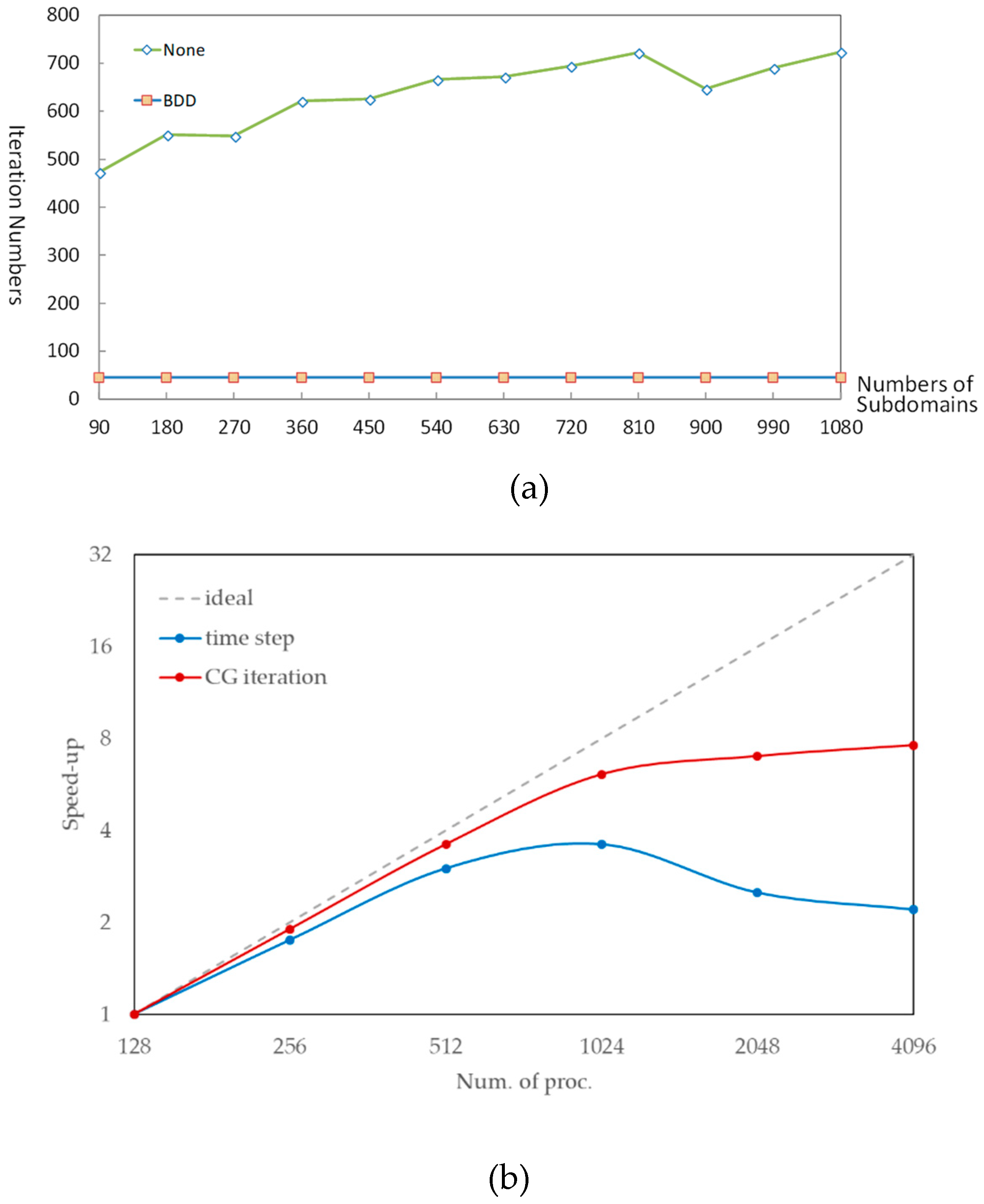
In order to evaluate the parallel scalability of the BDD preconditioners, a thermal-driven cavity problem is selected as the typical example to test the algorithm on the Tianhe-II supercomputer. Figure 1 presents the result of the numerical test, where “None” denotes the case without any preconditioner employed, and “BDD” denotes the case employing the BDD preconditioner introduced by Equation (17).
In the testing case, the model is divided into 80 parts (processor elements) in total, and the results are obtained from the tests with different numbers of subdomains in each part and 50,000 non-steady steps (the time step s).
The rapid growth of the condition number comes with the increasing of the amount of the subdomains is another reason to utilize BDD as a preconditioner of the problem. To assess the progress made by the BDD preconditioner, Figure 1a shows the result of a numerical scalability test. As the curve shows, the number of the BDD iterations remains at a low level, whereas the non-BDD iterations keep increasing as the number of the subdomains increases. Accordingly, the BDD preconditioner is proven to be more appropriate for large-scale computation for its excellent convergence. Nevertheless, a “trade-off” strategy is still necessary for parameterization. Figure 1b demonstrate the “strong scalability” test, including the speed-up of the CG iterations (denoted by “CG iteration”) and the non-stationary time step (denoted by “time step”) with a different number of processes. Excessive decomposition of the computation model would bring enormous memory consumption, which would restrict the growth of the parallel efficiency shown in Figure 1b.
3.2. An Indoor Ventilation Model
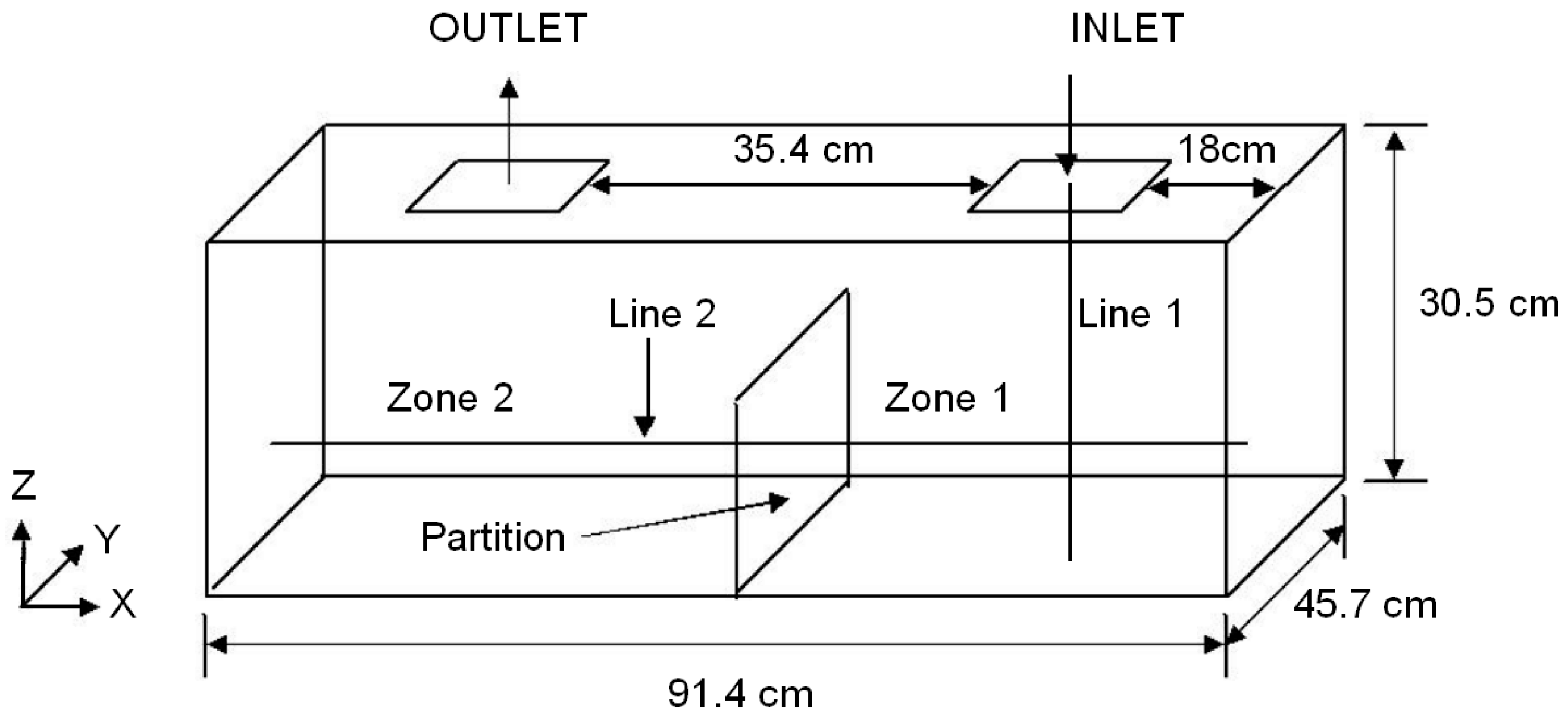
The experimental model is shown in Figure 2. The entire Zone is divided by a partition, and the right side is named as Zone 1 while the left side is named as Zone 2. There is a ventilation outlet in Zone 2 and a ventilation inlet in Zone 1. Both the inlet and outlet are ventilation ducts. A partition is located in the lower space of the middle of the room model, which is shown in Figure 2.
The reconstructed room model comes from the study of J. D. Posner, C. R. Buchanan, D. Dunn-Rankin* [3], the model has a floor area of 91.4 cm 45.7 cm with a height of 30.5 cm and a 15.25 cm high partition is built in the middle of the room to separate the two Zones. The horizontal cross-section area of ventilation inlet and ventilation outlet are both 10 cm 10 cm, and the height of both inlet and outlet ventilation ducts are 0.020m. Air enters the room from the inlet vent, flows through Zone 1 and Zone 2, eventually exits through the outlet vent.
3.3. Parameters and Conditions
The characteristic length of the inlet vent is0.1 m with the vertical inlet speed of . The relative pressure employed in the whole outlet vent and at a point on the inlet vent is set to zero. During the process of simulation, fluid temperature is held constant at 23 °C, which is the same as the temperature in the Lab when proceeding the measurement. Therefore, the coefficients in the equations can be considered as constants: the air density is , the concentration expansion coefficient is the kinematic viscosity is and the reference mass concentration is Based on Equation.
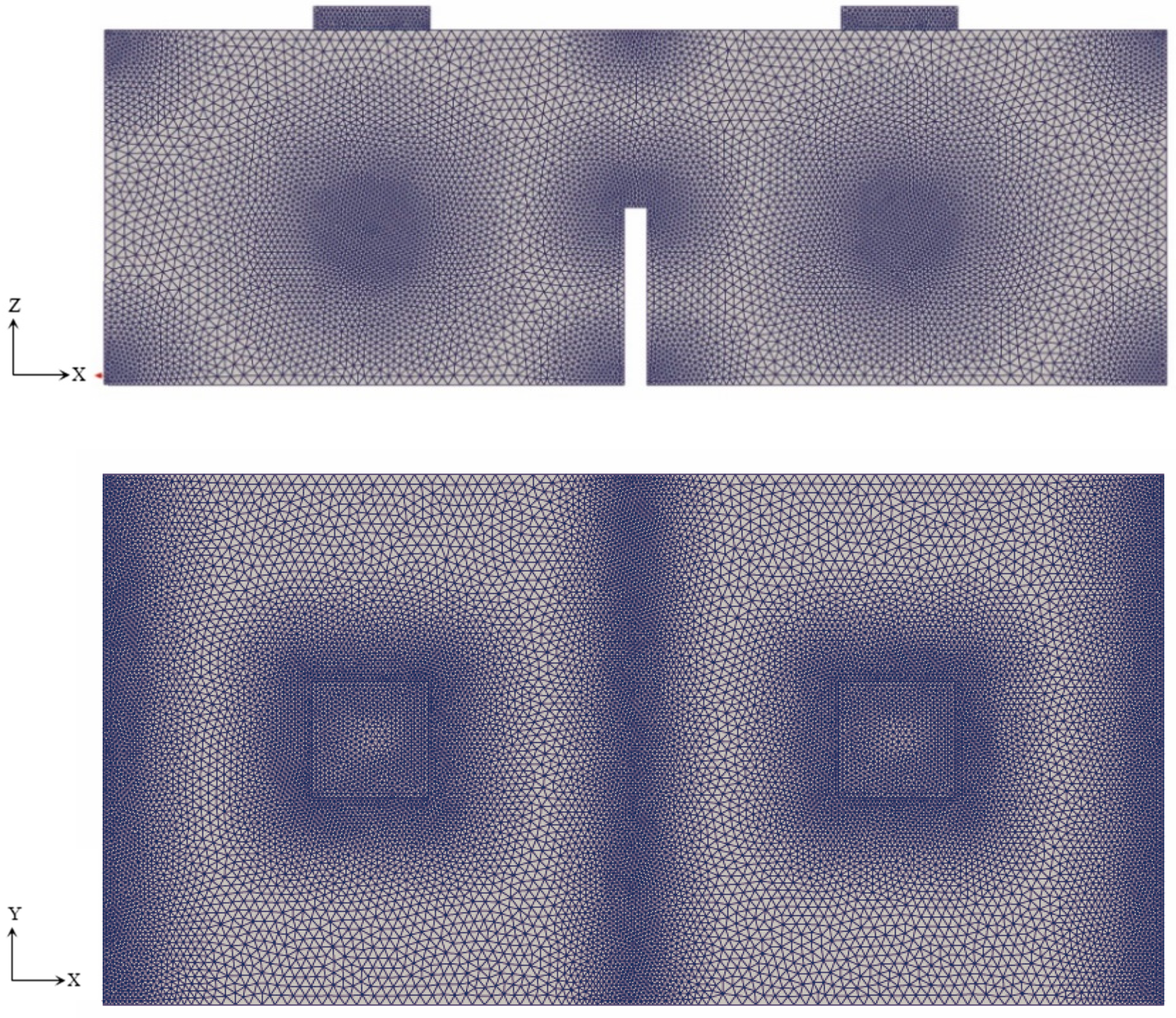
the Reynolds number of the inlet flow of this model is calculated to be . For a better setting of the Dirichlet boundary conditions, which can be applied on faces, edges or points, walls with thickness of 2 cm is constructed in the simulation, see the partition wall and the inlet and outlet vent in Figure 3. There are 20 faces in the model, and the velocity of air each face needs to be defined. Thus, the boundary condition at the ventilation outlet is set as the free boundary, and the velocity on the walls are defined as .
This study simulates the real condition of flow, and the velocity equals to 0 throughout the entire flow field as the initial condition. A grid convergence study of the DNS has been conducted. Time step size is set at , grid size equals to , and approximately 4170000 nodes are generated. The nodes number in the area of the inlet, outlet, corners of walls and corners of partition are tripled for the accuracy of the small vortex and the prevention of computation failure. The grid number and step size are the results of careful consideration of computational efficiency and accuracy. The mesh of the room model is shown in Figure 3.
According to the efficiency study in the above subsection, the model is set to be divided into 80 parts for optimal parallel efficiency on the computation platform.
4. Results and Analysis
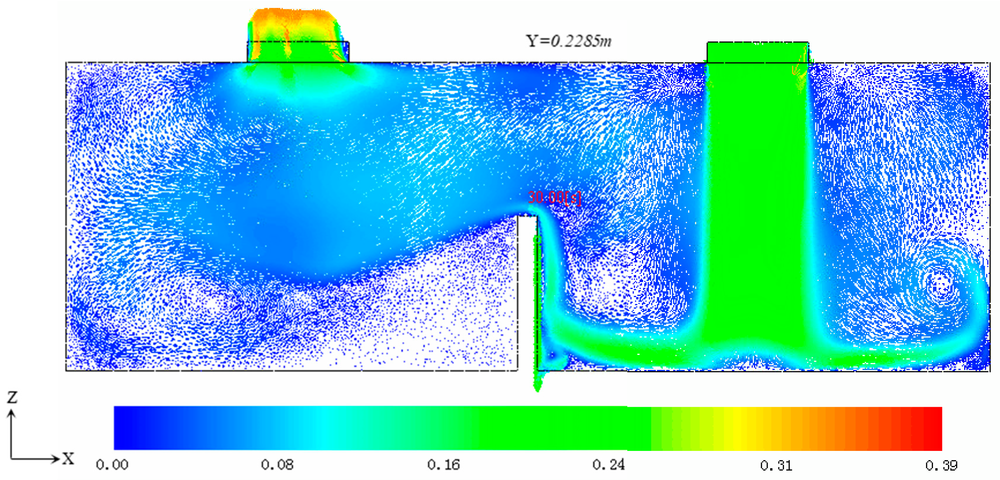
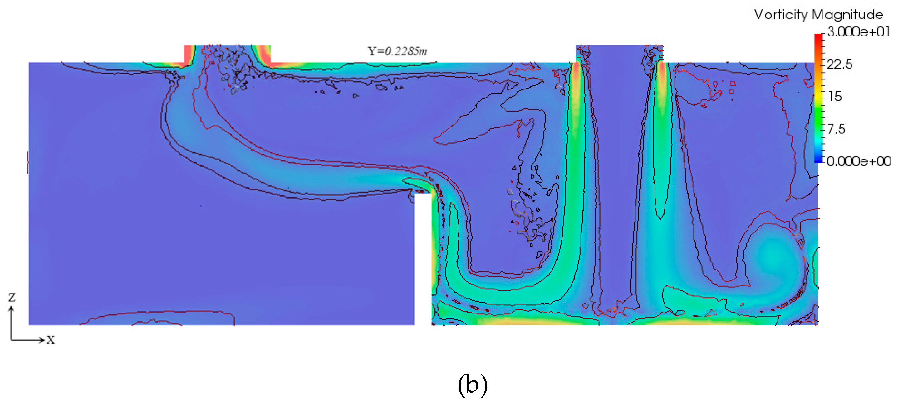
The stationary velocity field (at 30 s) on the vertical plane in the middle of the model room (the plane in Y = 0.2285 m) is shown in Figure 4. According to the result of the simulation, several features of flow are observed. The velocity of the jet stream from the inlet duct gradually decreases during the process of downward moving. Before touching the ground, the stream disperses into the direction away from Line 1 in space. It may be the reflect velocity of flow at the bottom that leads to the low-velocity area right under the jet stream, the velocity on Line 1 decreases from the inlet to the ground in the magnitude of approximately 100%. There are several local mini relatively high-velocity areas attached to the Zone 1 side of the partition. The airstream ascends on the partition and gradually disperses into Zone 2 with velocity decline. The velocity magnitude of air stream rapidly increases when approaching the outlet vent and the maximum magnitude of velocity reaches 0.39 m/s.
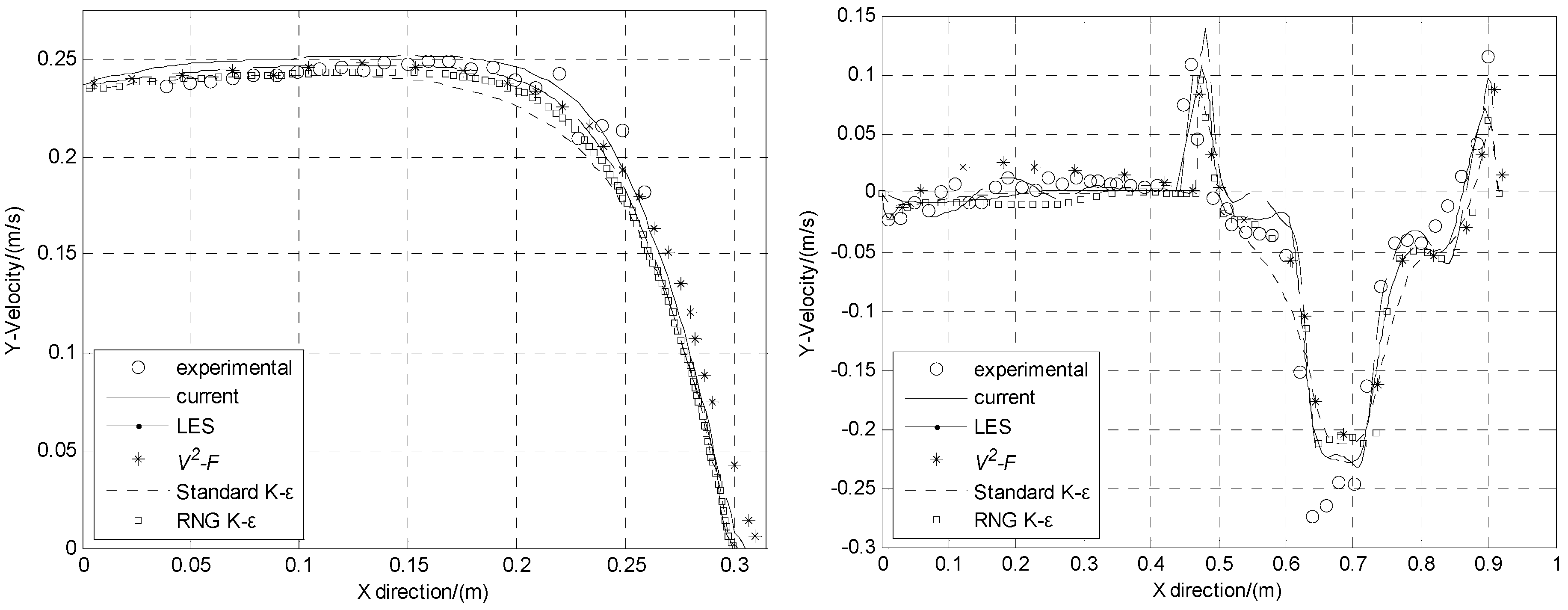
The comparison between air velocity in the vertical direction along Line 1 (the vertical inlet jet axis) and experimental data are presented in Figure 5. This figure shows that the data from DNS based on DDM (‘current’ in Figure 5) agree with the experiment data [6] and relatively more accurate in reflecting the velocity vary tendency, which means the current simulation result accurately represents the real velocity behavior of the flow.
The right part of Figure 5 shows the comparison between simulated and measured vertical velocity components along the horizontal Line 2 at mid-partition. According to the tendency of curves and points, the curve of the current result is better to approximate than other data sequences to the experimental result. Therefore, the reliability and efficiency of DNS based on DDM overweight it of model and other turbulence models.
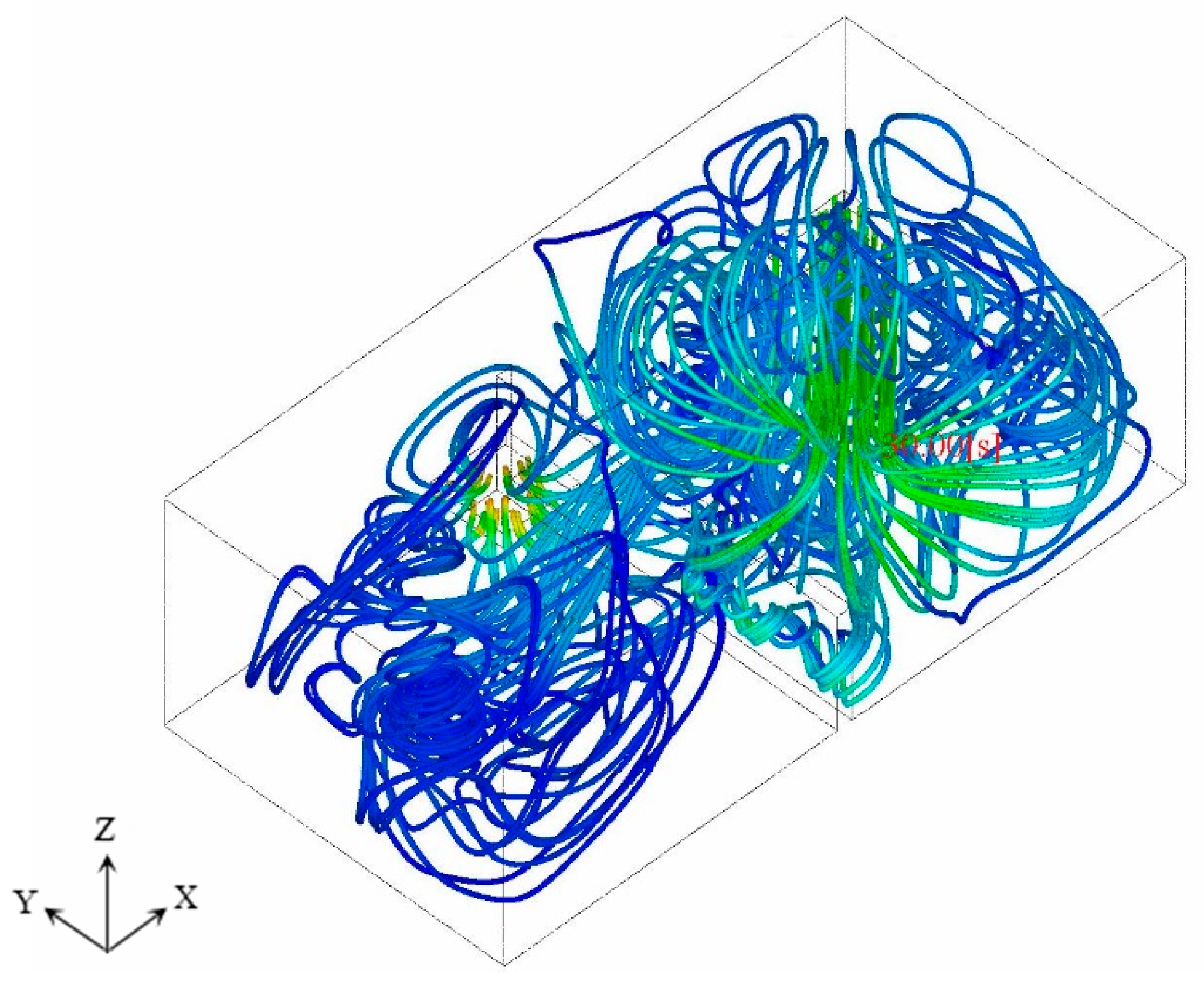
Figure 6 presents the streamline distribution in the steady phase in perceptive. The right rear of the model is Zone 1, and the left front of the model is Zone 2. The color system from warm to cool represents the absolute velocity from high to low. The following features can be observed: in Zone 1, the velocity magnitude of flow decreases with increasing distance from the inlet vent. Zone 1 is mainly controlled by higher-velocity flow, while Zone 2 is mostly occupied by lower velocity flow. Two large curvature of streamline with the lowest velocity exist near the end of Zone 2. Due to the symmetric model, the distribution of air streamlines in the whole room model is mainly symmetric.
These observations are reasonable: Firstly, the viscosity hinders the airflow from the inlet vent and decreases the speed of airflow. Moreover, the internal friction generated from the velocity gradient would also cause the shearing force and turbulence. Near the no-slip boundary in Zone 1, there exist long-term and almost symmetric eddies driven by the inlet flow. For Zone 2, the mechanical energy of airflow coming from Zone 1 has been dissipated, and the incoming airflow is at relatively low speed. The meddle-scale eddies generate near the partition and walls, which could raise the dust from Zone 1 into Zone 2 with pollutant and consequently assist the indoor ventilation. However, the low-velocity flow in Zone 2 cannot deliver the dust due to gravity. Furthermore, the small-scale eddies in Zone 2 generate the dust in a particular direction along the ground. It is what causes the dust and pollutant accumulation in a room.
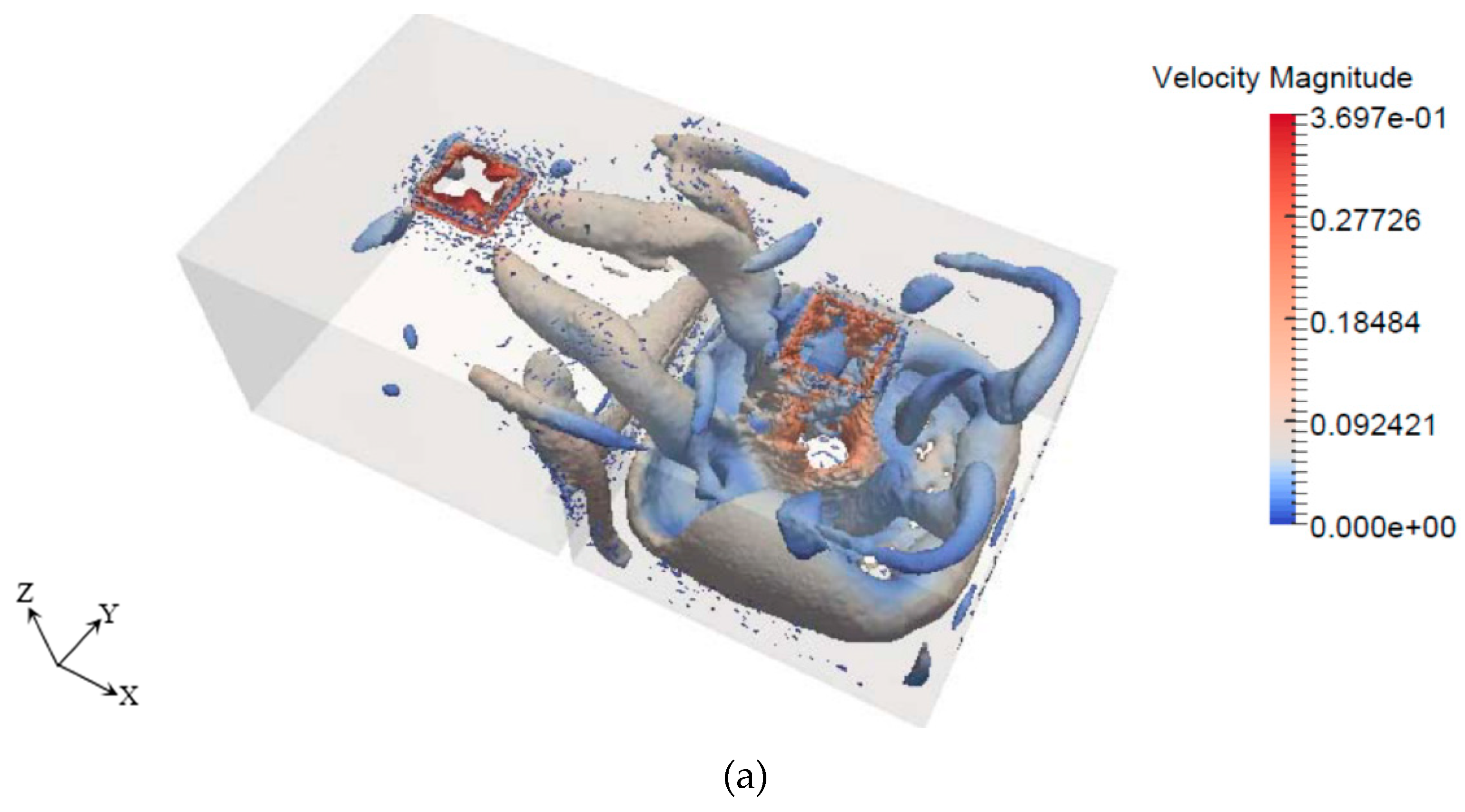
The vortex of the whole field is one of the essential factors to evaluate the ventilation rate of eddies because the vortex reflects the turbulent kinetic energy, which means the driven power of an eddy. According to the vortex field distribution shown in Figure 7, the highest value of vortex distributes around the main flow of the jet stream near the inlet duct, and more significantly, there are several obvious local mini strong-vortex areas over the bottom area of Zone 1. Figure 4 shows a tendency that the mainstream of airflow is forced to move along the surface of the wall in Zone 1 without touching it because the no-slip boundary setting at the wall prevents further approaches by the flow. Most space of Zone 2 has low vortex value except the area near the outlet vent. The triangle area distributed on the Zone 2 side of the partition is noticeable, and the high possibility of contaminant accumulation in this area is predictable. The vorticity is significantly smaller in the Zone 2, except for a noticeably large number of vortexes in the triangular area near the vent. Therefore, the high possibility of pollutant accumulation in the triangular area is predictable.
Overall, the DNS based on DDM proposed in this paper provides a new method to numerical simulate the airflows in a ventilated room since the results shown above have proved that this simulation is consistent with the experimental measurement. However, the discrepancy between the current simulation result and the experimental data in Figure 5 (left) shows that there is an inaccuracy of initial condition (distance less than 0.1 m) at the inlet vent. The cause of the inaccuracy is the thickness of the inlet (see details between Figure 2: An indoor ventilation model and Figure 3). At the beginning phase of the simulation, the initial value of relative pressure is set to be zero at a point on the inlet vent, which is 2 cm higher than the ceiling due to the thickness. The spatial difference of the model may cause the error in the numerical simulation. Fortunately, the influence of this factor can be approximately neglected, and the velocity magnitudes match the experimental data better than others simulation results when the airflow away from the inlet vent in Line 1 (distance greater than 0.1 m in the left part of Figure 5).
According to the comparison between current simulation and the simulation results conducted by other papers, the current simulation demonstrates higher accuracy and representative details of airflow behavior and vortex, which is of great importance in the improvement of indoor ventilation management.
5. Conclusions
A new method of DNS (Direct Numerical Simulation) based on DDM (Domain Decomposition Method) from our current algorithm is introduced in this paper for simulating the airflow patterns through modern building rooms. The flow of air in the ventilated room is simulated using a pressure stabilized scheme in a balancing domain decomposition (BDD) system. The proposed simulation model results are in close agreement with previously reported simulation data, and since the proposed simulation model shows more essential details than other models, such as the detailed information of velocity and vortex near the walls, the DNS based on DDM method is more accurate and reliable than model, large eddy simulation and methods.
The distribution of the vortex field shows that the distribution of air streamlines in the Zone 1 is different from Zone 2, and a relative vortex-free area exists on the Zone 2 side of the partition (Figure 2 shows how to partition the model and the definition of the Zones and Lines). The partition plays an essential role in changing the airflow behavior and its distribution. Based on the simulation results, four main phenomena are indicated: First of all, the inlet stream disperses into the direction away from Line 1 in space. The flow then ascends on the partition and gradually spreads into Zone 2 with velocity decline. Additionally, two large curvature of streamlines with the lowest velocity exist near the end of Zone 2. Moreover, the highest value of vortex distributes around the main flow of the jet stream locates at the bottom of Zone 1. Last but not least, the triangle area distributed on the Zone 2 side of the partition is noticeable, and the high possibility of dust accumulation in this area is predictable.
In this case, although only single-phase fluid is simulated, particles can be added into the simulation by applying a two-phase model. The distribution of particles affects the behavior of flow, and it also has a significant influence on the health of people in the room. The results of this paper lay a solid foundation for further study on the indoor airflow of a ventilated room. Further research is required to find out more elements that are essential to the relationship between a healthy indoor environment and the room structure.
Author Contributions
All authors contributed equally in the preparation of the present work.
Funding
This research was funded by the national key R&D program for international collaboration, grant number 2018YFE9103900 and for HPC, grant number 2016YFB0200603. Z. Jiang and J. Jiang were funded by the Natural Science Foundation of China (NSFC), grant number 11972384 and Guangdong MEPP Fund, grant number GDOE[2019] A01. A grant from Guangzhou Science and Technology program, grant number 201704030089, also supported this work.
Conflicts of Interest
The authors declare no conflict of interest.
References
- Asikainen, A.; Carrer, P.; Kephalopoulos, S.; Fernandes, E.D.; Wargocki, P.; Hänninen, O. Reducing burden of disease from residential indoor air exposures in Europe (HEALTHVENT project). Environ. Health A Glob. Access Sci. Source 2016, 15, 61–72. [Google Scholar] [CrossRef]
- Kim, E.H.; Kim, S.; Lee, J.H.; Kim, J.; Han, Y.; Kim, Y.M.; Ahn, K. Indoor Air Pollution Aggravates Symptoms of Atopic Dermatitis in Children. PLoS ONE 2015, 10, e0119501. [Google Scholar] [CrossRef] [PubMed]
- Meng, F.; Wu, H. Indoor Air Pollution by Methylsiloxane in Household and Automobile Settings. PLoS ONE 2015, 10, e0135509. [Google Scholar] [CrossRef] [PubMed]
- Ye, X.; Peng, L.; Kan, H.; Wang, W.; Geng, F.; Mu, Z.; Yang, D. Acute Effects of Particulate Air Pollution on the Incidence of Coronary Heart Disease in Shanghai, China. PLoS ONE 2016, 11, e0151119. [Google Scholar] [CrossRef] [PubMed]
- Xu, Q.; Li, X.; Wang, S.; Wang, C.; Huang, F.; Gao, Q.; Guo, X. Fine Particulate Air Pollution and Hospital Emergency Room Visits for Respiratory Disease in Urban Areas in Beijing, China, in 2013. PLoS ONE 2016, 11, e0153099. [Google Scholar] [CrossRef] [PubMed]
- Posner, J.D.; Buchanan, C.R.; Dunn-Rankin, D. Measurement and prediction of indoor air flow in a model room. Energy Build. 2003, 35, 515–526. [Google Scholar] [CrossRef]
- Friedlander, S.K.; Marlow, W.H. Smoke, Dust and Haze: Fundamentals of Aerosol Behavior. Phys. Today 2000, 30, 58–59. [Google Scholar] [CrossRef]
- Tong, Z.; Chen, Y.; Malkawi, A.; Adamkiewicz, G.; Spengler, J.D. Quantifying the impact of traffic-related air pollution on the indoor air quality of a naturally ventilated building. Environ. Int. 2016, 89–90, 138–146. [Google Scholar] [CrossRef]
- Cheong, K.W.D.; Djunaedy, E.; Poh, T.K.; Tham, K.W.; Sekhar, S.C.; Wong, N.H.; Ullah, M.B. Measurements and computations of contaminant’s distribution in an office environment. Build. Environ. 2003, 38, 135–145. [Google Scholar] [CrossRef]
- Chung, K.C. Three-dimensional analysis of airflow and contaminant particle transport in a partitioned enclosure. Build. Environ. 1998, 34, 7–17. [Google Scholar] [CrossRef]
- Lu, W.; Howarth, A.T. Numerical analysis of indoor aerosol particle deposition and distribution in two-zone ventilation system. Build. Environ. 1996, 31, 41–50. [Google Scholar] [CrossRef]
- Cehlin, M.; Karimipanah, T.; Larsson, U. "Unsteady CFD simulations for prediction of airflow close to a supply device for displacement ventilation. In Proceedings of the 13th International Conference on Indoor Air Quality and Climate, Indoor Air 2014, Hong Kong, China, 7–12 July 2014; p. 47. [Google Scholar]
- Chen, Q. Using computational tools to factor wind into architectural environment design. Energy Build. 2004, 36, 1197–1209. [Google Scholar] [CrossRef]
- Bogodage, S.G.; Leung, A.Y.T. CFD simulation of cyclone separators to reduce air pollution. Powder Technol. 2015, 286, 488–506. [Google Scholar] [CrossRef]
- Ioannis, K.P.; Athanasios, N.K.; Pavlos, K.; Kostantinos, A. A CFD Simulation Study of VOC and Formaldehyde Indoor Air Pollution Dispersion in an Apartment as Part of an Indoor Pollution Management Plan. Aerosol Air Qual. Res. 2011, 11, 758. [Google Scholar]
- Jiang, Y.; Alexander, D.; Jenkins, H.; Arthur, R.; Chen, Q. Natural ventilation in buildings: Measurement in a wind tunnel and numerical simulation with large-eddy simulation. J. Wind Eng. Ind. Aerodyn. 2003, 91, 331–353. [Google Scholar] [CrossRef]
- Kobayashi, T.; Sugita, K.; Umemiya, N.; Kishimoto, T.; Sandberg, M. Numerical investigation and accuracy verification of indoor environment for an impinging jet ventilated room using computational fluid dynamics. Build. Environ. 2017, 115, 251–268. [Google Scholar] [CrossRef]
- Pulat, E.; Ersan, H.A. Numerical simulation of turbulent airflow in a ventilated room: Inlet turbulence parameters and solution multiplicity. Energy Build. 2015, 93, 227–235. [Google Scholar] [CrossRef]
- Pavarino, L.; Widlund, O. Balancing Neumann-Neumann Methods for Incompressible Stokes Equations. Commun. Pure Appl. Math. 2002, 55, 302–335. [Google Scholar] [CrossRef]
- Yudison, A.P.; Driejana, R. Development of Indoor Air Pollution Concentration Prediction by Geospatial Analysis. J. Eng. Technol. Sci. 2015, 47, 306–319. [Google Scholar]
- Kao, H.-M.; Chang, T.-J.; Hsieh, Y.-F.; Wang, C.-H.; Hsieh, C.-I. Comparison of airflow and particulate matter transport in multi-room buildings for different natural ventilation patterns. Energy Build. 2009, 41, 966–974. [Google Scholar] [CrossRef]
- Guerra, D.R.S.; Su, J.; Freire, A.P.S. The near wall behavior of an impinging jet. Int. J. Heat Mass Transf. 2005, 48, 2829–2840. [Google Scholar] [CrossRef]
- Piomelli, U. Large-eddy simulation: Achievements and challenges. Prog. Aerosp. Sci. 1999, 35, 335–362. [Google Scholar] [CrossRef]
- Zhang, W.; Chen, Q. Large eddy simulation of indoor airflow with a filtered dynamic subgrid scale model. Int. J. Heat Mass Transf. 2000, 43, 3219–3231. [Google Scholar] [CrossRef]
- Tian, Z.F.; Tu, J.Y.; Yeoh, G.H.; Yuen, R.K.K. Numerical studies of indoor airflow and particle dispersion by large Eddy simulation. Build. Environ. 2007, 42, 3483–3492. [Google Scholar] [CrossRef]
- Lu, W.; Howarth, A.T.; Adam, N.; Riffat, S.B. Modelling and measurement of airflow and aerosol particle distribution in a ventilated two-zone chamber. Build. Environ. 1996, 31, 417–423. [Google Scholar] [CrossRef]
- Chang, T.-J.; Hsieh, Y.F.; Kao, H.M. Numerical investigation of airflow pattern and particulate matter transport in naturally ventilated multi-room buildings. Indoor Air 2006, 16, 136–152. [Google Scholar] [CrossRef]
- Durbin, P.A. Separated flow computations with the k-epsilon-v-squared model. AIAA J. 1995, 33, 659–664. [Google Scholar] [CrossRef]
- Li, K.; Gong, G. Numerical simulation of indoor suspension particles based on v2-f model. Appl. Math. Model. 2012, 36, 2510–2520. [Google Scholar] [CrossRef]
- Choi, J.; Hur, N.; Kang, S.; Lee, E.D.; Lee, K.-B. A CFD simulation of hydrogen dispersion for the hydrogen leakage from a fuel cell vehicle in an underground parking garage. Int. J. Hydrog. Energy 2013, 38, 8084–8091. [Google Scholar] [CrossRef]
- Yao, Q.; Zhu, Q. A Pressure-Stabilized Lagrange-Galerkin Method in a Parallel Domain Decomposition System. Abstr. Appl. Anal. 2013, 2013, 161873. [Google Scholar] [CrossRef]
- Brezzi, F.; Fortin, M. Mixed and Hybrid Finite Element Methods; Springer: New York, NY, USA, 1991; p. 350. [Google Scholar]
- Qinghe, Y.; Kanayama, H. A Coupling Analysis of Thermal Convection Problems Based on a Characteristic Curve Method. Theor. Appl. Mech. Jpn. 2011, 59, 257–264. [Google Scholar]
- Farhat, C.; Roux, F.X.; Mechanics, I.A.F.C.; Oden, J.T. Implicit Parallel Processing in Structural Mechanics; North-Holland: North Holland, Holland, 1994. [Google Scholar]
- Mandel, J. Balancing domain decomposition. Commun. Numer. Methods Eng. 1993, 9, 233–241. [Google Scholar] [CrossRef]
- Shioya, R.; Ogino, M.; Kanayama, H.; Tagami, D. Large scale finite element analysis with a Balancing Domain Decomposition method. In Progress in Experimental and Computational Mechanics in Engineering; Geni, M.K.M., Ed.; Key Engineering Materials; Trans Tech Publications: Zurich, Switzerland, 2003; Volume 243, pp. 21–26. [Google Scholar]
- Mukaddes, A.M.M.; Ogino, M.; Kanayama, H.; Shioya, R. A Scalable Balancing Domain Decomposition Based Preconditioner for Large Scale Heat Transfer Problems. JSME Int. J. Ser. BFluids Therm. Eng. 2006, 49, 533–540. [Google Scholar] [CrossRef]
- Yao, Q.; Kanayama, H.; Ognio, M.; Notsu, H. Incomplete Balancing Domain Decomposition for Large scale 3-D non-stationary incompressible flow problems. IOP Conf. Ser. Mater. Sci. Eng. 2010, 10, 012029. [Google Scholar] [CrossRef]
- Yao, Q.; Zhu, Q. Investigation of the Contamination Control in a Cleaning Room with a Moving AGV by 3D Large-Scale Simulation. J. Appl. Math. 2013, 2013, 570237. [Google Scholar] [CrossRef] [Green Version]
Figure 1.
Parallel efficiency (a) and speed up (b) of the current algorithm.

Figure 2.
An indoor ventilation model.

Figure 3.
details of meshing: front view (upper) and top view (lower).

Figure 4.
Vectors of flow velocity, the color bar number represents the velocity magnitude (m/s).

Figure 5.
Comparison of velocity along Line 1 (left) and Line 2 (right).

Figure 6.
Streamline at 30 s.

Figure 7.
Isosurface of vortex field at 30 s (a) vortex contour in the plane Y = 0.2285 m (b).


© 2019 by the authors. Licensee MDPI, Basel, Switzerland. This article is an open access article distributed under the terms and conditions of the Creative Commons Attribution (CC BY) license (http://creativecommons.org/licenses/by/4.0/).
Share and Cite
MDPI and ACS Style
Jiang, J.; Jiang, Z.; Kwan, T.H.; Liu, C.-H.; Yao, Q. Study of Indoor Ventilation Based on Large-Scale DNS by a Domain Decomposition Method. Symmetry 2019, 11, 1416. https://0-doi-org.brum.beds.ac.uk/10.3390/sym11111416
AMA Style
Jiang J, Jiang Z, Kwan TH, Liu C-H, Yao Q. Study of Indoor Ventilation Based on Large-Scale DNS by a Domain Decomposition Method. Symmetry. 2019; 11(11):1416. https://0-doi-org.brum.beds.ac.uk/10.3390/sym11111416
Chicago/Turabian StyleJiang, Junyang, Zichao Jiang, Trevor Hocksun Kwan, Chun-Ho Liu, and Qinghe Yao. 2019. "Study of Indoor Ventilation Based on Large-Scale DNS by a Domain Decomposition Method" Symmetry 11, no. 11: 1416. https://0-doi-org.brum.beds.ac.uk/10.3390/sym11111416
Note that from the first issue of 2016, this journal uses article numbers instead of page numbers. See further details here.