Material Symmetries in Homogenized Hexagonal-Shaped Composites as Cosserat Continua


1
DICAM Department, University of Bologna, 40136 Bologna, Italy
2
DISG Department, Sapienza University of Rome, 00185 Rome, Italy
3
Engineering Department, Parthenope University of Naples, 80133 Naples, Italy
*
Author to whom correspondence should be addressed.
Symmetry 2020, 12(3), 441; https://0-doi-org.brum.beds.ac.uk/10.3390/sym12030441
Submission received: 4 February 2020
/
Revised: 4 March 2020
/
Accepted: 7 March 2020
/
Published: 10 March 2020
(This article belongs to the Special Issue Time and Space Nonlocal Operators in Structural Mechanics)
Abstract
:In this work, material symmetries in homogenized composites are analyzed. Composite materials are described as materials made of rigid particles and elastic interfaces. Rigid particles of arbitrary hexagonal shape are considered and their geometry described by a limited set of parameters. The purpose of this study is to analyze different geometrical configurations of the assemblies corresponding to various material symmetries such as orthotetragonal, auxetic and chiral. The problem is investigated through a homogenization technique which is able to carry out constitutive parameters using a principle of energetic equivalence. The constitutive law of the homogenized continuum has been derived within the framework of Cosserat elasticity, wherein the continuum has additional degrees of freedom with respect to classical elasticity. A panel composed of material with various symmetries, corresponding to some particular hexagonal geometries defined, is analyzed under the effect of localized loads. The results obtained show the difference of the micropolar response for the considered material symmetries, which depends on the non-symmetries of the strain and stress tensor as well as on the additional kinematical and work-conjugated statical descriptors. This work underlines the importance of resorting to the Cosserat theory when analyzing anisotropic materials.
1. Introduction
In the study of composite materials, symmetries play a very important role in identify symmetry planes and peculiar material behaviors. It is well-known that composite materials can be investigated by directly analyzing their constituents in a micromechanical model or by homogenizing them as an equivalent continuum. For composites made of particles and matrix, for instance, the analysis of the single constituents might require high computational cost [1,2]. On the contrary, homogenization is faster and more efficient, but the effectiveness of such a way has to be validated and modeled using proper continuum theories [3,4,5,6]. In particular, the homogenization of complex interaction effects in composite materials needs internal scale parameters which are not negligible compared to the structural length scale.
The paper [7] describes a historical overview of different homogenization techniques which have been extended to non-classical continua. As it is well known in the literature, the classical continuum, by lacking in internal lengths, leads to ill-posed problems. This calls for the need of non-local descriptions which include internal length parameters in different ways; or by adding extra degrees of freedom, thus obtaining the so-called implicit/weak non-local descriptions, or by adding extra parameter as internal variables, obtaining the so-called explicit/strong non-local descriptions [8,9]. The latter aim to account for material nonlocality without modifying classical kinematics [10,11,12,13].
Multiscale computational homogenization proposed in [14,15,16,17,18,19,20,21] used non-local or higher order deformation gradient theories in composite materials. In addition, non-local explicit modeling in elastic composites were presented in [22,23,24,25]. Non-local models with gradient elasticity can be used to study one-dimensional structures such as beams [26,27,28] and rods [29,30].
On the other hand, within the framework of implicit non-local theories concerning models with additional degrees of freedom [7,8,9], micromorphic continua, in particular continua with rigid local structures (micropolar), have been satisfactorily applied to various composites [31,32,33,34,35,36,37,38,39,40,41].
All the aforementioned non-local models are then defined as non-local because the governing equations contain one or more parameters that inherit a micro-structural character which affects the macroscopic behavior and because of dispersion properties in wave propagation [42,43,44,45,46]. Numerical simulations can be performed by fitting numerical experiments which have a physical evidence of the presence of such non-locality.
When classical kinematics are enriched with extra degrees of freedom, in many cases, homogenization procedures have been shown to provide more reliable models than in the case of classical local continua [43,47]. In the present work, micropolar theory is considered which introduces the rotation of the material point, termed microrotation, to be distinguished with the macrorotation of the body (local rigid rotation). The effects of this local rotation have been widely investigated in [38,39,48,49,50] for masonry-like materials.
In the recent literature, the couple-stress theory has been widely used for several applications [35,51,52], however, in this theory, micro and macro rotation coincide and when couple stresses are negligible, classical elasticity theory is derived (see appendix in [31]). As it has been also recently analyzed by [53], micro-polar effects become prominent when geometrical or load singularities are present in the reference problem, such as concentrated loads, voids or material inclusions. These effects have been also compared to those of of explicit non-local continuum descriptions [8,9].
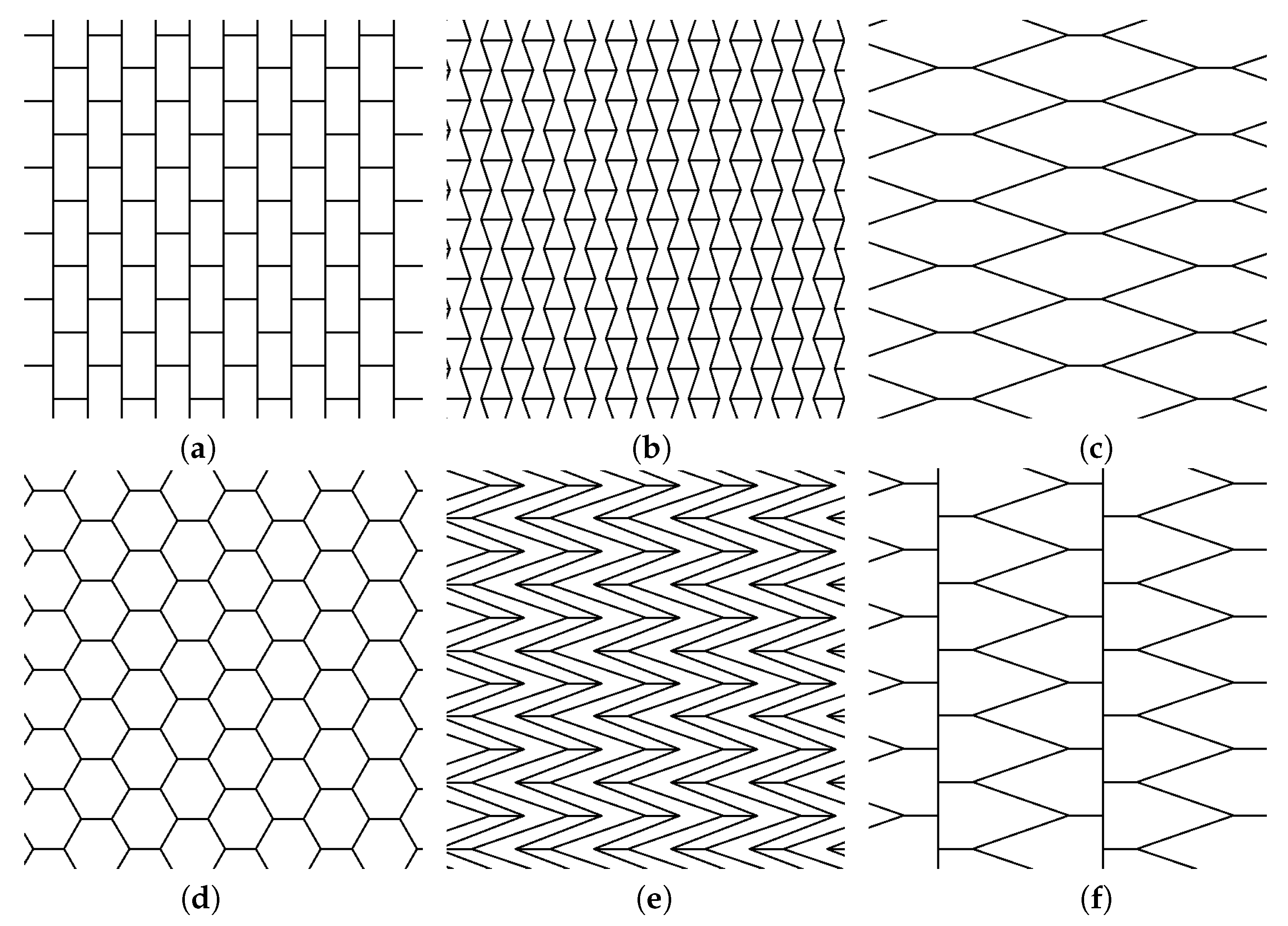
The present work investigates the behavior of hexagonal lattices with elastic interfaces homogenized as equivalent Cosserat continua [54,55]. According to the hexagonal geometry selected for a generic tile (e.g., orientation of the interfaces and internal angles of the hexagonal geometry), distinct material symmetries can be derived [56,57]. With reference to the hexagonal parametrization available in [58], classes of hexagonal geometries are investigated. Among these, six geometries are analyzed; they all have different peculiarities such as those pertaining to orthotropic, orthotetragonal, auxetic and chiral aspects. These geometries are defined as rectangular, hourglass, diamond, regular (hexagonal), skew and tip. All these shapes derive from the regular hexagonal geometry with equal edges by changing two internal angles.
First, contour maps of the possible hexagonal configurations are displayed in order to globally analyze mechanical properties of the equivalent solids. Second, a solid wall made of six selected hexagonal tiles is analyzed under a concentrated load in order to achieve micropolar behavior of the wall as a function of the microstructure.
This paper is divided into the four sections described below. First, the Cosserat continuum model is briefly presented in order to introduce current quantities and symbols. Second, a parametric hexagonal geometry based on four parameters is presented and the investigated patterns are shown and defined. Third, an in-house finite element implementation is presented using linear finite elements with reduced integration. Finally, numerical applications are discussed by comparison among the six considered geometries and physical deduction from the contour plots are given. Paper conclusions and remarks are given in the conclusion section.
2. Framework of Cosserat Theory
In the present work, a two-dimensional framework is considered for simplicity. The Cosserat kinematics take into account an additional degree of freedom of particle rotation other than classical displacement components and .
The kinematic compatibility equations in matrix form are
where , and are the strain components: axial, angular and curvature ordered in the strain vector . Note that the angular strain components are not reciprocal, . In general in the micropolar model the microrotation, , is different from the local rigid rotation (macrorotation), , defined as the skew-symmetric part of the gradient of displacement, and the difference between the two rotations, , defines the strain measure of the relative rotation that corresponds to the skew-symmetric part of the strain. When the relative rotation equals zero, , , the micropolar continuum becomes a continuum with constrained rotations [31,59]. In the following, we focus on as a peculiar strain measure of the micropolarity of the model under study.
The work conjugate stress vector to is written in the form , where for represent the normal and shear stress components, and , the microcouples. The stress components are not reciprocal, , and the couple stress components, , , have to be introduced in order to satisfy the moment equilibrium of the micropolar body. The Principle of Virtual Works can be written as
where and are the vectors of body forces and boundary tractions, respectively. Balance equations and correspondent boundary conditions can be carried from Equation (2).
For the sake of conciseness, boundary terms are not reported. For further details and reading, strong form equations can be found in [50,60,61].
The micropolar constitutive equations take the compact form
and extended matrix form
Due to hyperelasticity, the constitutive matrix in Equation (5) is symmetrical. This matrix is obtained via an energetic homogenization technique presented in [47]. Such homogenization starts from the definition of a Representative Volume Element (RVE) in which orientation and location of elastic interfaces are defined according to a hexagonal geometry selected and described in Section 4. Further details on constitutive elastic terms are given in the following sections.
3. Finite Element Implementation
A standard finite element implementation is considered for the numerical solution of the present Cosserat problem. The numerical framework follows the previous contributions of the authors [50,60,61]. An in-house finite element MATLAB code has been developed as an extension of a classical two-dimensional elastic continuum as given in [62].
A linear finite element model is considered with quadrilateral (Q4) elements. Linear Lagrange interpolation functions are used; thus, the approximation takes the form , where is the vector of degrees of freedom of the model, is the matrix of shape functions (of size ) and the vector of nodal displacements.
By inserting the finite element approximation in the strain definitions (1) and in the variational form of the equilibrium (2) the stiffness matrix and load vectors can be derived as
where is the matrix which includes the derivatives of the shape functions. Note that selective Gauss integration is performed on the shear terms due to different differentiation orders among displacements and rotational approximation. In the present work, body forces are neglected and this is why they do not appear in the force vector definition above.
The present finite element approximation is based on displacements; therefore, derivative quantities are post-computed according to a Gauss–Legendre grid, and inter-element averaging is done in the nodes without any extra weight [60].
4. Numerical Applications
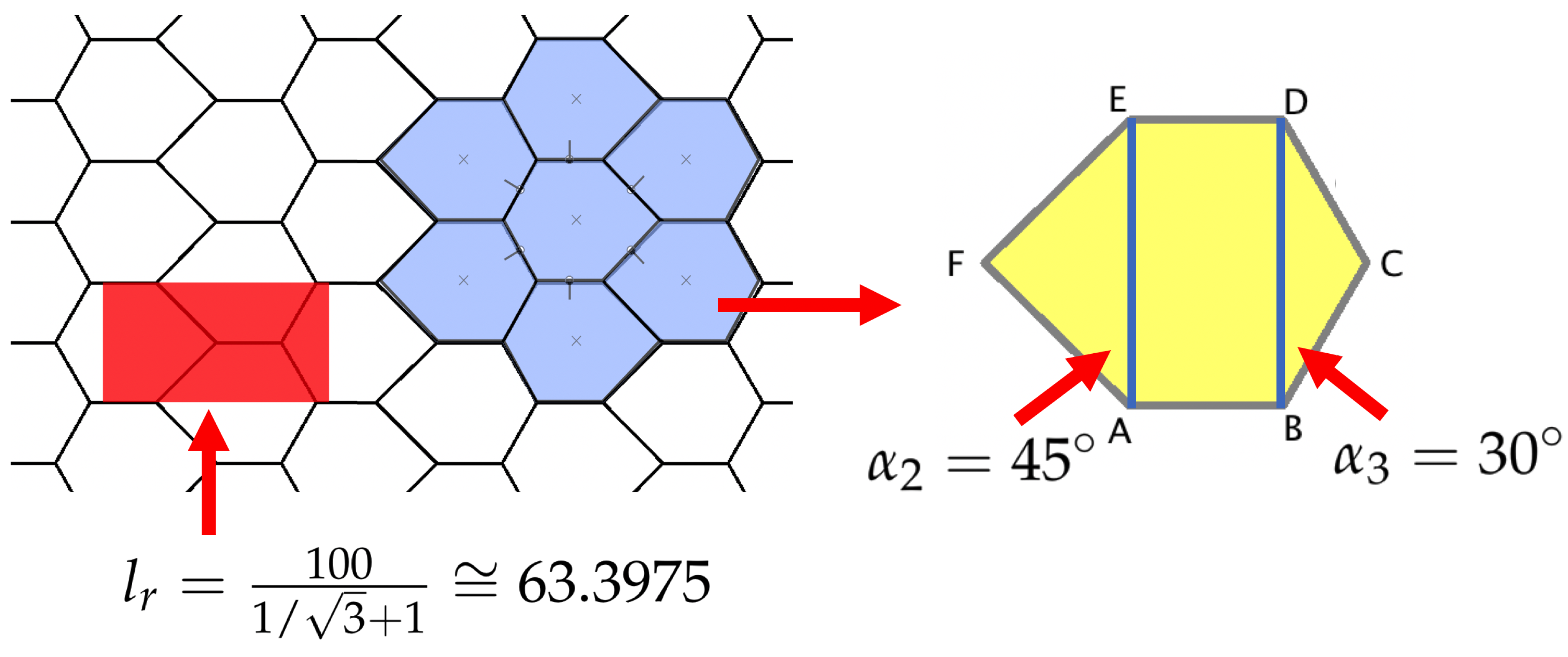
The hexagonal pattern of Figure 1 has been defined according to the parametrization [58]. The single tile is defined by the relative length which identifies the unit parallelogram. The selected RVE is highlighted within the centroids of the tiles and outward unit normal vectors at the block interfaces used for computing the constitutive matrix according to the procedure presented by [47].
In the following, relative length and the angles , are variable (Figure 1). The relative length defines the ratio between and . The single tile is defined by a rectangle and two isosceles triangles with the base attached to BD and AE edges of the rectangle. The nodal coordinates of the single tile are given by:
- ,
- ,
- ,
- ,
- ,
where , , , . Due to this definition, the geometric range of parameters and is [].
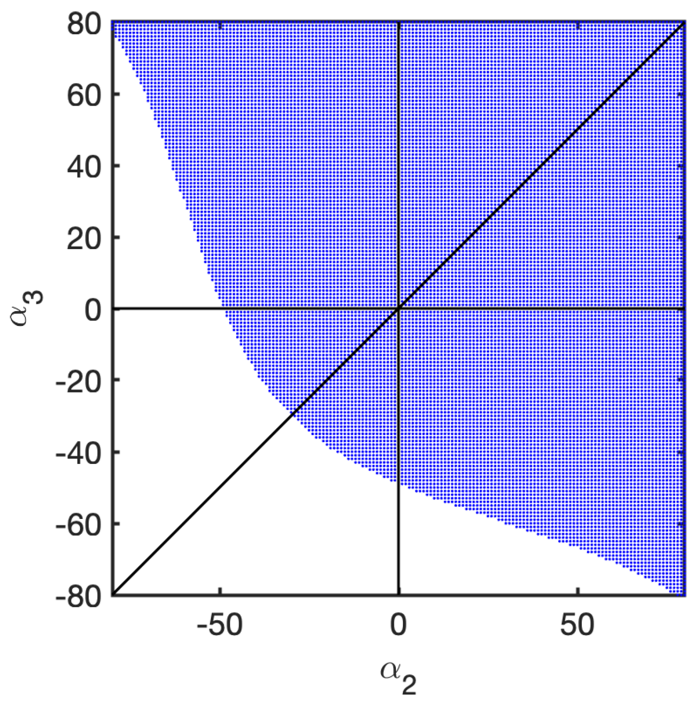
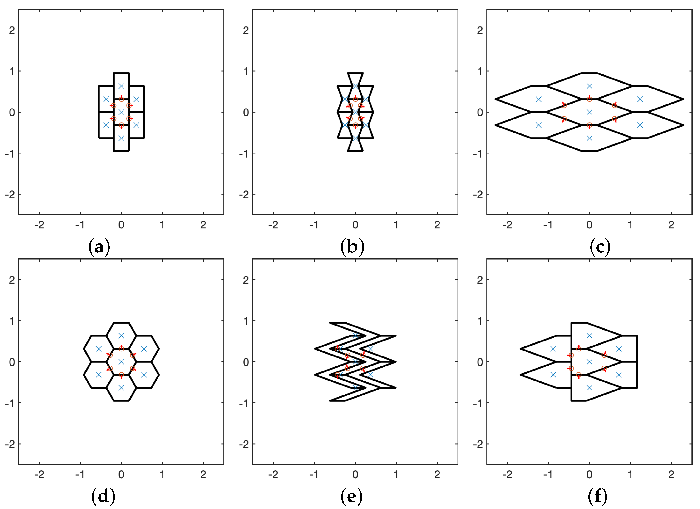
Thus, by keeping the relative length constant and varying and , all possible configurations (not self-intersecting hexagons) are depicted in Figure 2. Note that the main diagonal represents the case wherein and the horizontal and vertical lines represent and , respectively. The two orthogonal lines divide the space in four areas:
- The upper-right area has and where any combination is theoretically possible in the given domain range. In this area, regular hexagons are present as well as diamond shaped ones (according to Figure 3).
- The lower-left area has and where not all shapes are achievable due to some self-intersections of hexagons. In this area, hourglass shaped hexagons are present (symmetric and not-symmetric ones) according to Figure 3.
- The upper-left and lower-right areas have and and and , respectively. These shapes might be characterized by an asymmetric shape (according to Figure 3).
The constitutive matrices of several hexagonal configurations are considered in the following. The homogenization procedure follows the approach described by [47], where the adopted spring stiffness values at the elastic joint interfaces are . Energetic equivalence is used to carry out rotational stiffness as:
where d is the current interface length between two rigid particles in contact, for which the interactive stiffness is computed. Note that the definition of is a particular choice which depends on the Poisson coefficient of the heterogeneous medium.
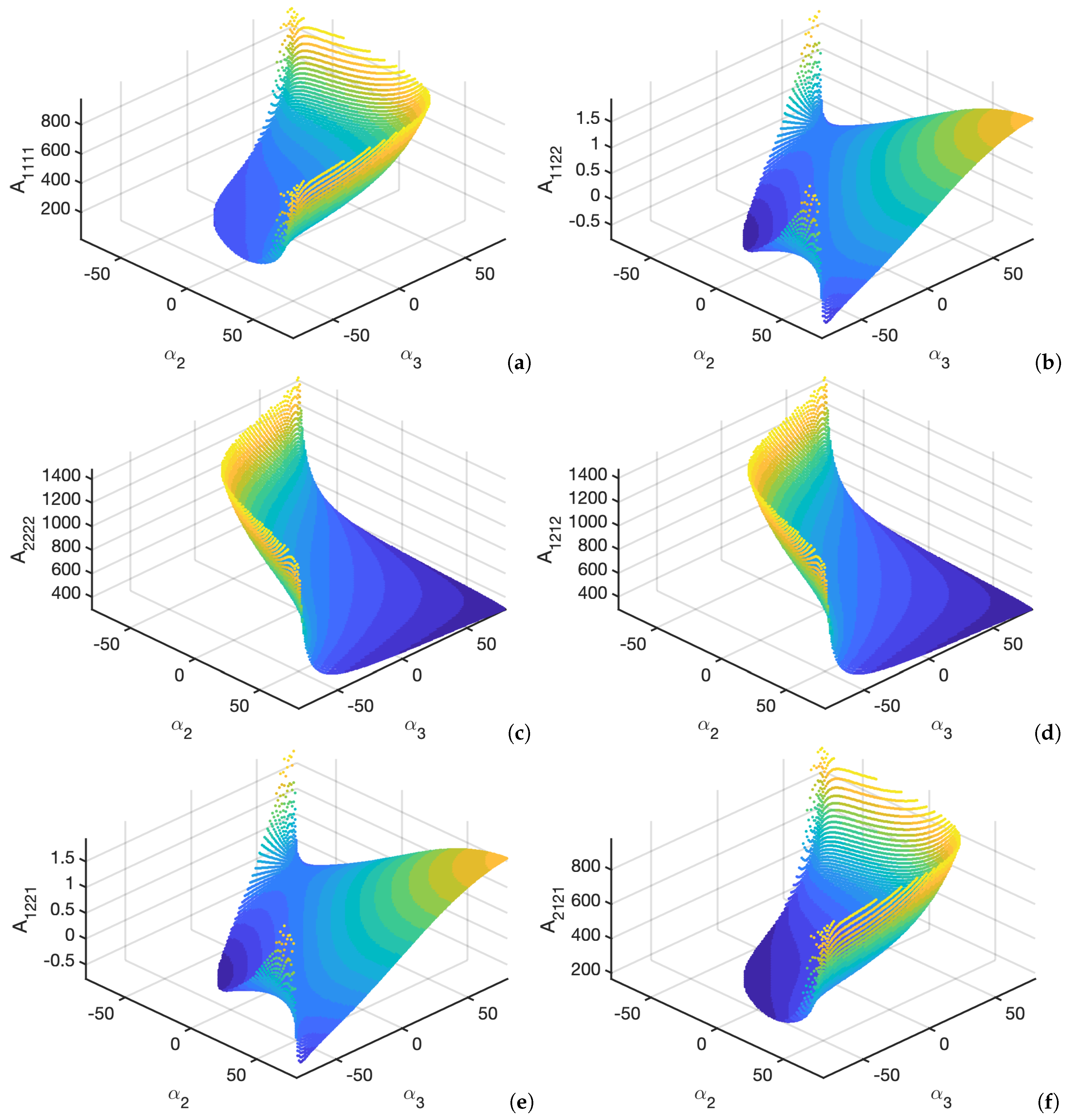
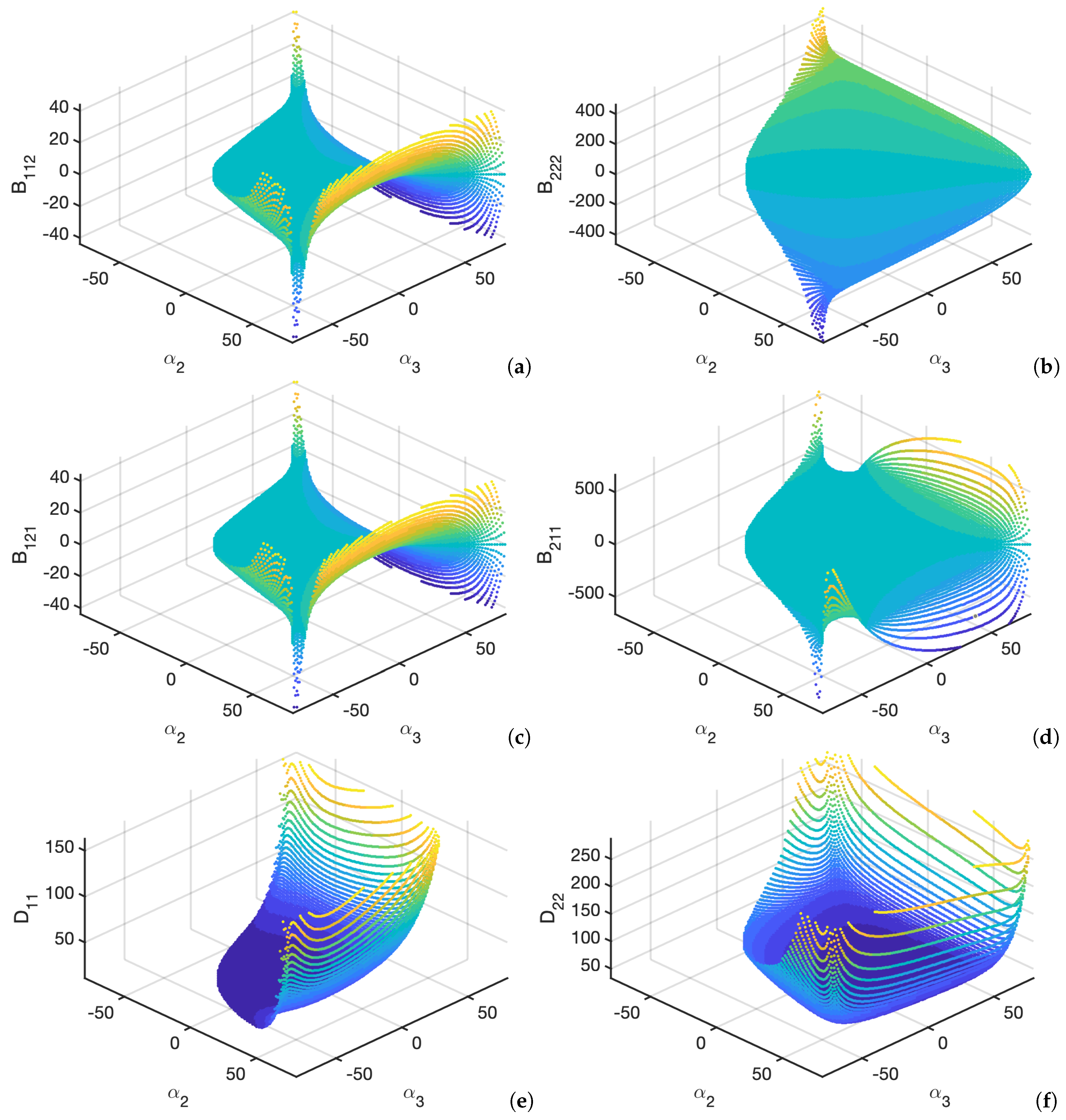
Considering all the possible geometric configurations illustrated in Figure 2 the equivalent mechanical properties of the equivalent micropolar material can be carried out according to the constitutive matrix (5) as in [50,61]. The nonzero components of the classical constitutive matrix are depicted in Figure 4. Please note that for all possible hexagonal combinations, . Similar trends are observed for and , as well as the couples and , finally for and as shown in Figure 4. Note that stiffnesses on the main diagonal are related (as well as off-diagonal terms which are related to Poisson effect and shear asymmetry). and increase as or increase on the contrary and have an opposite behavior (they increase when the two angles decrease). Off-diagonal terms and are positive when ; they have negative values otherwise. Positive or negative values are also observed when and vice versa. The latter occur for asymmetric configurations of the tiles according to the nomenclature introduced in [60].
Coupling between stresses/curvatures and microcouples/strains are observed when chiral material behavior is present. As presented in [60], chiral behavior occurs when asymmetric tiles are considered for . As a matter of fact, components are zero for as depicted in Figure 5a–d. Positive or negative values of are observed only if , larger for large values of angles, thus for high skewness of the tiles. Finally, in Figure 5e,f the micro-couple stiffness are shown which are high for large values of and , no matter their sign.
Thus the constitutive relations for the present case are always in the form
Given the aforementioned presentation of the constitutive configurations, the results for the following material configurations are shown:
- rectangular:
- hourglass:
- diamond:
- regular:
- skew:
- tip: ,
And their reference RVE is depicted in Figure 6. The constitutive matrices of the configurations selected and depicted in Figure 6 are listed below. For the rectangular configuration, it is
An orthotropic nature of the material is observed when rectangular tiles are considered [31,47] (Figure 6a).
The constitutive matrix for the hourglass configuration (Figure 6b) is
As it was already observed in [60], an auxetic (negative Poisson ratio) nature of the material is observed when hourglass tiles are considered.
The constitutive matrix for the diamond configuration (Figure 3c) is
The diamond configuration results to be similar (but with higher stiffness coefficients for and due to the elongated shape) with respect to the regular one (see below or [60]) with positive Poisson contraction and uncoupled condition between classical and micro-couple quantities.
The constitutive matrix for the regular configuration (Figure 3d) is
the regular configuration results to be like an isotropic material as described already in [60].
The constitutive matrix for the skew configuration (Figure 3e) is
The skew configuration, as indicated above, has a chiral behavior due to the coupling of stresses and curvatures and microcouples and strains. Large values of coupling stiffness are present due to the large angles for and .
The constitutive matrix for the tip configuration (Figure 3f) is
Note that the present configuration has all the constitutive components of the matrix in Equation (8) not zero. In other words, a Poisson effect is present as well as a coupling between stresses/curvatures and microcouples/strains. Given the present hexagonal geometry with elastic interfaces which interact only through normal stiffnesses, this is the most general configuration possible. Table 1 lists in compact form all the nonzero constitutive stiffnesses according to the geometry selected. It is clear from this table that tiles with a vertical symmetry (rectangular, hourglass, diamond, regular) do not correspond to a chiral material as .
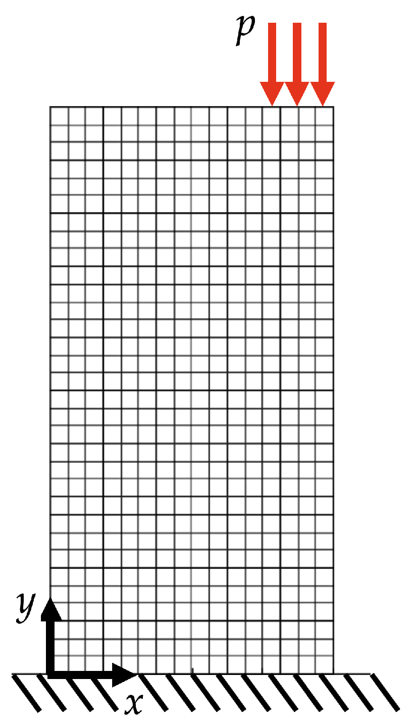
In the following, for all the six configurations depicted in Figure 6, an elastic problem is solved via the finite element method. A square panel of side is considered and subjected to a top pressure on a limited area with a resulting equivalent concentrated force of pointing downwards. The panel is clamped at the bottom. The problem is symmetrical for geometry and loads so only half of the domain is investigated. A regular squared finite element mesh of Q4 elements is considered and depicted in Figure 7.
The results are reported according to the contour plots of displacements, (horizontal) and (vertical), stresses, (horizontal), (vertical), relative rotation and shear strains and are shown.
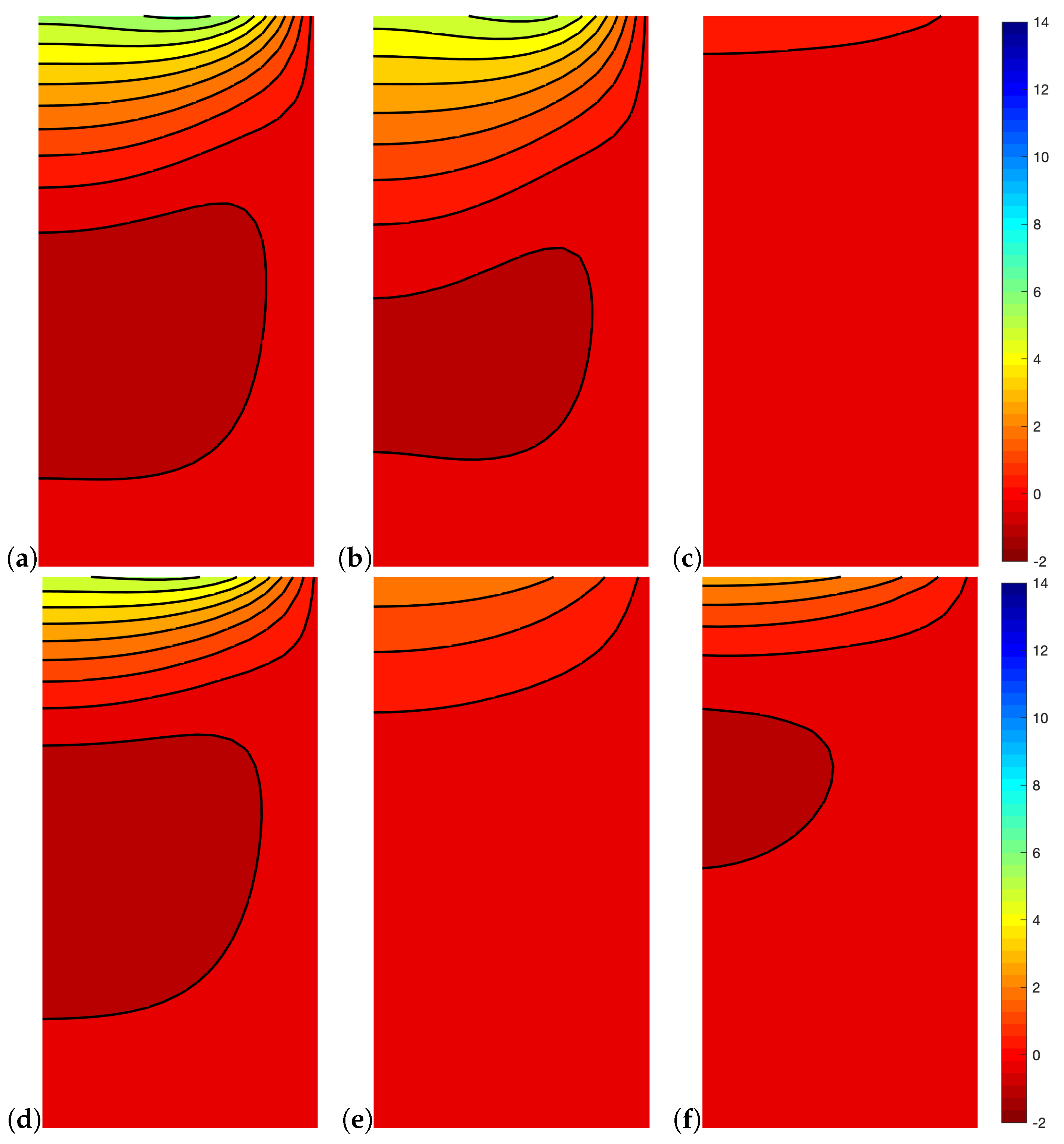
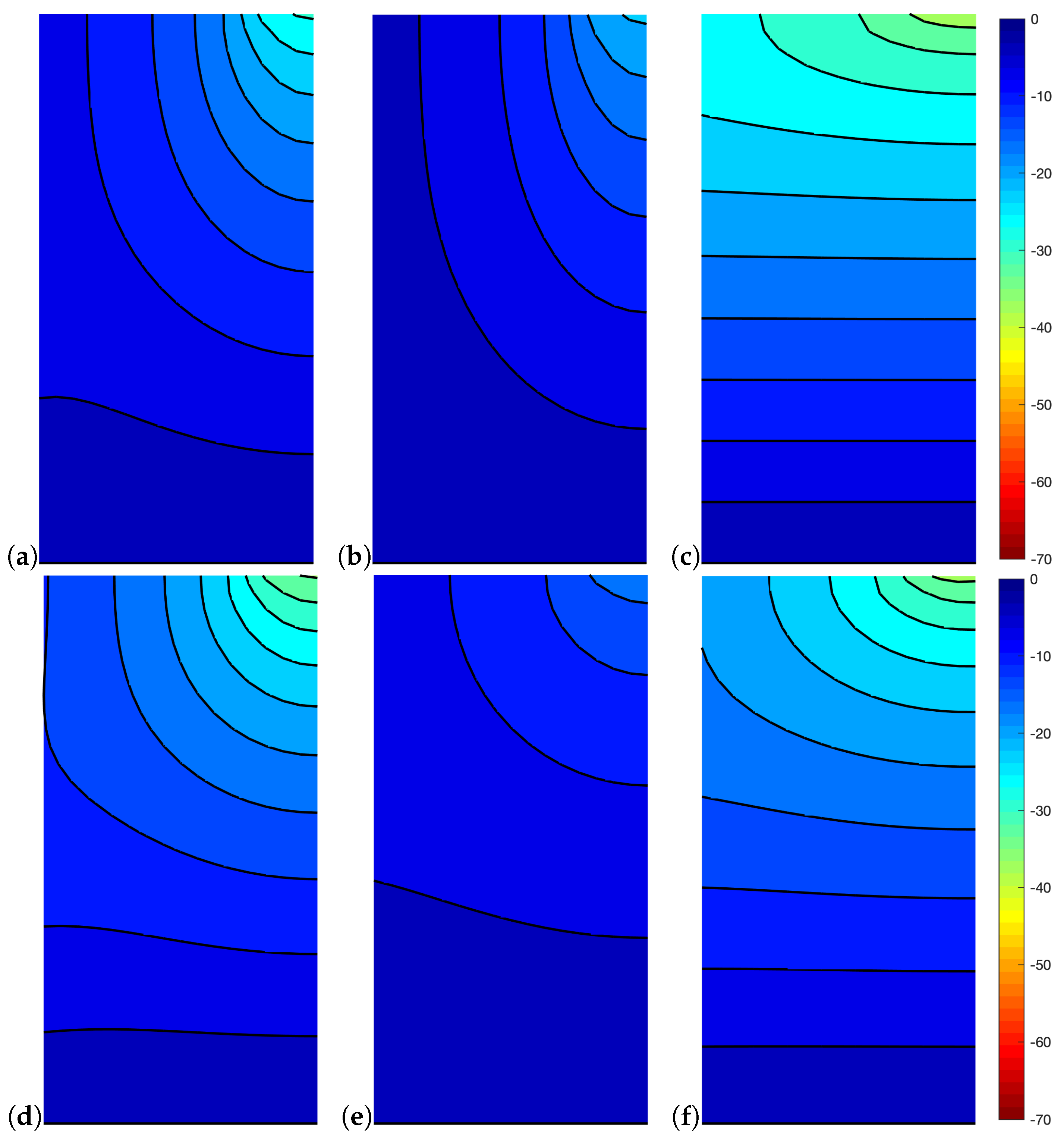
Horizontal displacement is depicted in Figure 8. It is evident that rectangular and regular hexagons correspond to orthotropic and orthotetragonal behaviors which in this case are very similar; the only difference between these two configuration is that orthotropic configuration has no Poisson effect. The hourglass configuration, which is auxetic (Poisson negative), has a stronger contraction of the material (larger horizontal displacement) close to the applied load as it is expected from auxetic materials. The other configurations that have all horizontally elongated tiles display very small horizontal motions, either positive or negative.
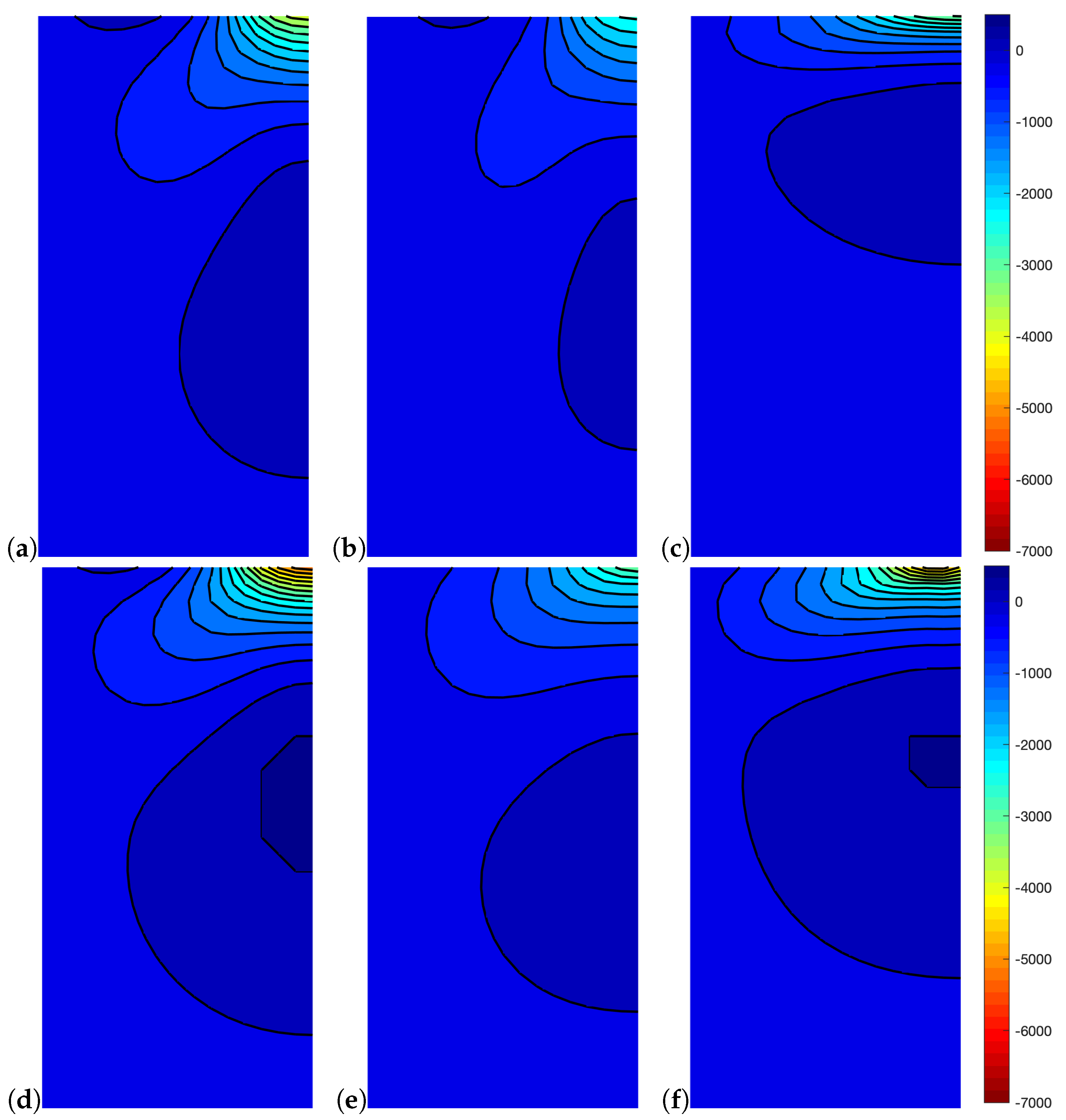
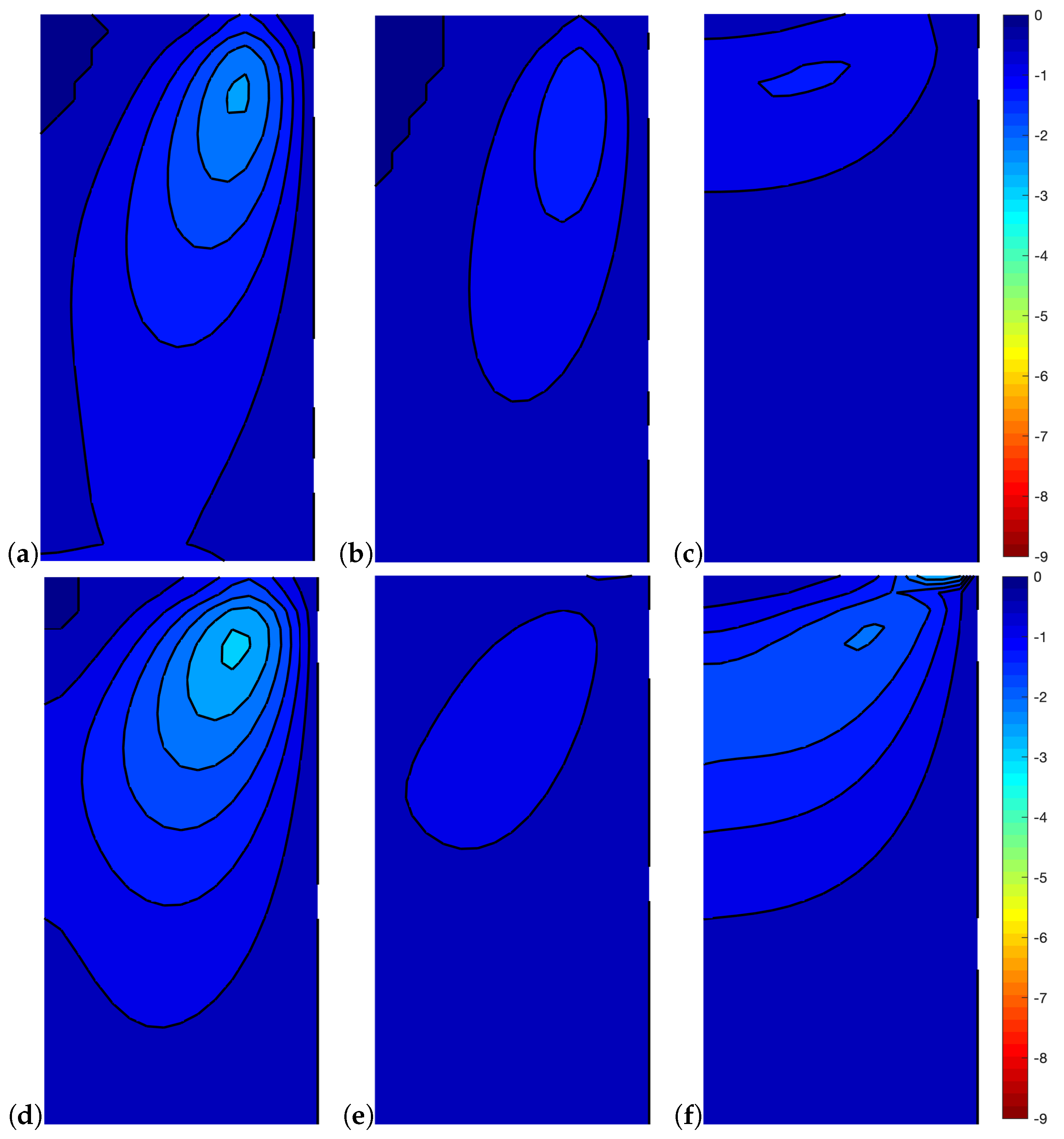
Vertical displacement is depicted in Figure 9. Rectangular and regular hexagons also have a similar behavior (except for the Poisson effect). The effect of negative Poisson ratio is visible in the hourglass configuration which displays concentrated vertical displacements and is close to zero displacements far from the applied load. This is due to the horizontal contraction of the material. Diamond and tip configurations, one not-chiral and one chiral, respectively, show similar behavior due to the horizontally elongated tiles. On the contrary, the smallest vertical displacements are measured for the skew configuration due to the engagement of tiles.
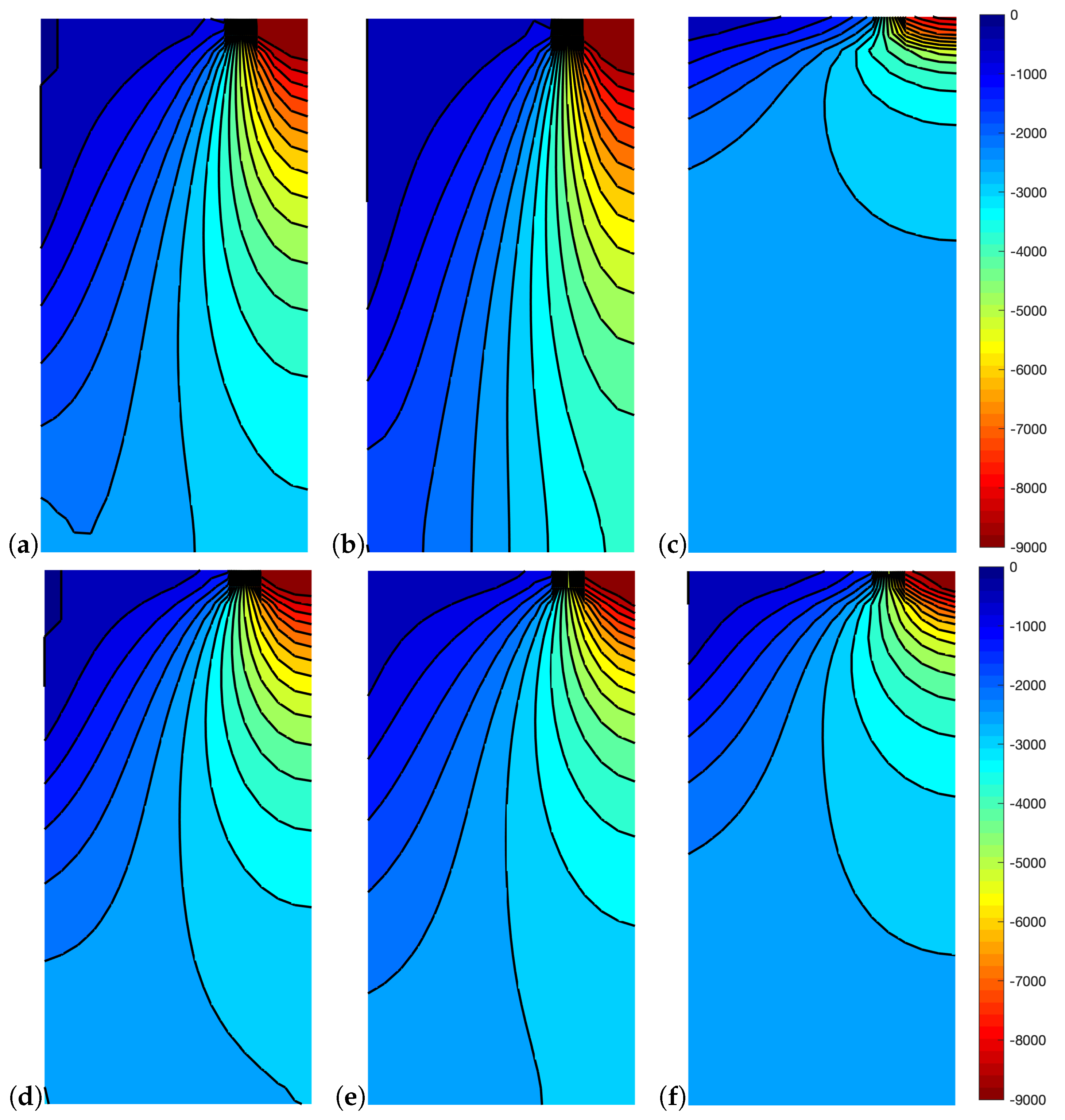
The horizontal stress is shown in Figure 10 does not reflect the map given by the horizontal displacement (Figure 8) due to the coupling between classical and micropolar quantities in the skew and tip configurations. In fact, the diamond configuration which registers small horizontal displacements has very localized horizontal stresses. Rectangular, auxetic and regular configurations have behaviors expected and already shown in [60]. Note that tip configuration, to which corresponds a small horizontal displacement, has a high and localized horizontal stress wherein the maximum value of the stress does not lay upon the symmetry axis as in all the other configurations. This translation of the maximum horizontal stress is due to the coupling between the horizontal stress and the curvature due to .
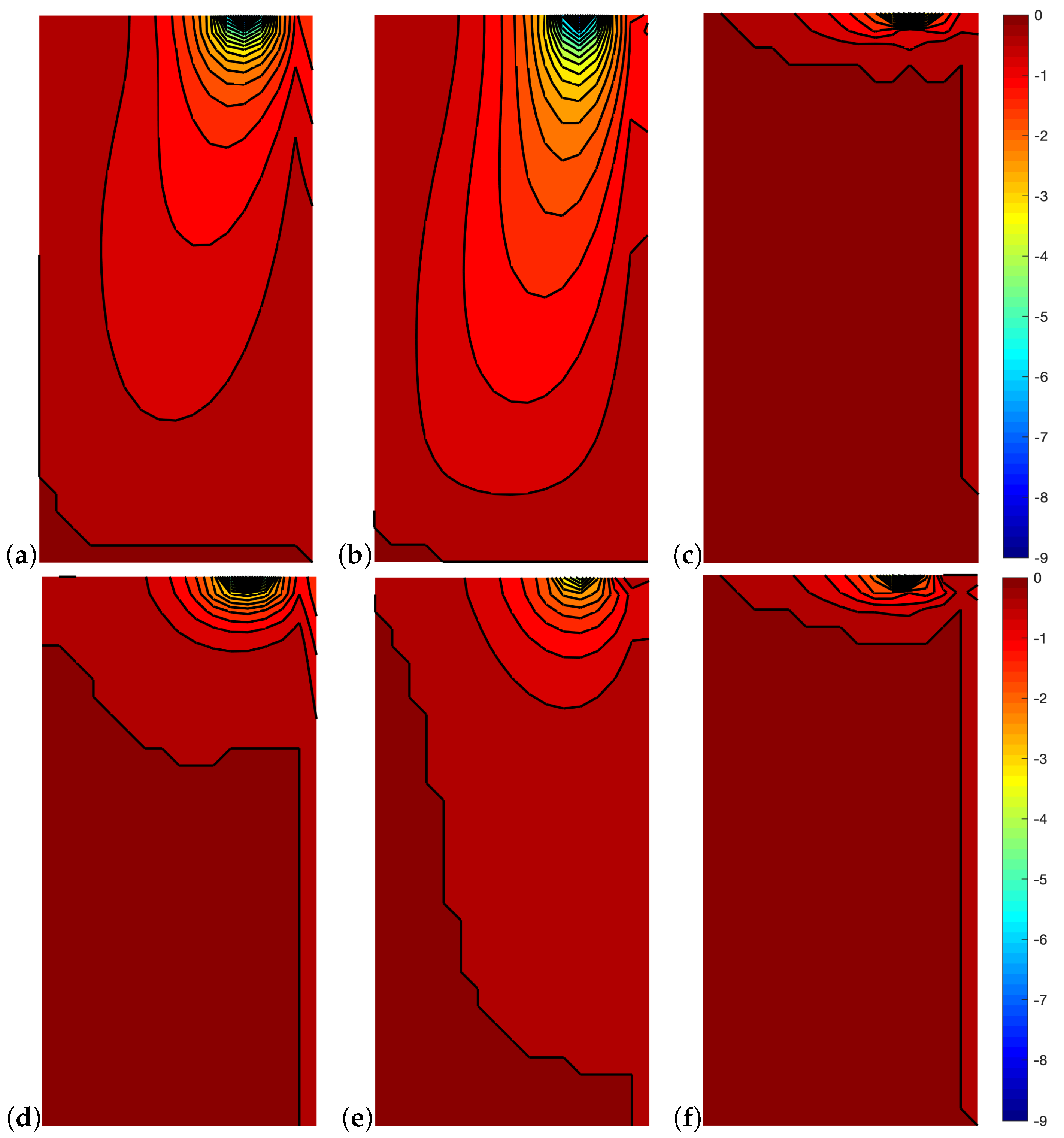
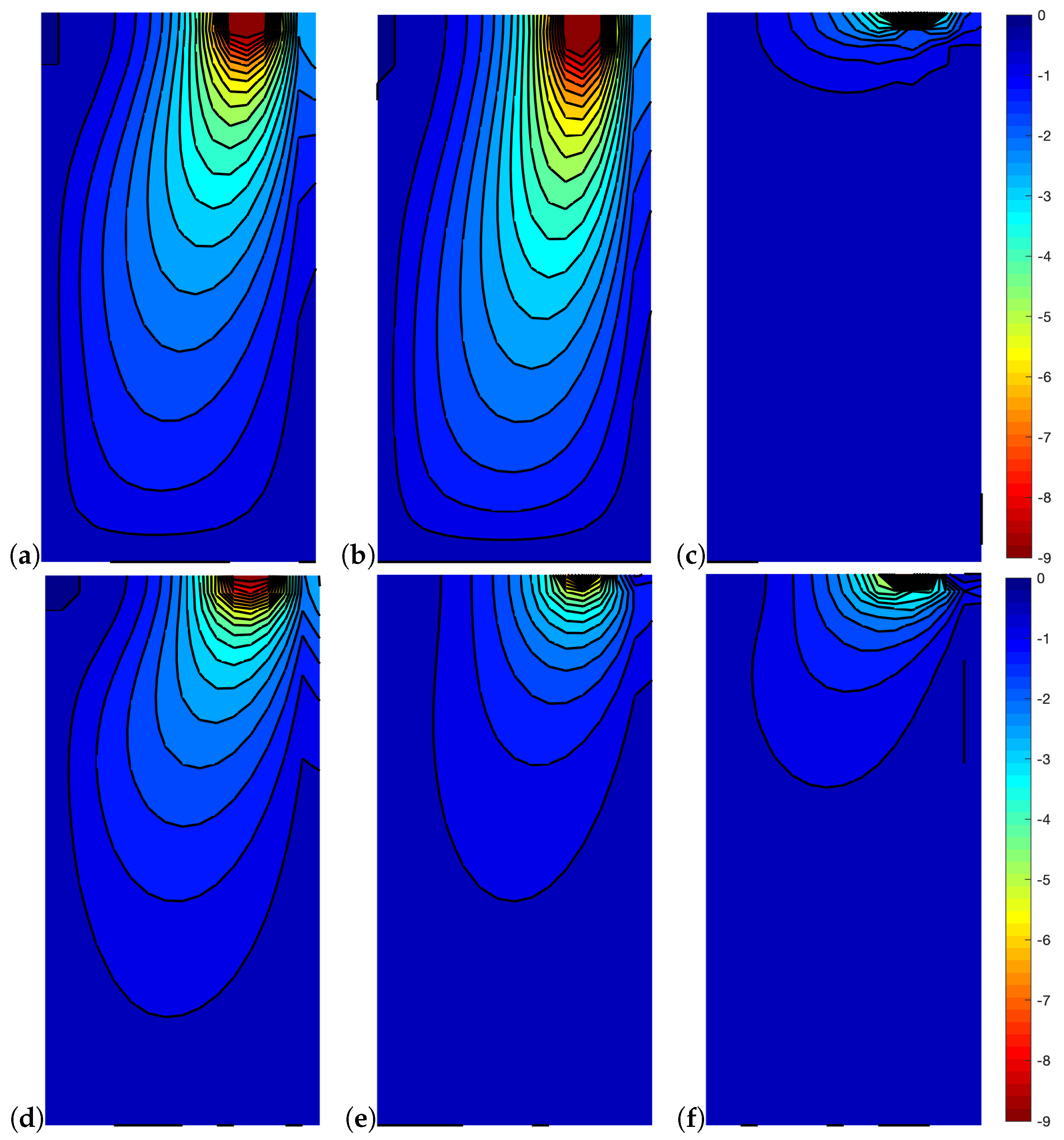
Vertical stress is shown in Figure 11. Stress percolation due to micropolar effect is shown by rectangular, auxetic, regular and skew configurations. Diamond and tip configurations display highly concentrated vertical stresses with stress fields that are negligible and close to the bottom boundary condition. The more evident stress percolation is observed in the hourglass configuration due to the higher ratio with respect to the others. The diamond configuration which has the smallest ratio observes a higher vertical stress concentration close to the applied load.
Similar to what has been observed in the previous works [50,60], the relative rotation, represented in Figure 12 is affected by not symmetric classical stiffnesses , chiral behavior and micropolar stiffnesses , . As an example, the rectangular configuration, which has an orthotropic behavior, shows a higher relative rotation than the skew and tip configurations, which are chiral. The same can be said if the rectangular configuration is compared to the regular one, which is orthotetragonal, and results in having a smaller relative rotation. As for the vertical stress case, once again, the hourglass configuration has the more evident relative rotation and on the contrary, the diamond configuration has almost zero relative rotation.
In the following unsymmetrical shear strains, and are discussed and displayed in Figure 13 and Figure 14. Classical behavior should be retrieved if ; in other words, no micropolar effect should be observed. and include
Although with some (in some cases small) variations, a micropolar effect is always observed for all configurations due to the fact that in all cases and also and for some cases. As expected, the configurations that observed a relative rotation close to zero in most of the solid (diamond, skew and tip) have that is a classical continuum. At the same time, the highest micropolar effect is observed in the auxetic behavior which had the largest variation of the relative rotation contour plot.
5. Conclusions
This paper investigated the static behavior of materials with hexagonal microstructures. A homogenization approach is applied to selected lattice assemblies in order to obtain a micropolar constitutive relation which results to be a function of two geometric parameters. Up to twelve nonzero elastic constants have been activated with the present procedure and the particular behavior of six material configurations (termed rectangular, auxetic, diamond, regular, skew and tip) have been presented. The selected patterns correspond to the so-called orthotropic, orthotetragonal, auxetic and chiral material symmetries. In particular, chirality occurs when asymmetric tiles are selected and an auxetic solid is derived when rehentrant corners are used.
Different levels of nonlocality, that in the case of micropolar media are of the ’implicit’ type, that are related to the geometric configuration, have been observed to be due to the bending moduli ratio, ratio, and to chiral terms (). However, chiral materials did not show the larger degree of micropolarity given by the auxetic configuration. None of the configurations correspond to classical continua, because no configuration has zero micropolar terms; however, the so-called diamond and tip configurations result in the ones with largest contour areas of zero relative rotation, that is, areas with strain that is quite symmetric, and then behave in a way that is similar to a classic material. Future developments of this work will be oriented to wider investigations of the effect of the relative rotations with a reliable measure of nonlocality.
Author Contributions
Conceptualization, N.F. and P.T.; methodology, P.T.; software, N.F.; validation, N.F., P.T.; formal analysis, N.F.; investigation, N.F.; resources, N.F., P.T. and R.L.; data curation, N.F.; writing–original draft preparation, N.F.; writing–review and editing, N.F., P.T. and R.L.; visualization, P.T. and R.L.; supervision, P.T.; project administration, P.T.; funding acquisition, P.T. All authors have read and agreed to the published version of the manuscript.
Funding
This research was supported by the Italian Ministry of University and Research, P.R.I.N. 2017 No. 20172017HFPKZY (cup: B86J16002300001).
Conflicts of Interest
The authors declare no conflict of interest.
References
- Baraldi, D.; Reccia, E.; Cecchi, A. In plane loaded masonry walls: DEM and FEM/DEM models. A critical review. Meccanica 2018, 53, 1613–1628. [Google Scholar] [CrossRef] [Green Version]
- Reccia, E.; Leonetti, L.; Trovalusci, P.; Cecchi, A. A multiscale/multidomain model for the failure analysis of masonry walls: A validation with a combined FEM/DEM approach. Int. J. Multiscale Comp. Eng. 2018, 16, 325–343. [Google Scholar] [CrossRef]
- Ehlers, W.; Ramm, E.; Diebels, S.; D’Addetta, G. From particle ensembles to Cosserat continua: Homogenization of contact forces towards stresses and couple stresses. Int. J. Solids Struct. 2003, 40, 6681–6702. [Google Scholar] [CrossRef]
- Bigoni, D.; Drugan, W.J. Analytical derivation of Cosserat moduli via homogenization of heterogeneous elastic materials. J. Appl. Mech. 2006, 74, 741–753. [Google Scholar] [CrossRef]
- Li, X.; Liu, Q.; Zhang, J. A micro–macro homogenization approach for discrete particle assembly—Cosserat continuum modeling of granular materials. Int. J. Solids Struct. 2010, 47, 291–303. [Google Scholar] [CrossRef]
- Reasa, D.R.; Lakes, R.S. Cosserat effects in achiral and chiral cubic lattices. J. Appl. Mech. 2019, 86, 111009. [Google Scholar] [CrossRef]
- Trovalusci, P. Molecular Approaches for Multifield Continua: Origins and current developments. In Multiscale Modeling of Complex Materials: Phenomenological, Theoretical and Computational Aspects; Sadowski, T., Trovalusci, P., Eds.; Springer: Vienna, Austria, 2014; pp. 211–278. [Google Scholar]
- Tuna, M.; Kirca, M.; Trovalusci, P. Deformation of atomic models and their equivalent continuum counterparts using Eringen’s two-phase local/nonlocal model. Mech. Res. Commun. 2019, 97, 26–32. [Google Scholar] [CrossRef] [Green Version]
- Tuna, M.; Trovalusci, P. Scale dependent continuum approaches for discontinuous assemblies: ‘Explicit’ and ‘implicit’ non-local models. Mech. Res. Commun. 2020, 103, 103461. [Google Scholar] [CrossRef]
- Larsson, R.; Zhang, Y. Homogenization of microsystem interconnects based on micropolar theory and discontinuous kinematics. J. Mech. Phys. Solids 2007, 55, 819–841. [Google Scholar] [CrossRef]
- Alibert, J.J.; Della Corte, A. Second-gradient continua as homogenized limit of pantographic microstructured plates: A rigorous proof. Z. Für Angew. Math. Und Phys. 2015, 66, 2855–2870. [Google Scholar] [CrossRef]
- Demir, C.; Civalek, O. On the analysis of microbeams. Int. J. Eng. Sci. 2017, 121, 14–33. [Google Scholar] [CrossRef]
- Civalek, O.; Demir, C. A simple mathematical model of microtubules surrounded by an elastic matrix by nonlocal finite element method. Appl. Math. Comput. 2016, 289, 335–352. [Google Scholar] [CrossRef]
- Sluys, L.; de Borst, R.; Muhlhaus, H.B. Wave propagation, localization and dispersion in a gradient-dependent medium. Int. J. Solids Struct. 1993, 30, 1153–1171. [Google Scholar] [CrossRef] [Green Version]
- Kouznetsova, V.; Geers, M.G.D.; Brekelmans, W.A.M. Multi-scale constitutive modelling of heterogeneous materials with a gradient-enhanced computational homogenization scheme. Int. J. Numer. Methods Eng. 2002, 54, 1235–1260. [Google Scholar] [CrossRef]
- Kouznetsova, V.; Geers, M.; Brekelmans, W. Multi-scale second-order computational homogenization of multi-phase materials: A nested finite element solution strategy. Comput. Methods Appl. Mech. Eng. 2004, 193, 5525–5550. [Google Scholar] [CrossRef]
- Massart, T.J.; Peerlings, R.H.J.; Geers, M.G.D. An enhanced multi-scale approach for masonry wall computations with localization of damage. Int. J. Numer. Methods Eng. 2007, 69, 1022–1059. [Google Scholar] [CrossRef] [Green Version]
- Capecchi, D.; Ruta, G.; Trovalusci, P. Voigt and Poincaré’s mechanistic–energetic approaches to linear elasticity and suggestions for multiscale modelling. Arch. Appl. Mech. 2011, 81, 1573–1584. [Google Scholar] [CrossRef]
- Leismann, T.; Mahnken, R. Comparison of hyperelastic micromorphic, micropolar and microstrain continua. Int. J. Non-Linear Mech. 2015, 77, 115–127. [Google Scholar] [CrossRef]
- Peerlings, R.H.J.; Fleck, N.A. Computational evaluation of strain gradient elasticity constants. Int. J. Multiscale Comput. Eng. 2004, 2. [Google Scholar] [CrossRef]
- Uzun, B.; Civalek, O. Nonlocal FEM formulation for vibration analysis of nanowires on elastic matrix with different materials. Math. Comput. Appl. 2019, 24, 38. [Google Scholar] [CrossRef] [Green Version]
- Drugan, W.; Willis, J. A micromechanics-based nonlocal constitutive equation and estimates of representative volume element size for elastic composites. J. Mech. Phys. Solids 1996, 44, 497–524. [Google Scholar] [CrossRef]
- Luciano, R.; Willis, J. Bounds on non-local effective relations for random composites loaded by configuration-dependent body force. J. Mech. Phys. Solids 2000, 48, 1827–1849. [Google Scholar] [CrossRef]
- Smyshlyaev, V.; Cherednichenko, K. On rigorous derivation of strain gradient effects in the overall behaviour of periodic heterogeneous media. J. Mech. Phys. Solids 2000, 48, 1325–1357. [Google Scholar] [CrossRef]
- Bacca, M.; Bigoni, D.; Corso, F.D.; Veber, D. Mindlin second-gradient elastic properties from dilute two-phase Cauchy-elastic composites. Part I: Closed form expression for the effective higher-order constitutive tensor. Int. J. Solids Struct. 2013, 50, 4010–4019. [Google Scholar] [CrossRef] [Green Version]
- Barretta, R.; Luciano, R.; de Sciarra, F.M. A fully gradient model for Euler-Bernoulli nanobeams. Math. Probl. Eng. 2015, 2015. [Google Scholar] [CrossRef] [Green Version]
- Demir, C.; Civalek, O. A new nonlocal FEM via Hermitian cubic shape functions for thermal vibration of nano beams surrounded by an elastic matrix. Compos. Struct. 2017, 168, 872–884. [Google Scholar] [CrossRef]
- Canadija, M.; Barretta, R.; de Sciarra, F.M. A gradient elasticity model of Bernoulli-Euler nanobeams in non-isothermal environments. Eur. J. Mech. A Solids 2016, 55, 243–255. [Google Scholar] [CrossRef]
- Barretta, R.; de Sciarra, F.M. A nonlocal model for carbon nanotubes under axial loads. Adv. Mater. Sci. Eng. 2013, 2013. [Google Scholar] [CrossRef] [Green Version]
- Barretta, R.; Faghidian, S.A.; Luciano, R. Longitudinal vibrations of nano-rods by stress-driven integral elasticity. Mech. Adv. Mater. Struct. 2019, 26, 1307–1315. [Google Scholar] [CrossRef]
- Masiani, R.; Trovalusci, P. Cosserat and Cauchy materials as continuum models of brick masonry. Meccanica 1996, 31, 421–432. [Google Scholar] [CrossRef]
- Forest, S.; Sab, K. Cosserat overall modeling of heterogeneous materials. Mech. Res. Commun. 1998, 25, 449–454. [Google Scholar] [CrossRef]
- Forest, S.; Dendievel, R.; Canova, G.R. Estimating the overall properties of heterogeneous Cosserat materials. Model. Simul. Mater. Sci. Eng. 1999, 7, 829–840. [Google Scholar] [CrossRef]
- Ostoja-Starzewski, M.; Boccara, S.D.; Jasiuk, I. Couple-stress moduli and characteristics length of a two-phase composite. Mech. Res. Commun. 1999, 26, 387–396. [Google Scholar] [CrossRef]
- Bouyge, F.; Jasiuk, I.; Ostoja-Starzewski, M. A micromechanically based couple–stress model of an elastic two-phase composite. Int. J. Solids Struct. 2001, 38, 1721–1735. [Google Scholar] [CrossRef]
- Forest, S.; Pradel, F.; Sab, K. Asymptotic analysis of heterogeneous Cosserat media. Int. J. Solids Struct. 2001, 38, 4585–4608. [Google Scholar] [CrossRef]
- Onck, P.R. Cosserat modeling of cellular solids. Comptes Rendus MÉcanique 2002, 330, 717–722. [Google Scholar] [CrossRef]
- Trovalusci, P.; Masiani, R. Non-linear micropolar and classical continua for anisotropic discontinuous materials. Int. J. Solids Struct. 2003, 40, 1281–1297. [Google Scholar] [CrossRef]
- Trovalusci, P.; Masiani, R. A multifield model for blocky materials based on multiscale description. Int. J. Solids Struct. 2005, 42, 5778–5794. [Google Scholar] [CrossRef] [Green Version]
- Trovalusci, P.; Sansalone, V. A Numerical Investigation of Structure-Property Relations in Fiber Composite Materials. Int. J. Multiscale Comput. Eng. 2007, 5, 141–152. [Google Scholar]
- Tekoglu, C.; Onck, P.R. Size effects in two-dimensional Voronoi foams: A comparison between generalized continua and discrete models. J. Mech. Phys. Solids 2008, 56, 3541–3564. [Google Scholar] [CrossRef]
- Kunin, I.A. The theory of elastic media with microstructure and the theory of dislocations. In Mechanics of Generalized Continua; Kröner, E., Ed.; Springer: Berlin/Heidelberg, Germany, 1968; pp. 321–329. [Google Scholar]
- Trovalusci, P.; Varano, V.; Rega, G. A generalized continuum formulation for composite microcracked materials and wave propagation in a bar. J. Appl. Mech. 2010, 77, 061002. [Google Scholar] [CrossRef]
- Reda, H.; Rahali, Y.; Ganghoffer, J.; Lakiss, H. Wave propagation in 3D viscoelastic auxetic and textile materials by homogenized continuum micropolar models. Compos. Struct. 2016, 141, 328–345. [Google Scholar] [CrossRef]
- Eremeyev, V.A.; Rosi, G.; Naili, S. Transverse surface waves on a cylindrical surface with coating. Int. J. Eng. Sci. 2019, 147, 103188. [Google Scholar] [CrossRef]
- Settimi, V.; Trovalusci, P.; Rega, G. Dynamical properties of a composite microcracked bar based on a generalized continuum formulation. Contin. Mech. Thermodyn. 2019, 31, 1627–1644. [Google Scholar] [CrossRef] [Green Version]
- Trovalusci, P.; Masiani, R. Material symmetries of micropolar continua equivalent to lattices. Int. J. Solids Struct. 1999, 36, 2091–2108. [Google Scholar] [CrossRef]
- Pau, A.; Trovalusci, P. Block masonry as equivalent micropolar continua: The role of relative rotations. Acta Mech. 2012, 223, 1455–1471. [Google Scholar] [CrossRef]
- Trovalusci, P.; Pau, A. Derivation of microstructured continua from lattice systems via principle of virtual works: The case of masonry-like materials as micropolar, second gradient and classical continua. Acta Mech. 2014, 225, 157–177. [Google Scholar] [CrossRef]
- Fantuzzi, N.; Trovalusci, P.; Dharasura, S. Mechanical behavior of anisotropic composite materials as micropolar continua. Front. Mater. 2019, 6, 59. [Google Scholar] [CrossRef]
- Chen, W.; Xu, M.; Li, L. A model of composite laminated Reddy plate based on new modified couple stress theory. Compos. Struct. 2012, 94, 2143–2156. [Google Scholar] [CrossRef]
- Roque, C.; Fidalgo, D.; Ferreira, A.; Reddy, J. A study of a microstructure-dependent composite laminated Timoshenko beam using a modified couple stress theory and a meshless method. Compos. Struct. 2013, 96, 532–537. [Google Scholar] [CrossRef]
- Fantuzzi, N.; Leonetti, L.; Trovalusci, P.; Tornabene, F. Some novel numerical applications of Cosserat continua. Int. J. Comput. Methods 2018, 15, 1850054. [Google Scholar] [CrossRef]
- Trovalusci, P.; Bellis, M.L.D.; Masiani, R. A multiscale description of particle composites: From lattice microstructures to micropolar continua. Compos. Part B Eng. 2017, 128, 164–173. [Google Scholar] [CrossRef] [Green Version]
- Rizzi, G.; Corso, F.D.; Veber, D.; Bigoni, D. Identification of second-gradient elastic materials from planar hexagonal lattices. Part II: Mechanical characteristics and model validation. Int. J. Solids Struct. 2019, 176–177, 19–35. [Google Scholar] [CrossRef] [Green Version]
- Eremeyev, V.A.; Pietraszkiewicz, W. Material symmetry group and constitutive equations of micropolar anisotropic elastic solids. Math. Mech. Solids 2016, 21, 210–221. [Google Scholar] [CrossRef]
- Aguiar, A.R.; Lopes da Rocha, G. On the number of invariants in the strain energy density of an anisotropic nonlinear elastic material with Two Material Symmetry Directions. J. Elast. 2018, 131, 125–132. [Google Scholar] [CrossRef]
- Scherphuis, J. Jaap’s Puzzle Page. 2019. Available online: http://www.jaapsch.net/tilings (accessed on 19 September 2019).
- Sokolowski, M. Theory of Couple–Stresses in Bodies with Constrained Rotations; CISM Courses and Lectures; Springer: Vienna, Austria, 1972. [Google Scholar]
- Fantuzzi, N.; Trovalusci, P.; Luciano, R. Multiscale analysis of anisotropic materials with hexagonal microstructure as micro-polar continua. Int. J. Multiscale Comput. Eng. 2020, 1, 1–20. [Google Scholar]
- Leonetti, L.; Fantuzzi, N.; Trovalusci, P.; Tornabene, F. Scale effects in orthotropic composite assemblies as micropolar continua: A comparison between weak- and strong-form finite element solutions. Materials 2019, 12, 758. [Google Scholar] [CrossRef] [Green Version]
- Ferreira, A. MATLAB Codes for Finite Element Analysis: Solids and Structures. In Solid Mechanics and Its Applications; Springer: Amsterdam, The Netherlands, 2008. [Google Scholar]
Figure 1.
Present hexagonal pattern and single tile geometry.

Figure 2.
Possible configurations as a function of and for constant value of .

Figure 3.
Hexagonal patterns given : (a) rectangular , (b) hourglass , (c) diamond , (d) regular , (e) skew , (f) tip , .
Figure 3.
Hexagonal patterns given : (a) rectangular , (b) hourglass , (c) diamond , (d) regular , (e) skew , (f) tip , .

Figure 4.
Stress/strain elastic stiffness variation with : (a) , (b) , (c) , (d) , (e) , (f) .

Figure 5.
microcouple/strain elastic stiffness variation with : (a) , (b) , (c) , (d) , (e) , (f) .

Figure 6.
Hexagonal RVEs with geometric parameters and : (a) rectangular , (b) hourglass , (c) diamond , (d) regular , (e) skew , (f) tip , .
Figure 6.
Hexagonal RVEs with geometric parameters and : (a) rectangular , (b) hourglass , (c) diamond , (d) regular , (e) skew , (f) tip , .

Figure 7.
Current mesh used Q4 elements with displayed applied load and boundary conditions.

Figure 8.
Horizontal displacement for : (a) rectangular , (b) hourglass , (c) diamond , (d) regular , (e) skew , (f) tip , .
Figure 8.
Horizontal displacement for : (a) rectangular , (b) hourglass , (c) diamond , (d) regular , (e) skew , (f) tip , .

Figure 9.
Vertical displacement for : (a) rectangular , (b) hourglass , (c) diamond , (d) regular , (e) skew , (f) tip , .
Figure 9.
Vertical displacement for : (a) rectangular , (b) hourglass , (c) diamond , (d) regular , (e) skew , (f) tip , .

Figure 10.
Horizontal stress for : (a) rectangular , (b) hourglass , (c) diamond , (d) regular , (e) skew , (f) tip , .
Figure 10.
Horizontal stress for : (a) rectangular , (b) hourglass , (c) diamond , (d) regular , (e) skew , (f) tip , .

Figure 11.
Vertical stress for : (a) rectangular , (b) hourglass , (c) diamond , (d) regular , (e) skew , (f) tip , .
Figure 11.
Vertical stress for : (a) rectangular , (b) hourglass , (c) diamond , (d) regular , (e) skew , (f) tip , .

Figure 12.
Relative rotation for : (a) rectangular , (b) hourglass , (c) diamond , (d) regular , (e) skew , (f) tip , .
Figure 12.
Relative rotation for : (a) rectangular , (b) hourglass , (c) diamond , (d) regular , (e) skew , (f) tip , .

Figure 13.
Shear strain for : (a) rectangular , (b) hourglass , (c) diamond , (d) regular , (e) skew , (f) tip , .
Figure 13.
Shear strain for : (a) rectangular , (b) hourglass , (c) diamond , (d) regular , (e) skew , (f) tip , .

Figure 14.
Shear strain for : (a) rectangular , (b) hourglass , (c) diamond , (d) regular , (e) skew , (f) tip , .
Figure 14.
Shear strain for : (a) rectangular , (b) hourglass , (c) diamond , (d) regular , (e) skew , (f) tip , .


Table 1.
This is a table caption. Tables should be placed in the main text near to the first time they are cited.
Table 1.
This is a table caption. Tables should be placed in the main text near to the first time they are cited.
| Rect | Hour | Diam | Reg | Skew | Tip | |
|---|---|---|---|---|---|---|
| 287.3 | 209.2 | 2823 | 496.88 | 835.37 | 1123 | |
| 0 | −0.5 | 1.4894 | 0.79247 | 0 | 0.6714 | |
| 711.8 | 1059.7 | 333.57 | 496.88 | 1127.3 | 419.94 | |
| 710 | 1056.8 | 331.73 | 495.29 | 1121 | 418.1 | |
| 0 | −0.5 | 1.4894 | 0.79247 | 0 | 0.6714 | |
| 285.5 | 208.2 | 2836.9 | 495.29 | 839.47 | 1124.2 | |
| 0 | 0 | 0 | 0 | 0 | 30.03 | |
| 0 | 0 | 0 | 0 | −216.71 | −88.869 | |
| 0 | 0 | 0 | 0 | 0 | 30.03 | |
| 0 | 0 | 0 | 0 | 0 | −103.94 | |
| 14.4 | 11.9 | 1219.3 | 33.338 | 360.81 | 340.19 | |
| 44.2 | 67.7 | 89.941 | 33.338 | 303.95 | 79.488 |
© 2020 by the authors. Licensee MDPI, Basel, Switzerland. This article is an open access article distributed under the terms and conditions of the Creative Commons Attribution (CC BY) license (http://creativecommons.org/licenses/by/4.0/).
Share and Cite
MDPI and ACS Style
Fantuzzi, N.; Trovalusci, P.; Luciano, R. Material Symmetries in Homogenized Hexagonal-Shaped Composites as Cosserat Continua. Symmetry 2020, 12, 441. https://0-doi-org.brum.beds.ac.uk/10.3390/sym12030441
AMA Style
Fantuzzi N, Trovalusci P, Luciano R. Material Symmetries in Homogenized Hexagonal-Shaped Composites as Cosserat Continua. Symmetry. 2020; 12(3):441. https://0-doi-org.brum.beds.ac.uk/10.3390/sym12030441
Chicago/Turabian StyleFantuzzi, Nicholas, Patrizia Trovalusci, and Raimondo Luciano. 2020. "Material Symmetries in Homogenized Hexagonal-Shaped Composites as Cosserat Continua" Symmetry 12, no. 3: 441. https://0-doi-org.brum.beds.ac.uk/10.3390/sym12030441
Note that from the first issue of 2016, this journal uses article numbers instead of page numbers. See further details here.