Inertial Extra-Gradient Method for Solving a Family of Strongly Pseudomonotone Equilibrium Problems in Real Hilbert Spaces with Application in Variational Inequality Problem

 ,
,  ,
,  ,
,  and
and 
Abstract
:1. Introduction
2. Background
- (i).
- Strongly monotone if
- (ii).
- Monotone if
- (iii).
- Strongly pseudomonotone if
- (iv).
- Pseudomonotone if
- (v).
- Satisfying the Lipschitz-type condition on C if there are two positive real numbers such that
3. Convergence Analysis for an Algorithm
- f1.
- , for all and f is strongly pseudomonotone on .
- f2.
- f satisfy the Lipschitz-type condition through two positive constants and .
- f3.
- is convex and subdifferentiable on C for each fixed .
| Algorithm 1 (Inertial extragradient algorithm for strongly pseudomonotone equilibrium problems). |
|
- i.
- Let and computewhere be the sequence of positive real numbers satisfy the following conditions:
4. Application to Variational Inequality Problems
- strongly pseudomonotone upon C for if
- L-Lipschitz continuous upon C if
- G1.
- G is strongly pseudomonotone on C and ;
- G2.
- G is L-Lipschitz continuous upon C for some constant
- i.
- Choose and a sequence such thatholds. In addition, let be the sequence of positive real numbers which meets the following criteria:
- ii.
- Choose such that where
- iii.
- Compute
- i.
- Choose and computewhere be the sequence of positive real numbers satisfy the following conditions:
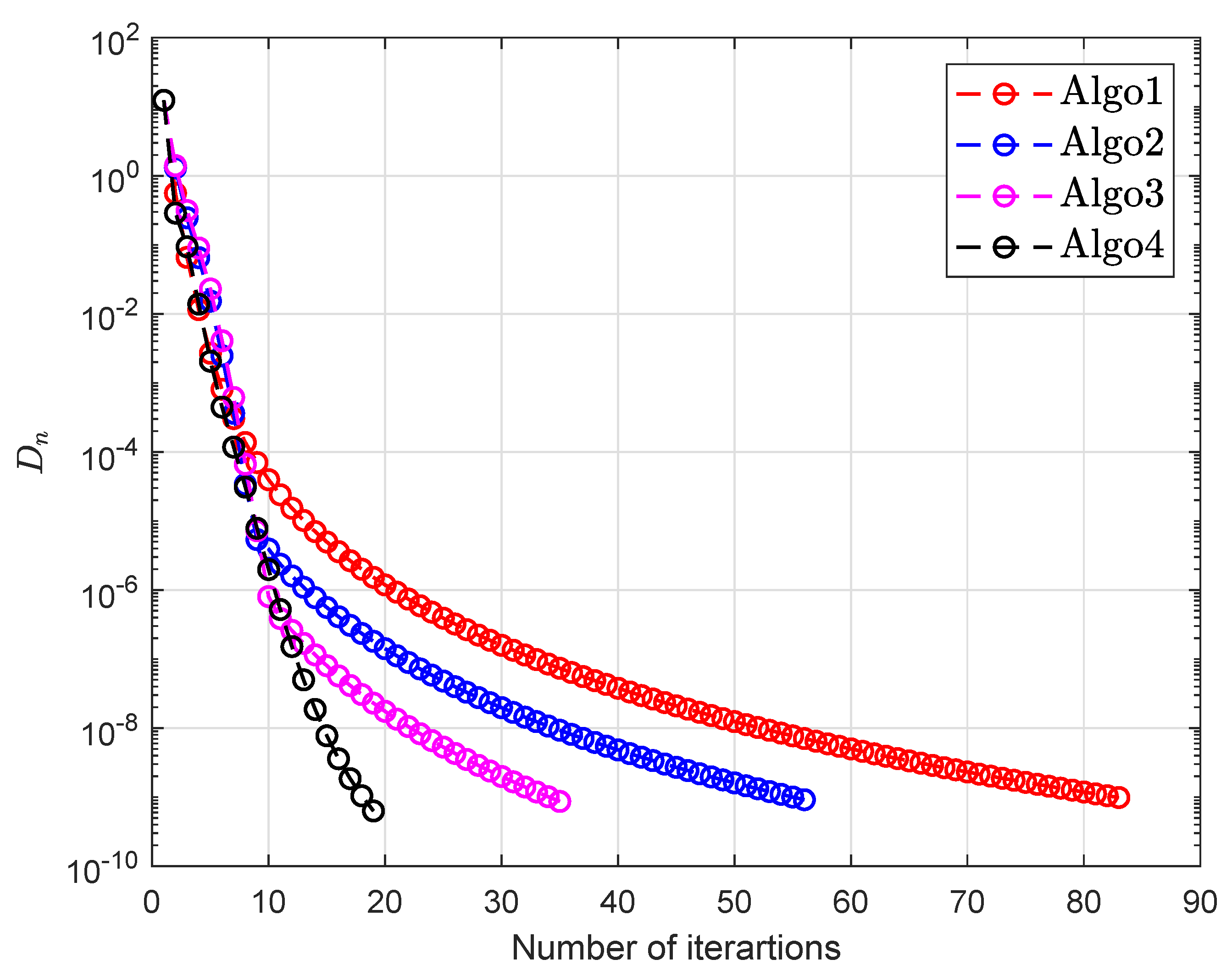
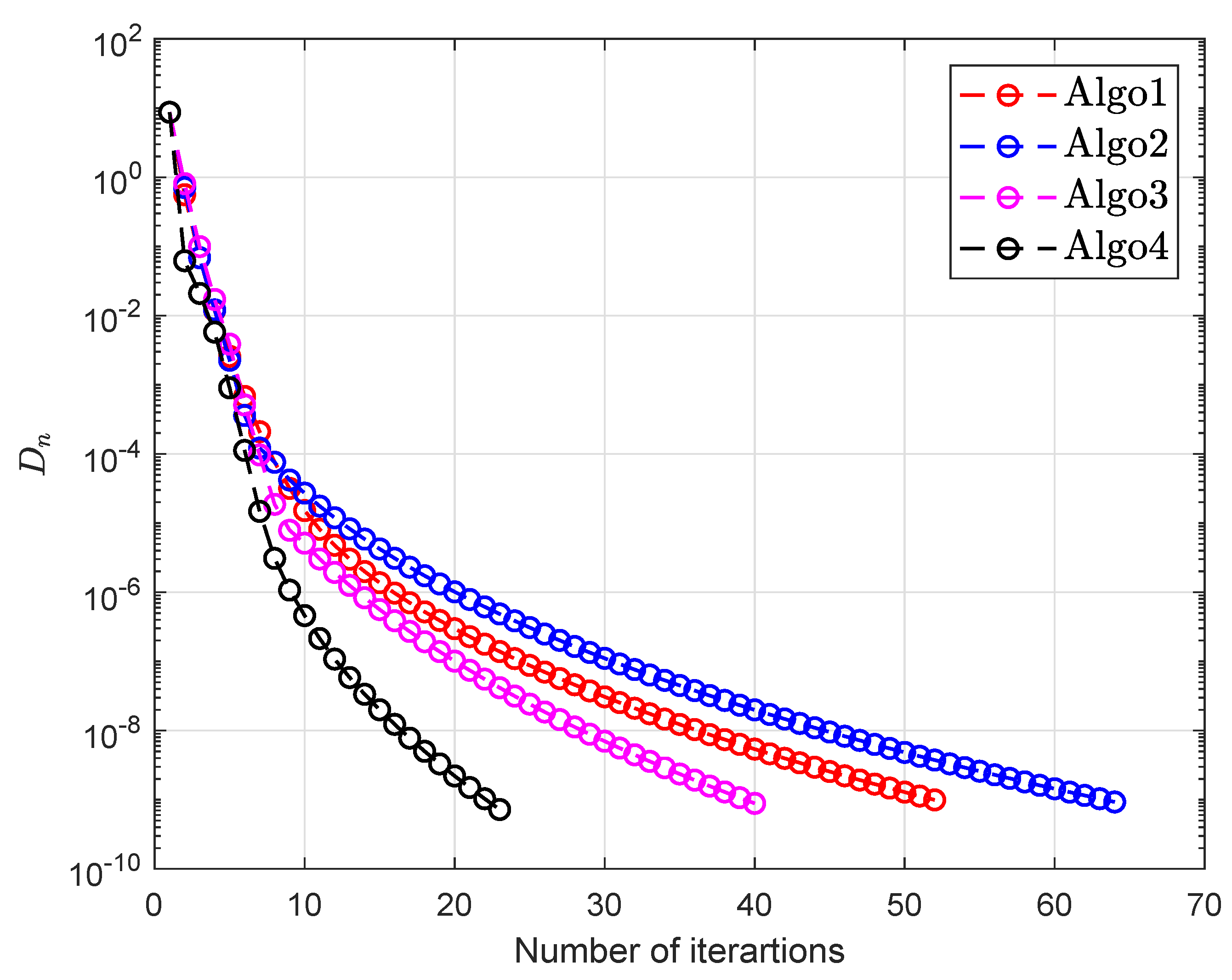
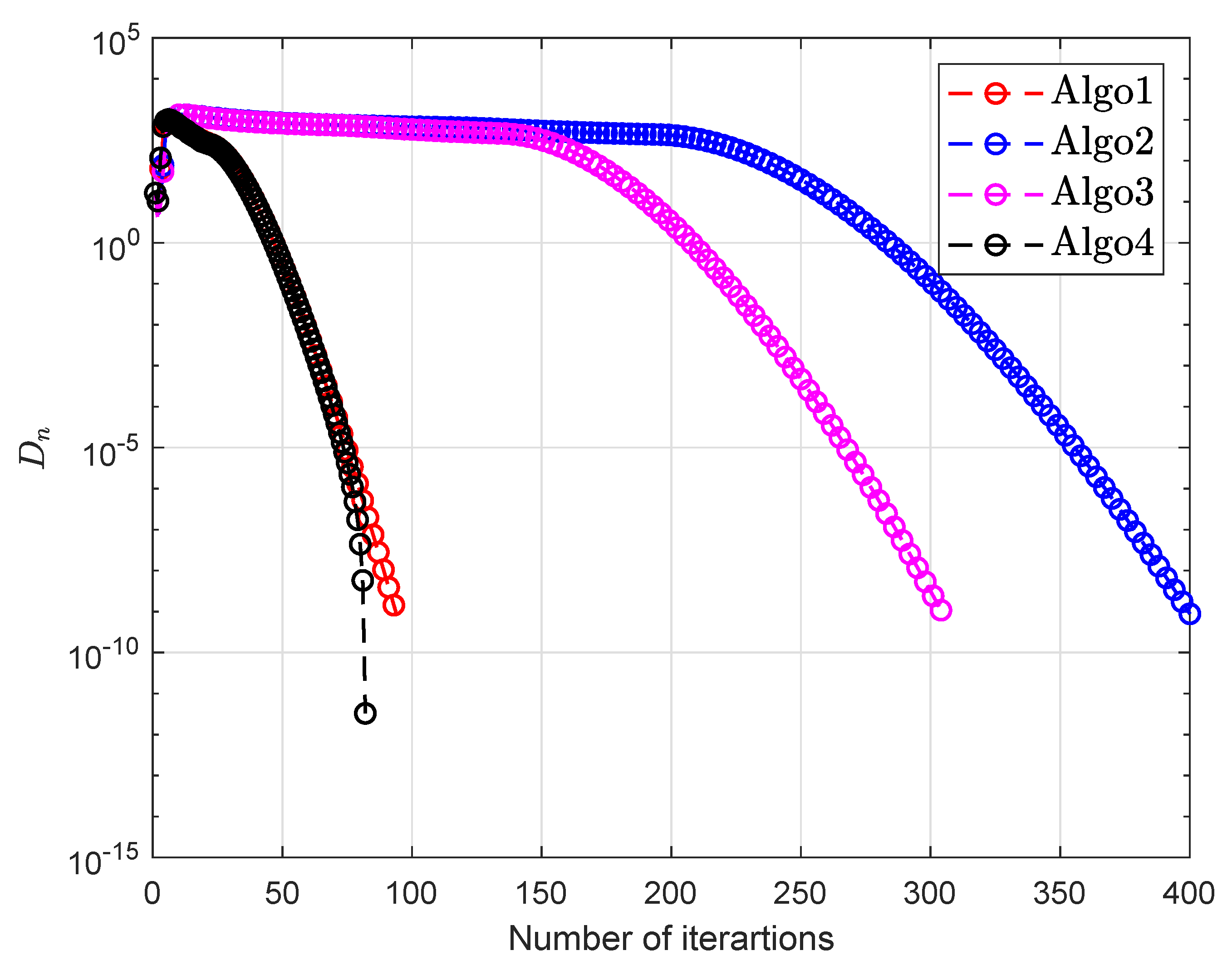
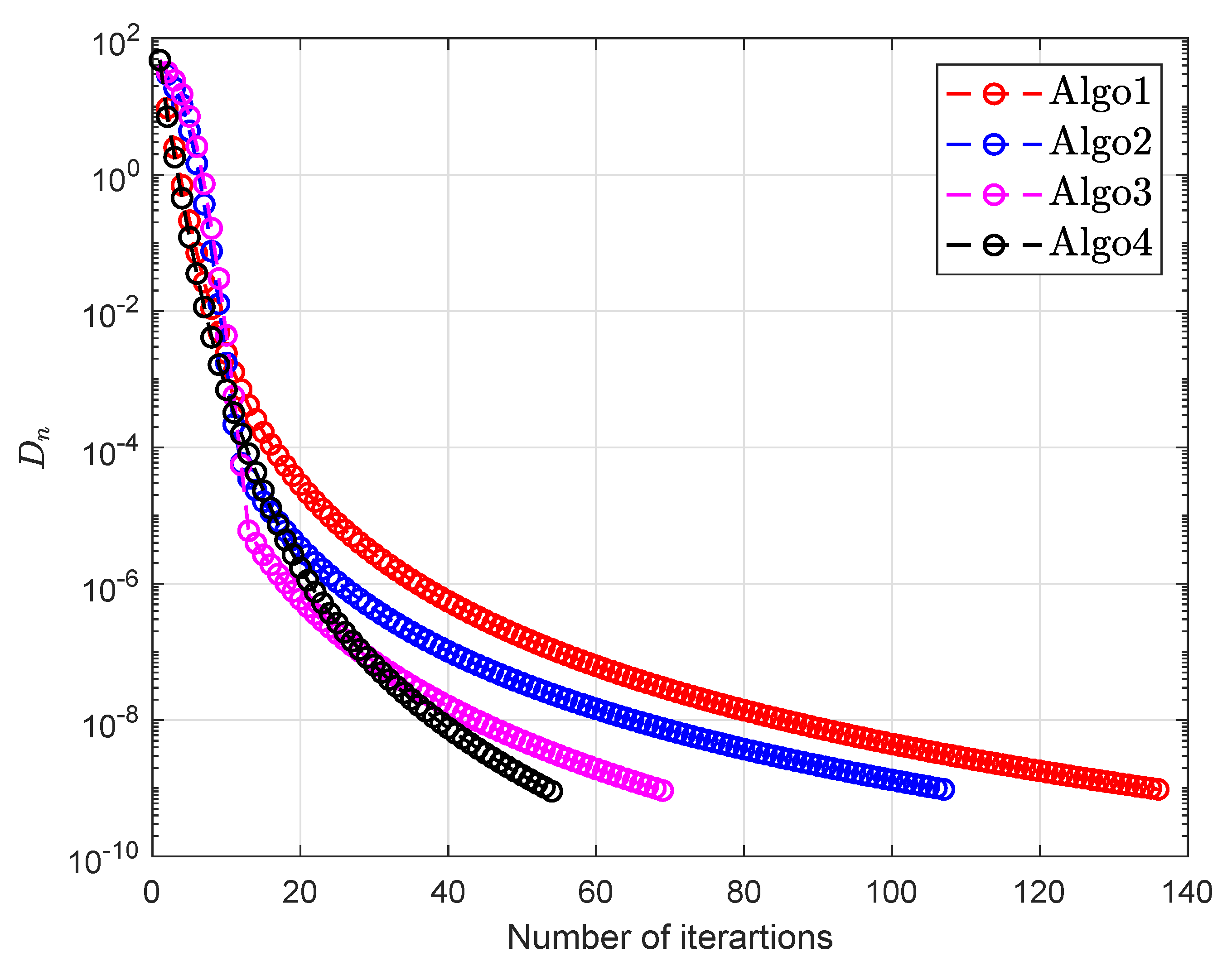
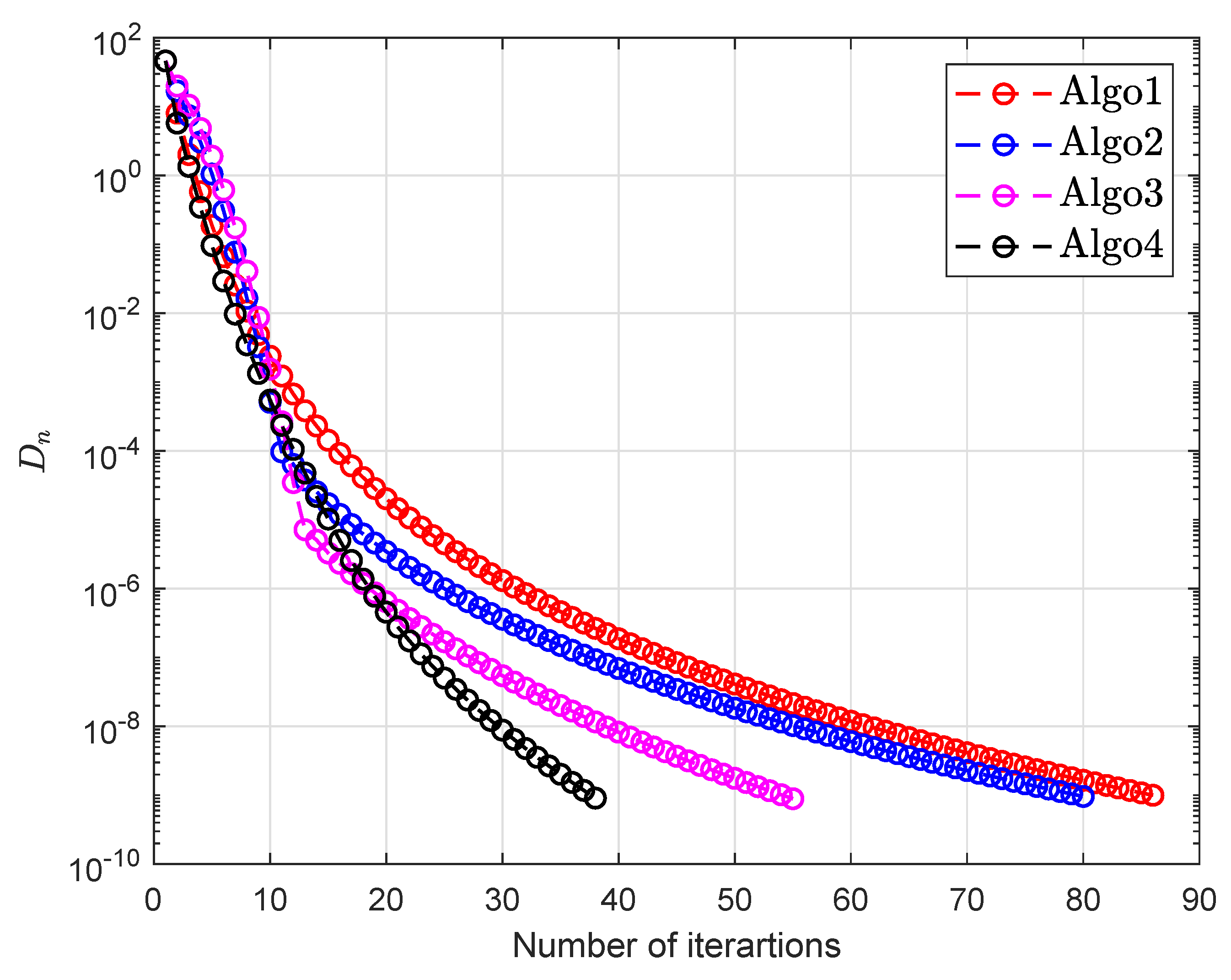
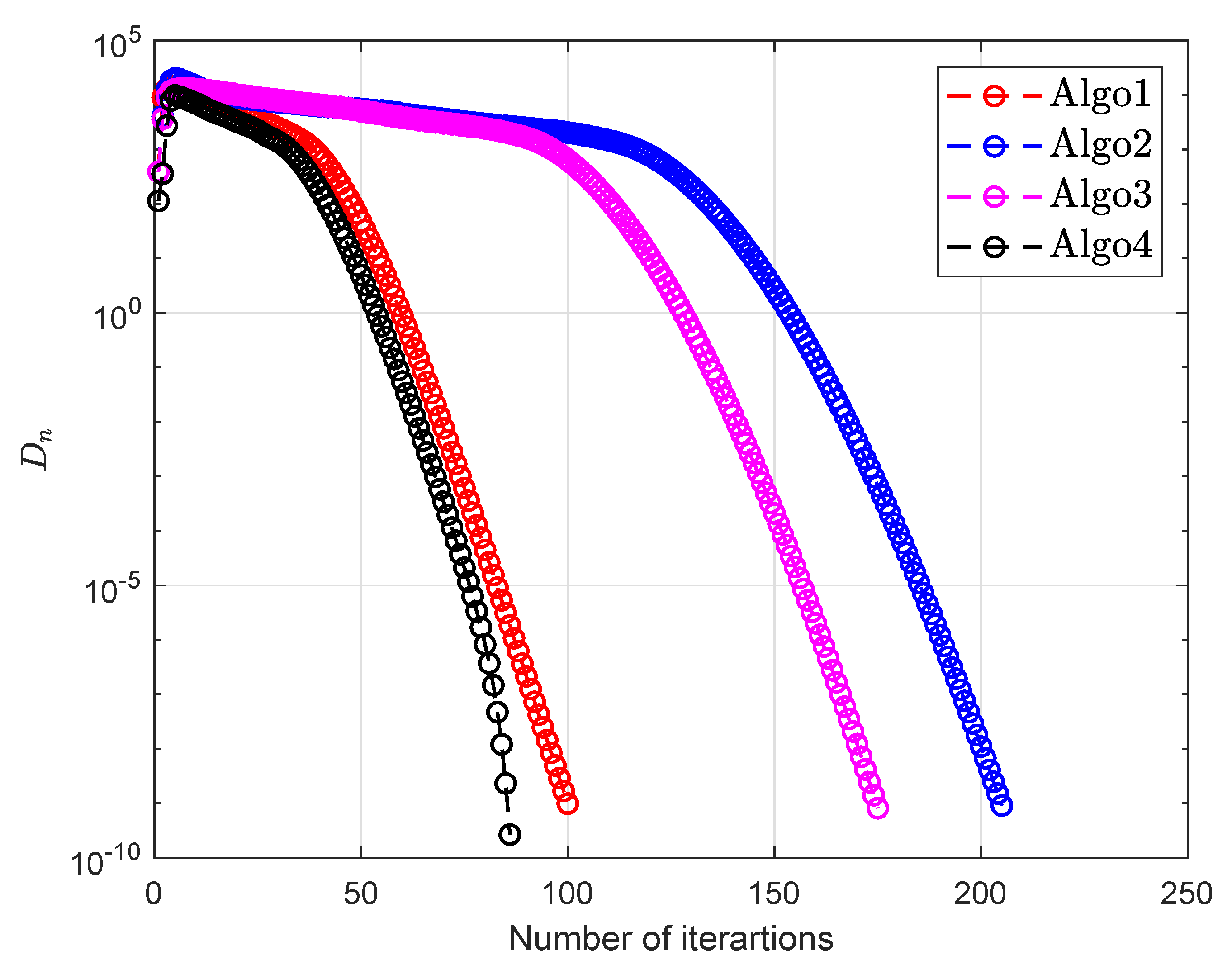
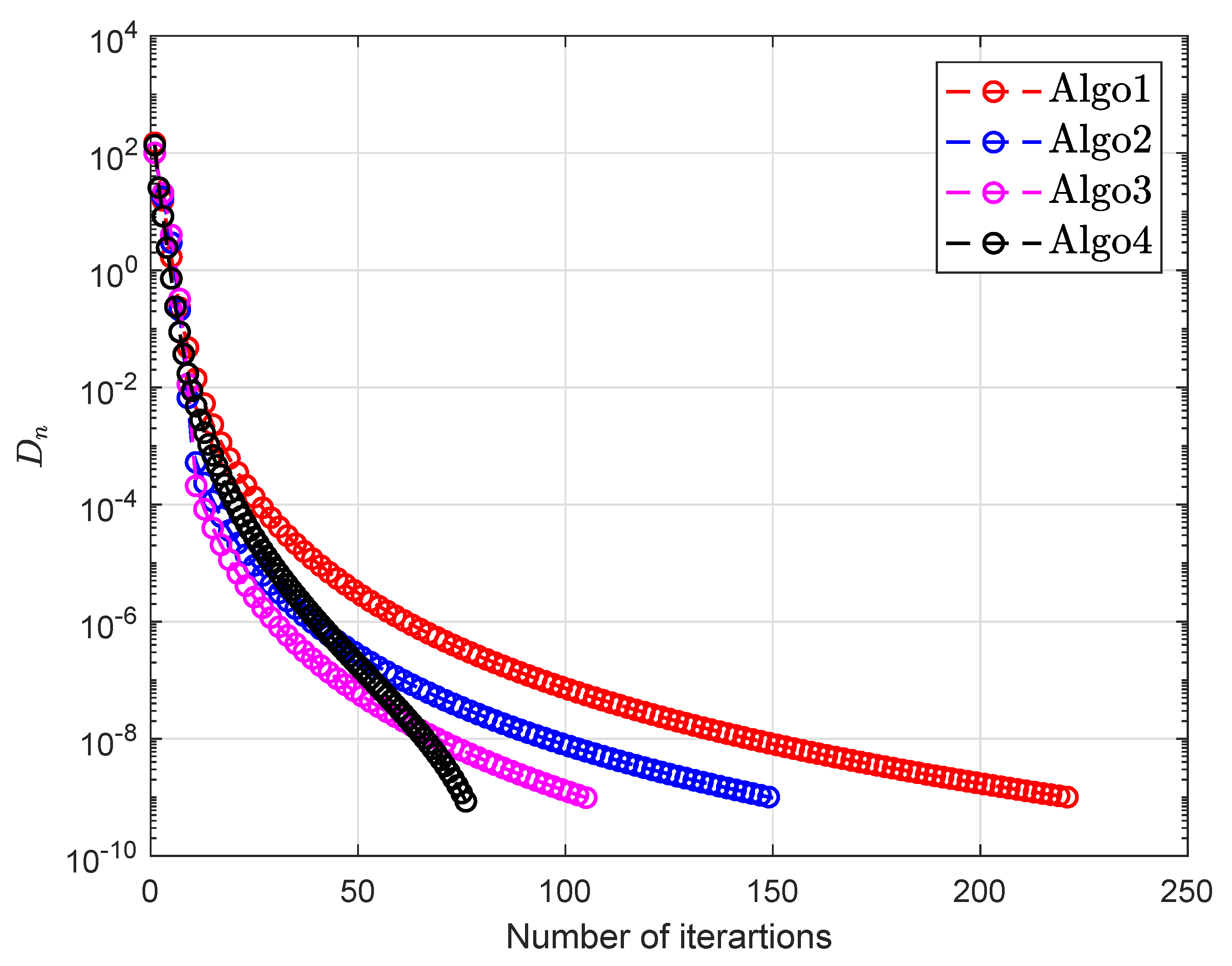
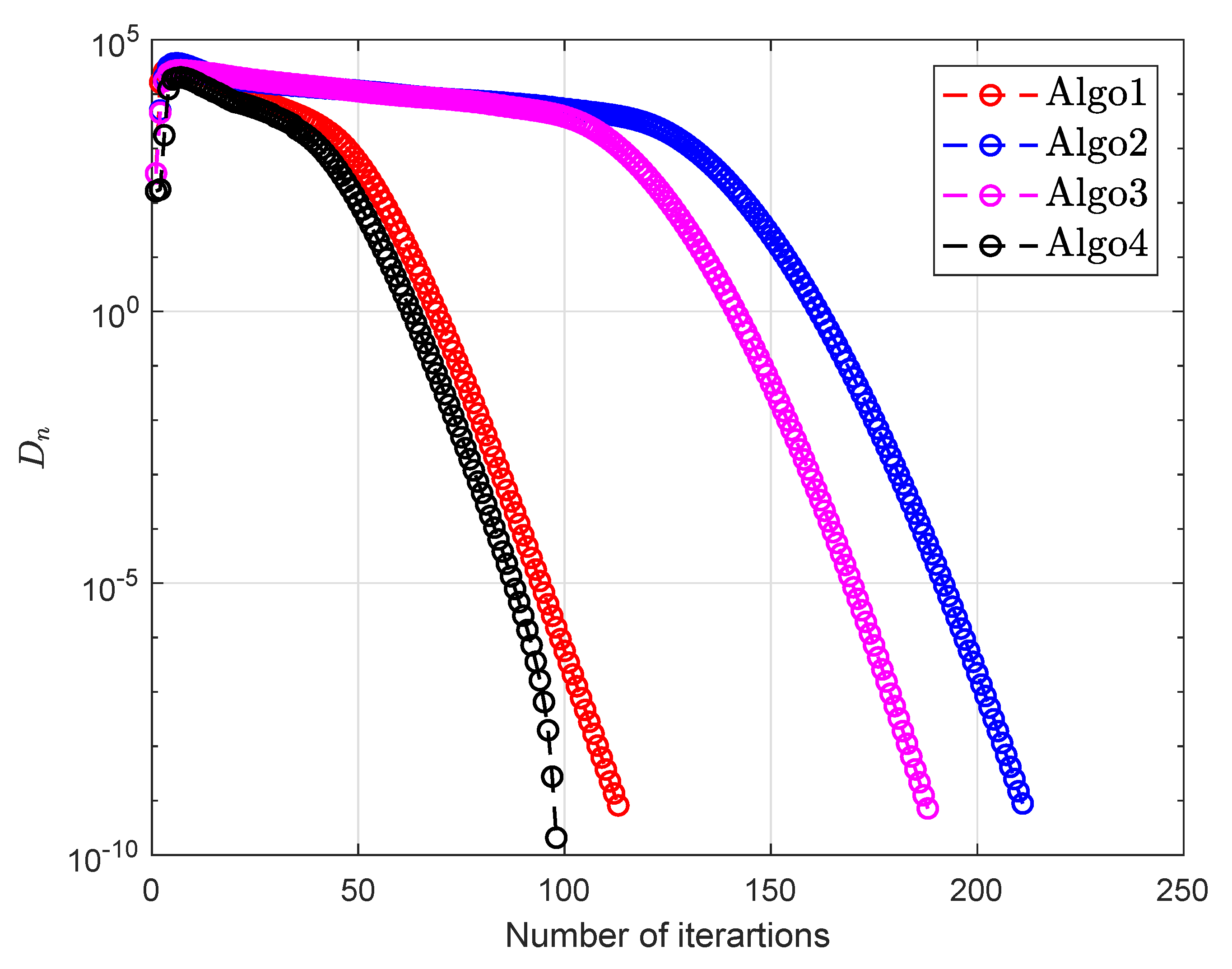
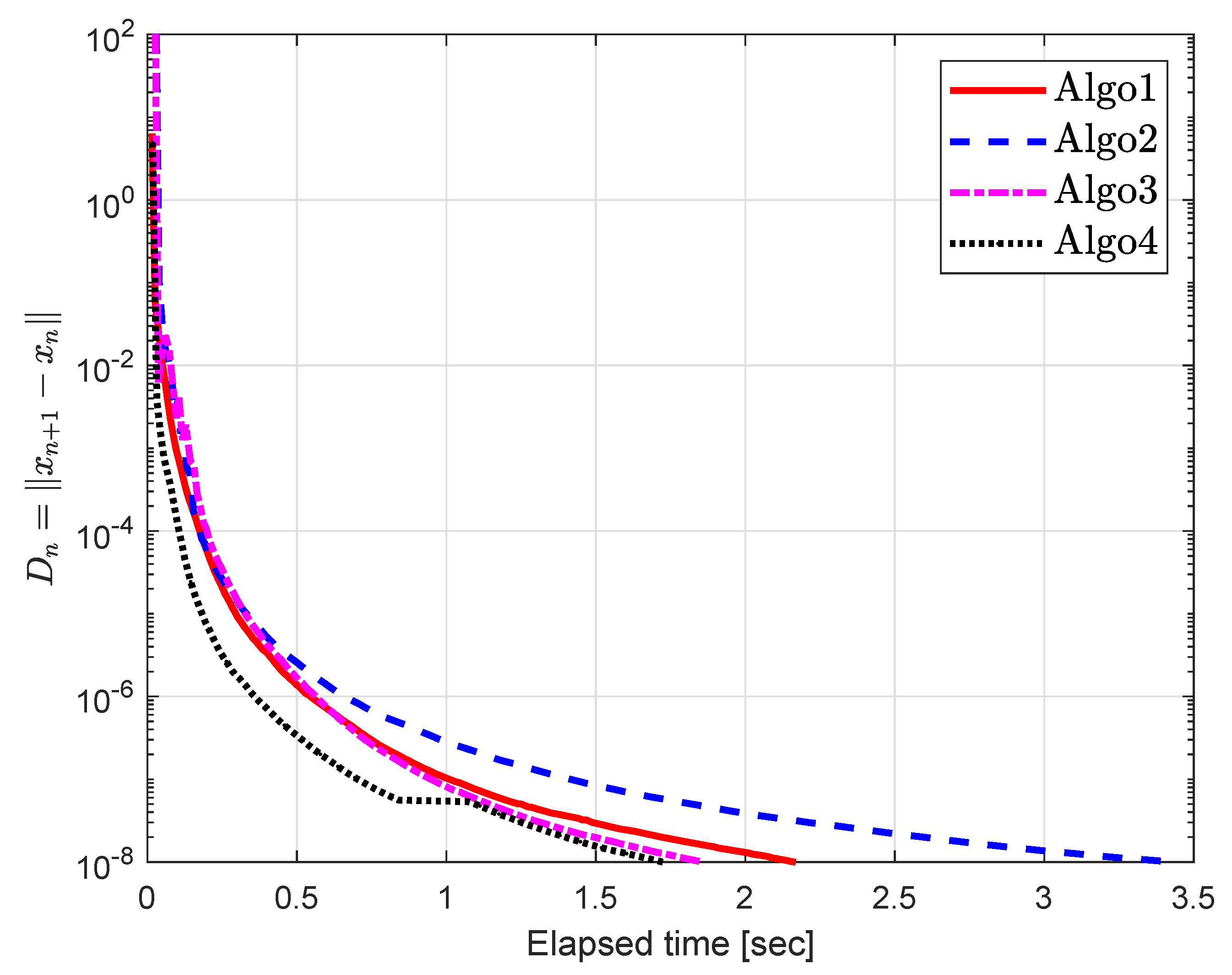
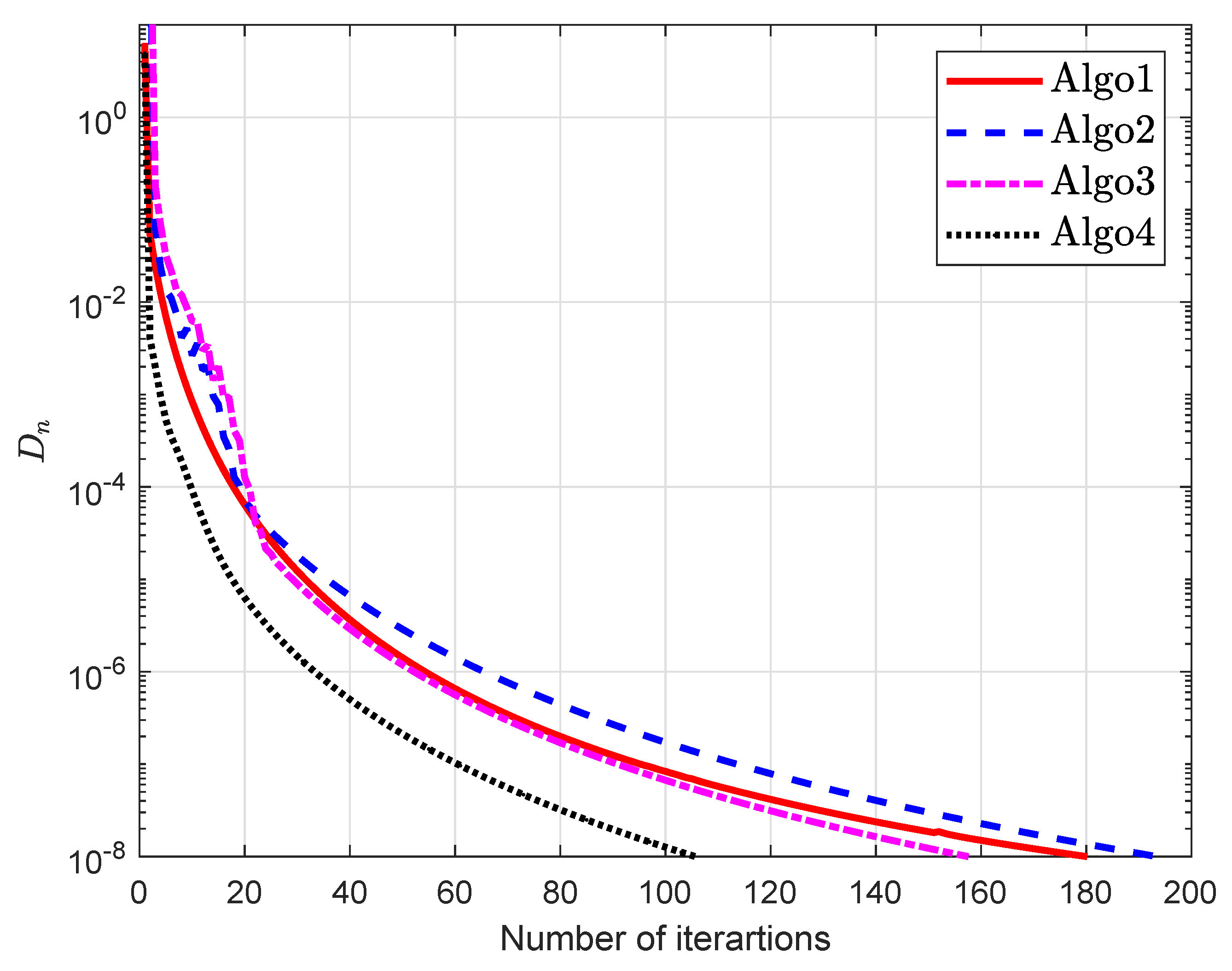
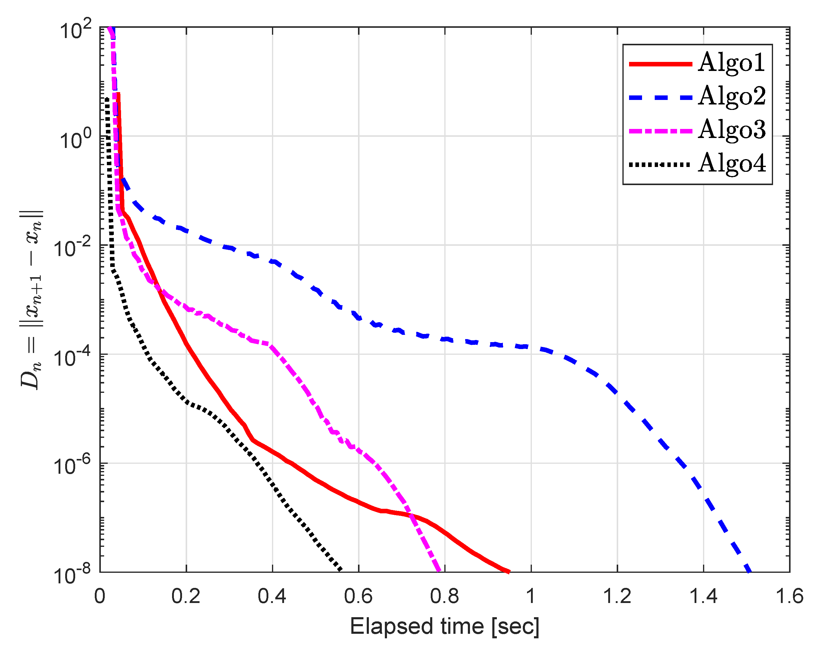
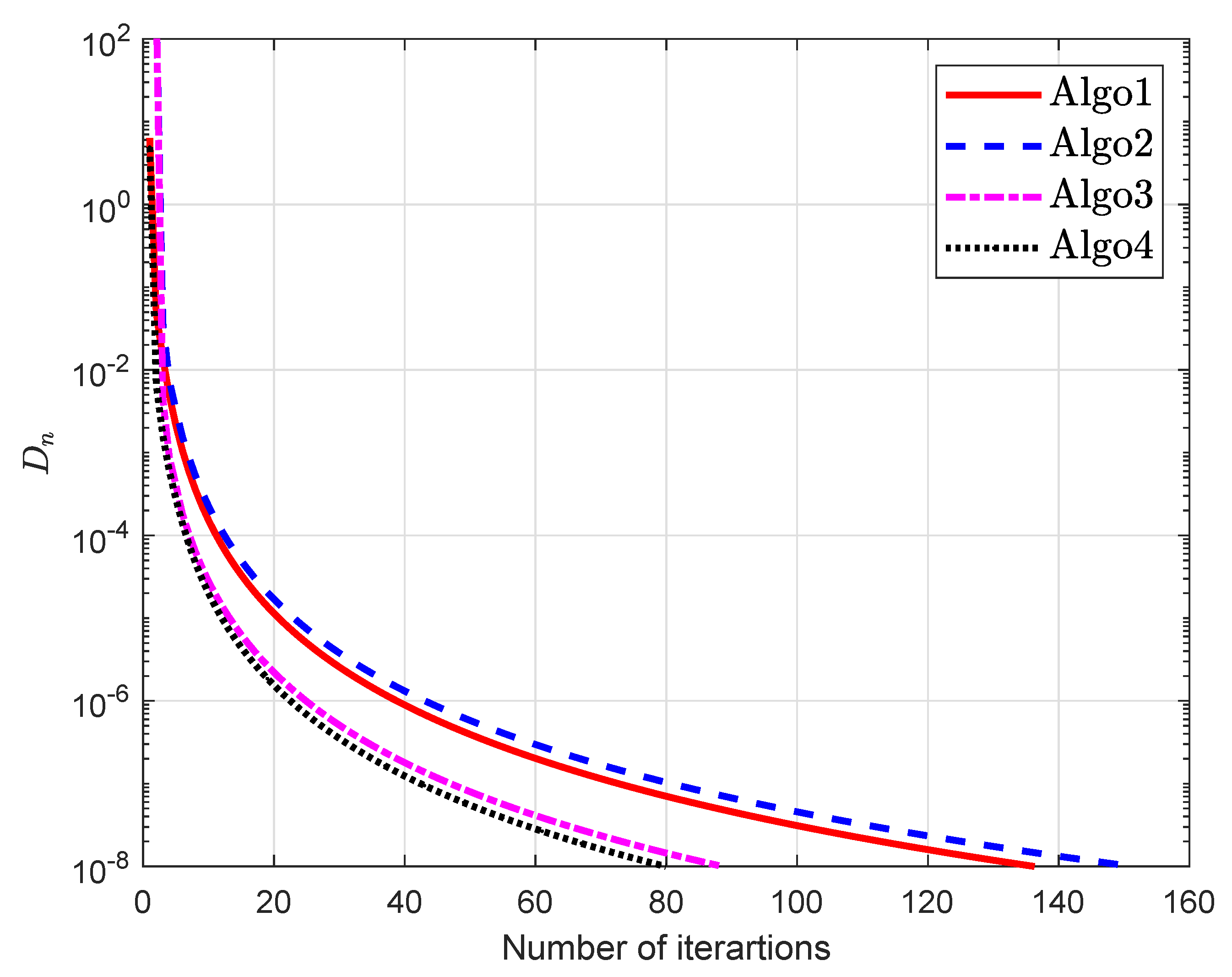
5. Computational Experiment
5.1. Example 1
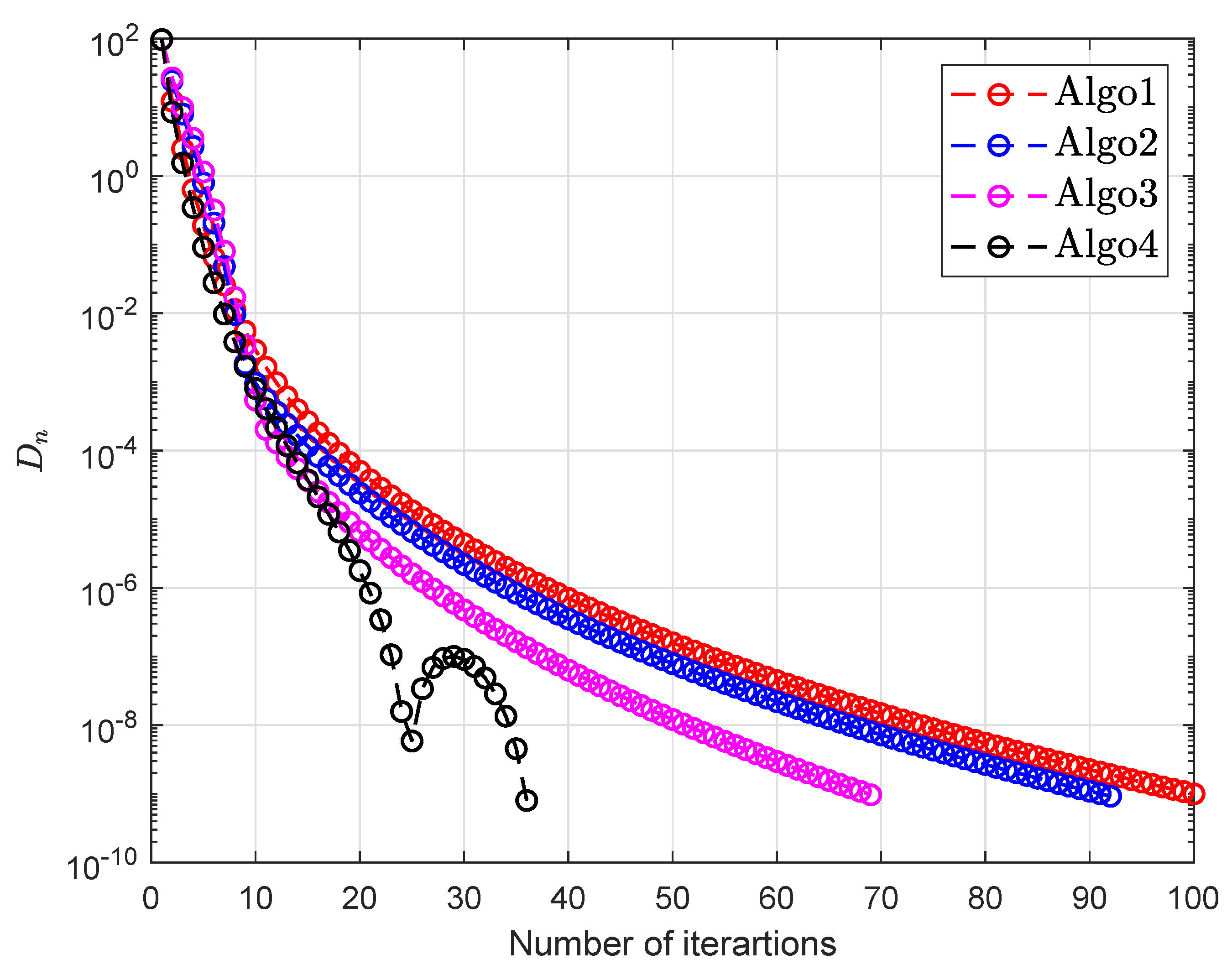
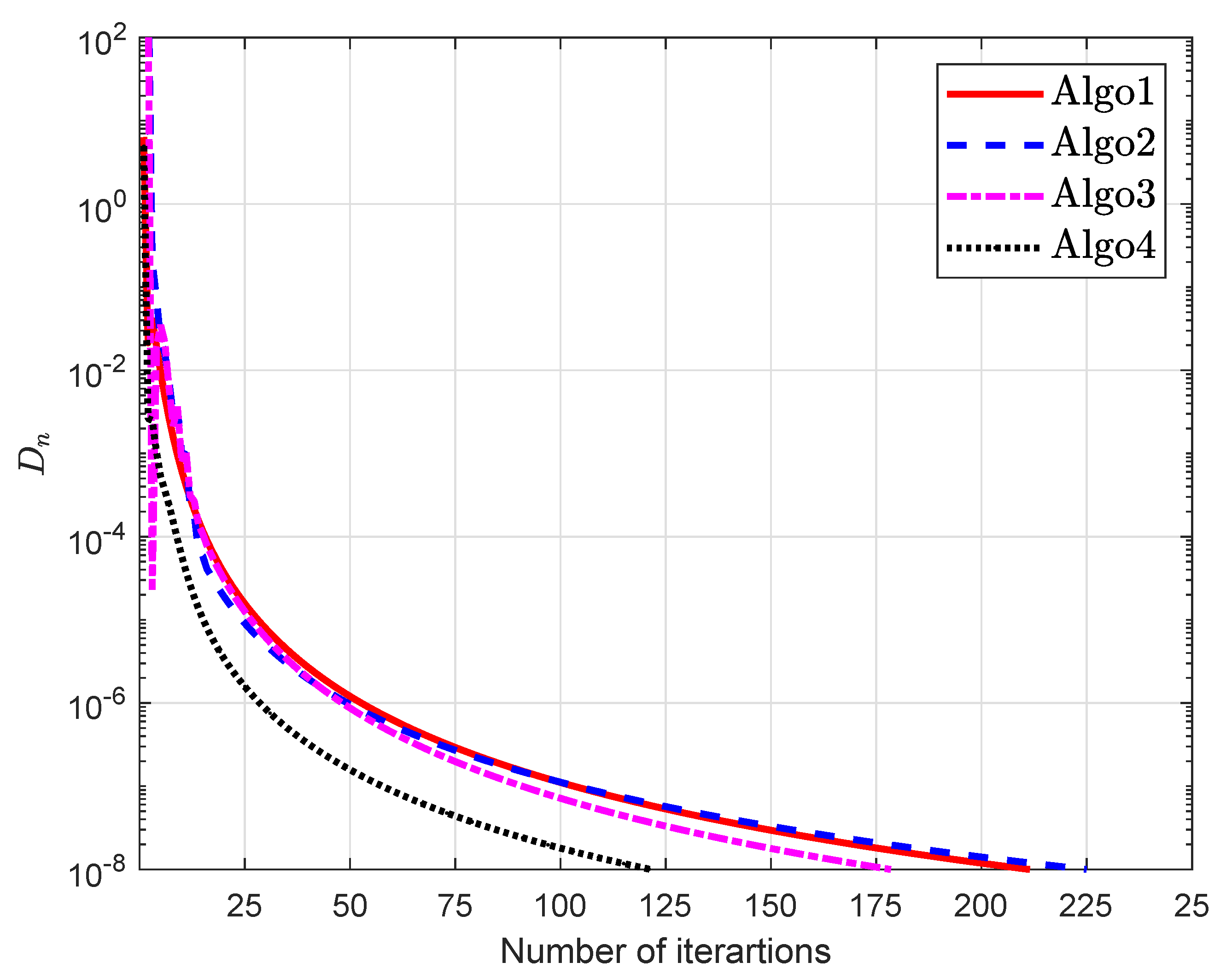
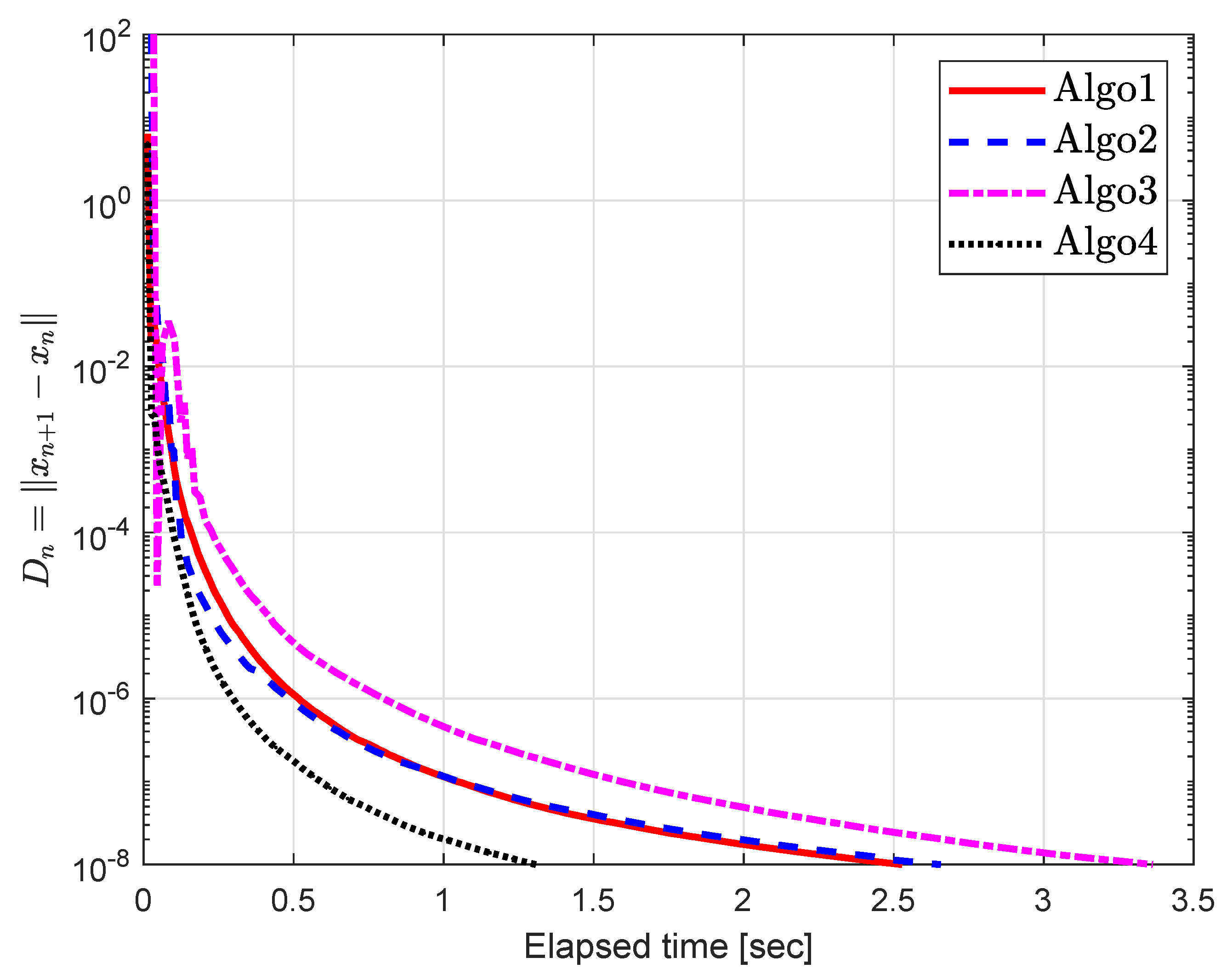
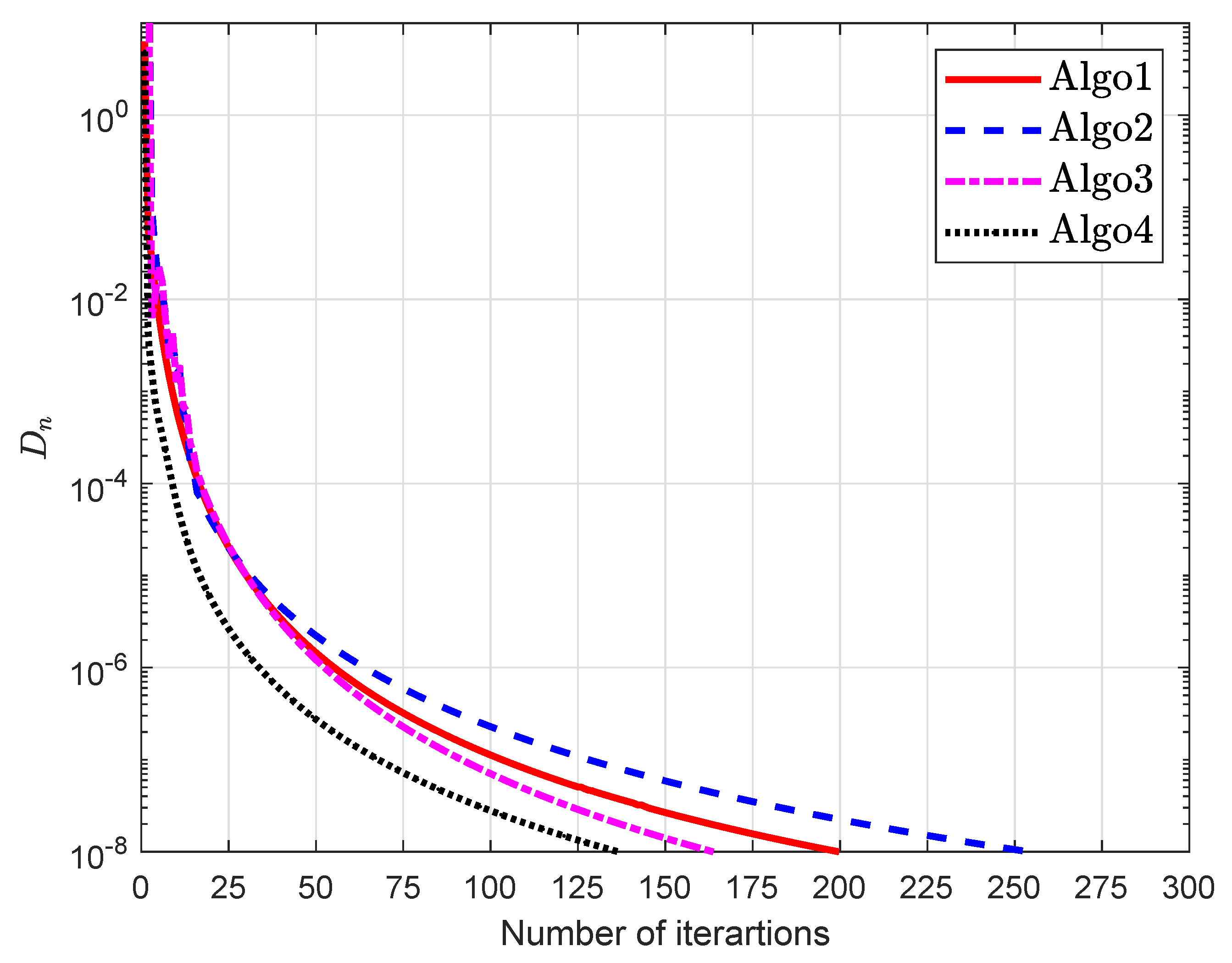
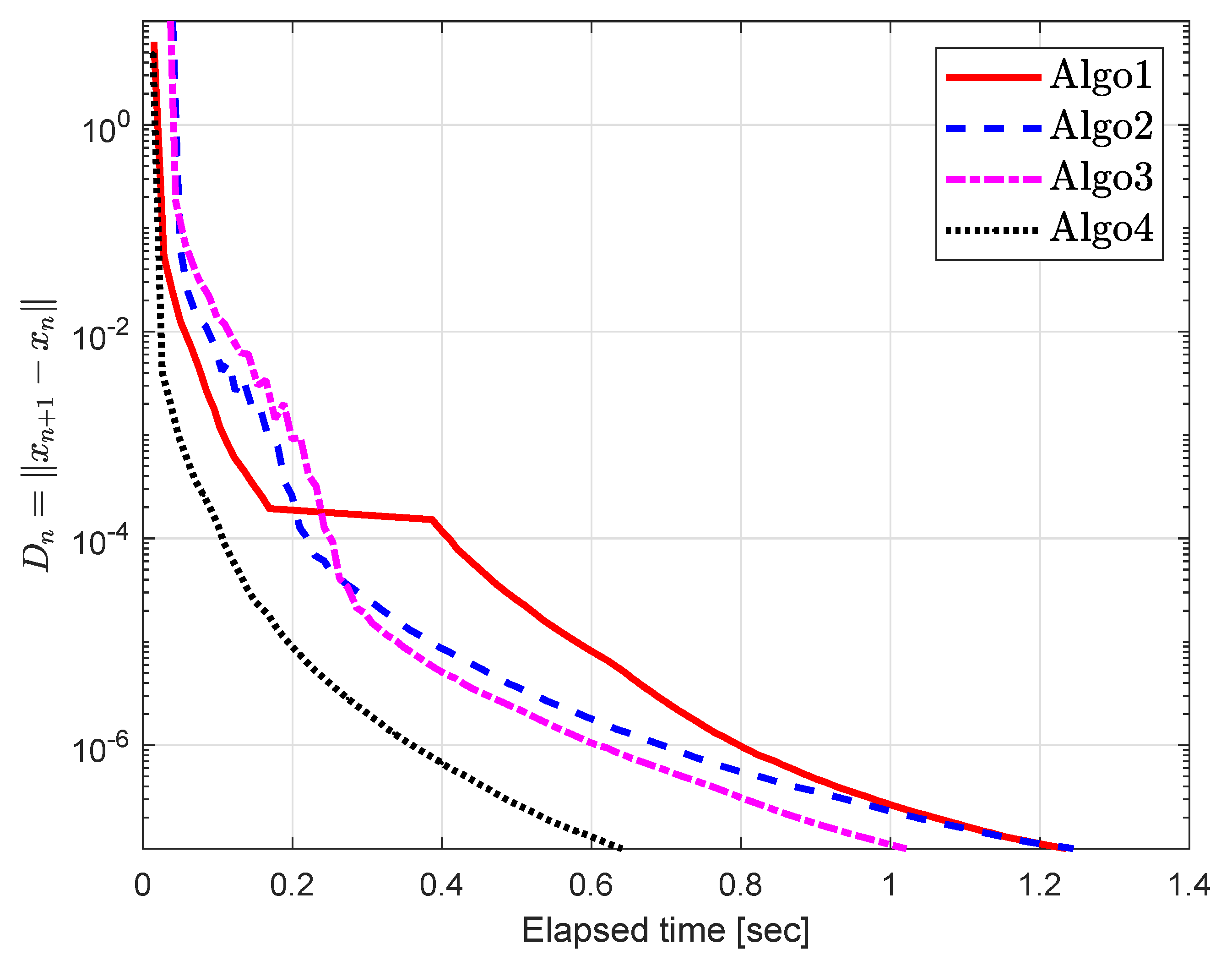
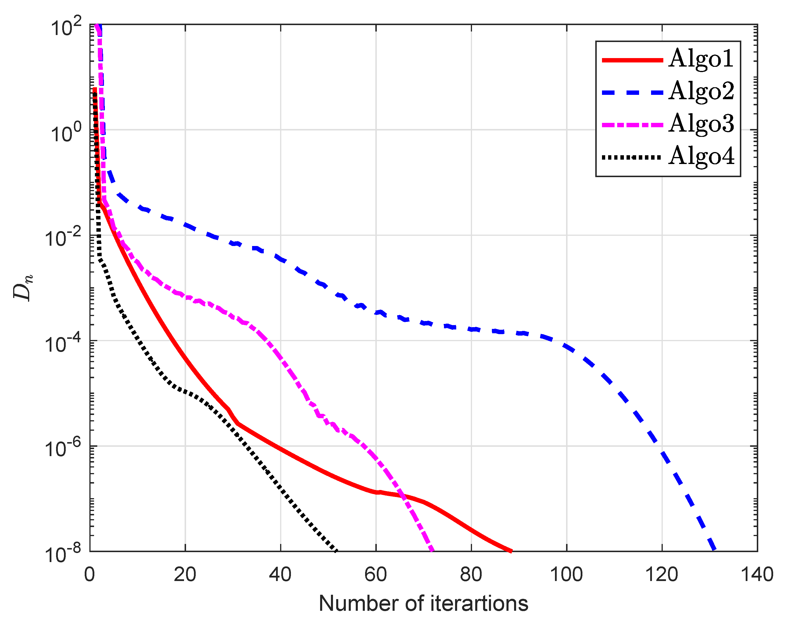
5.2. Example 2
- 1.
- There is no need to have prior knowledge of Lipschitz-constant for running algorithms on Matlab.
- 2.
- The convergence rate of the iterative sequence is based on the convergence rate of the stepsize sequence.
- 3.
- The convergence rate of the iterative sequence also depends on the nature of the problem and the size of the problem.
- 4.
- Due to the variable stepsize sequence, a particular value of the stepsize that is not suited to the current iteration of the algorithm often causes disturbance and hump in the behaviour of an iterative sequence.
6. Conclusions
Author Contributions
Funding
Acknowledgments
Conflicts of Interest
References
- Blum, E. From optimization and variational inequalities to equilibrium problems. Math. Stud. 1994, 63, 123–145. [Google Scholar]
- Dafermos, S. Traffic equilibrium and variational inequalities. Transp. Sci. 1980, 14, 42–54. [Google Scholar] [CrossRef] [Green Version]
- Ferris, M.C.; Pang, J.S. Engineering and economic applications of complementarity problems. Siam Rev. 1997, 39, 669–713. [Google Scholar] [CrossRef] [Green Version]
- Patriksson, M. The Traffic Assignment Problem: Models and Methods; Courier Dover Publications: Mineola, NY, USA, 2015. [Google Scholar]
- Facchinei, F.; Pang, J.S. Finite-Dimensional Variational Inequalities and Complementarity Problems; Springer Science & Business Media: Berlin, Germany, 2007. [Google Scholar]
- Konnov, I. Equilibrium Models and Variational Inequalities; Elsevier: Amsterdam, The Netherlands, 2007; Volume 210. [Google Scholar]
- Giannessi, F.; Maugeri, A.; Pardalos, P.M. Equilibrium Problems: Nonsmooth Optimization and Variational Inequality Models; Springer Science & Business Media: Berlin, Germany, 2006; Volume 58. [Google Scholar]
- Moudafi, A. Proximal point algorithm extended to equilibrium problems. J. Nat. Geom. 1999, 15, 91–100. [Google Scholar]
- Mastroeni, G. On auxiliary principle for equilibrium problems. In Equilibrium Problems and Variational Models; Springer: Berlin, Germany, 2003; pp. 289–298. [Google Scholar]
- Martinet, B. Brève communication. Régularisation d’inéquations variationnelles par approximations successives. ESAIM: Mathematical Modelling and Numerical Analysis—Modélisation Mathématique et Analyse Numérique 1970, 4, 154–158. [Google Scholar] [CrossRef] [Green Version]
- Rockafellar, R.T. Monotone operators and the proximal point algorithm. SIAM J. Control Optim. 1976, 14, 877–898. [Google Scholar] [CrossRef] [Green Version]
- Konnov, I. Application of the proximal point method to nonmonotone equilibrium problems. J. Optim. Theory Appl. 2003, 119, 317–333. [Google Scholar] [CrossRef]
- Antipin, A.S. The convergence of proximal methods to fixed points of extremal mappings and estimates of their rate of convergence. Comput. Math. Math. Phys. 1995, 35, 539–552. [Google Scholar]
- Combettes, P.L.; Hirstoaga, S.A. Equilibrium programming in Hilbert spaces. J. Nonlinear Convex Anal. 2005, 6, 117–136. [Google Scholar]
- Flåm, S.D.; Antipin, A.S. Equilibrium programming using proximal-like algorithms. Math. Prog. 1996, 78, 29–41. [Google Scholar] [CrossRef]
- Van Hieu, D.; Anh, P.K.; Muu, L.D. Modified hybrid projection methods for finding common solutions to variational inequality problems. Comput. Optim. Appl. 2017, 66, 75–96. [Google Scholar] [CrossRef]
- Van Hieu, D. Halpern subgradient extragradient method extended to equilibrium problems. Revista de la Real Academia de Ciencias Exactas, Fisicas y Naturales—Serie A: Matematicas 2017, 111, 823–840. [Google Scholar] [CrossRef]
- Argyros, I.K.; d Hilout, S. Computational Methods in Nonlinear Analysis: Efficient Algorithms, Fixed Point Theory and Applications; World Scientific: Singapore, 2013. [Google Scholar]
- Hieua, D.V. Parallel extragradient-proximal methods for split equilibrium problems. Math. Model. Anal. 2016, 21, 478–501. [Google Scholar] [CrossRef]
- Iusem, A.N.; Sosa, W. Iterative algorithms for equilibrium problems. Optimization 2003, 52, 301–316. [Google Scholar] [CrossRef]
- Quoc, T.D.; Anh, P.N.; Muu, L.D. Dual extragradient algorithms extended to equilibrium problems. J. Glob. Optim. 2012, 52, 139–159. [Google Scholar] [CrossRef]
- Quoc Tran, D.; Le Dung, M.; Nguyen, V.H. Extragradient algorithms extended to equilibrium problems. Optimization 2008, 57, 749–776. [Google Scholar] [CrossRef]
- Santos, P.; Scheimberg, S. An inexact subgradient algorithm for equilibrium problems. Comput. Appl. Math. 2011, 30, 91–107. [Google Scholar]
- Takahashi, S.; Takahashi, W. Viscosity approximation methods for equilibrium problems and fixed point problems in Hilbert spaces. J. Math. Anal. Appl. 2007, 331, 506–515. [Google Scholar] [CrossRef] [Green Version]
- Ur Rehman, H.; Kumam, P.; Cho, Y.J.; Yordsorn, P. Weak convergence of explicit extragradient algorithms for solving equilibirum problems. J. Inequalities Appl. 2019, 2019, 1–25. [Google Scholar] [CrossRef]
- Argyros, I.K.; Cho, Y.J.; Hilout, S. Numerical Methods for Equations and Its Applications; CRC Press: Boca Raton, FL, USA, 2012. [Google Scholar]
- Rehman, H.U.; Kumam, P.; Abubakar, A.B.; Cho, Y.J. The extragradient algorithm with inertial effects extended to equilibrium problems. Comput. Appl. Math. 2020, 39, 100. [Google Scholar]
- Rehman, H.U.; Kumam, P.; Cho, Y.J.; Suleiman, Y.I.; Kumam, W. Modified Popov’s explicit iterative algorithms for solving pseudomonotone equilibrium problems. Optim. Methods. Softw. 2020, 1–32. [Google Scholar] [CrossRef]
- Rehman, H.U.; Kumam, P.; Kumam, W.; Shutaywi, M.; Jirakitpuwapat, W. The Inertial Sub-Gradient Extra-Gradient Method for a Class of Pseudo-Monotone Equilibrium Problems. Symmetry 2020, 12, 463. [Google Scholar] [CrossRef] [Green Version]
- Hieu, D.V. New extragradient method for a class of equilibrium problems in Hilbert spaces. Appl. Anal. 2017, 1–14. [Google Scholar] [CrossRef]
- Polyak, B.T. Some methods of speeding up the convergence of iteration methods. USSR Comput. Math. Math. Phys. 1964, 4, 1–17. [Google Scholar] [CrossRef]
- Beck, A.; Teboulle, M. A fast iterative shrinkage-thresholding algorithm for linear inverse problems. SIAM J. Imaging Sci. 2009, 2, 183–202. [Google Scholar] [CrossRef] [Green Version]
- Dong, Q.L.; Lu, Y.Y.; Yang, J. The extragradient algorithm with inertial effects for solving the variational inequality. Optimization 2016, 65, 2217–2226. [Google Scholar] [CrossRef]
- Thong, D.V.; Van Hieu, D. Modified subgradient extragradient method for variational inequality problems. Numer. Algorithms 2018, 79, 597–610. [Google Scholar] [CrossRef]
- Dong, Q.; Cho, Y.; Zhong, L.; Rassias, T.M. Inertial projection and contraction algorithms for variational inequalities. J. Glob. Optim. 2018, 70, 687–704. [Google Scholar] [CrossRef]
- Yang, J. Self-adaptive inertial subgradient extragradient algorithm for solving pseudomonotone variational inequalities. Appl. Anal. 2019, 1–12. [Google Scholar] [CrossRef]
- Thong, D.V.; Van Hieu, D.; Rassias, T.M. Self adaptive inertial subgradient extragradient algorithms for solving pseudomonotone variational inequality problems. Optim. Lett. 2020, 14, 115–144. [Google Scholar] [CrossRef]
- Vinh, N.T.; Muu, L.D. Inertial Extragradient Algorithms for Solving Equilibrium Problems. Acta Math. Vietnam. 2019, 44, 639–663. [Google Scholar] [CrossRef]
- Van Hieu, D. Convergence analysis of a new algorithm for strongly pseudomontone equilibrium problems. Numer. Algorithms 2018, 77, 983–1001. [Google Scholar] [CrossRef]
- Hieu, D.V.; Cho, Y.J.; bin Xiao, Y. Modified extragradient algorithms for solving equilibrium problems. Optimization 2018, 67, 2003–2029. [Google Scholar] [CrossRef]
- Goebel, K.; Reich, S. Uniform Convexity. Hyperbolic Geometry, and Nonexpansive; CRC Press: Boca Raton, FL, USA, 1984. [Google Scholar]
- Bianchi, M.; Schaible, S. Generalized monotone bifunctions and equilibrium problems. J. Optim. Theory Appl. 1996, 90, 31–43. [Google Scholar] [CrossRef]
- Tiel, J.V. Convex Analysis; John Wiley: Hoboken, NJ, USA, 1984. [Google Scholar]
- Bauschke, H.H.; Combettes, P.L. Convex Analysis and Monotone Operator Theory in Hilbert Spaces; Springer: Berlin, Germany, 2011; Volume 408. [Google Scholar]
- Tan, K.K.; Xu, H.K. Approximating fixed points of non-expansive mappings by the Ishikawa iteration process. J. Math. Anal. Appl. 1993, 178, 301. [Google Scholar] [CrossRef] [Green Version]
- Ofoedu, E. Strong convergence theorem for uniformly L-Lipschitzian asymptotically pseudocontractive mapping in real Banach space. J. Math. Anal. Appl. 2006, 321, 722–728. [Google Scholar] [CrossRef] [Green Version]


| Algo1 [30] | Algo2 [39] | Algo3 [40] | Algo4 | |||||||
|---|---|---|---|---|---|---|---|---|---|---|
| n | N | iter. | time | iter. | time | iter. | time | iter. | time | |
| 10 | 10 | 83 | 0.8633 | 56 | 0.4295 | 35 | 0.2929 | 19 | 0.1319 | |
| 10 | 10 | 52 | 0.4297 | 64 | 0.4862 | 40 | 0.3040 | 23 | 0.1896 | |
| 10 | 10 | 94 | 0.8761 | 400 | 5.0501 | 305 | 3.4549 | 82 | 0.6732 | |
| 50 | 10 | 136 | 1.2545 | 107 | 0.9765 | 69 | 0.7521 | 54 | 0.4691 | |
| 50 | 10 | 86 | 0.6913 | 80 | 0.7453 | 55 | 0.4792 | 38 | 0.3128 | |
| 50 | 10 | 100 | 0.8427 | 205 | 2.2437 | 175 | 1.7925 | 86 | 0.7685 | |
| 100 | 10 | 222 | 3.0913 | 150 | 1.8105 | 105 | 1.1990 | 76 | 0.8656 | |
| 100 | 10 | 100 | 1.1624 | 92 | 1.0639 | 69 | 0.7964 | 36 | 0.4207 | |
| 100 | 10 | 113 | 1.3110 | 211 | 2.7524 | 188 | 2.4022 | 98 | 1.1311 | |
| Algo1 [30] | Algo2 [39] | Algo3 [40] | Algo4 | |||||||
|---|---|---|---|---|---|---|---|---|---|---|
| n | N | iter. | time | iter. | time | iter. | time | iter. | time | |
| 5 | 10 | 212 | 2.5360 | 225 | 2.6580 | 179 | 3.3746 | 122 | 1.3161 | |
| 5 | 10 | 200 | 2.1717 | 254 | 3.4295 | 164 | 1.8637 | 137 | 1.7299 | |
| 5 | 10 | 181 | 2.6688 | 194 | 2.3646 | 158 | 1.8703 | 106 | 1.1469 | |
| 5 | 10 | 89 | 0.9550 | 132 | 1.5186 | 72 | 0.7889 | 52 | 0.5644 | |
| 5 | 10 | 137 | 1.5127 | 152 | 1.8906 | 89 | 0.9427 | 80 | 0.8514 | |
© 2020 by the authors. Licensee MDPI, Basel, Switzerland. This article is an open access article distributed under the terms and conditions of the Creative Commons Attribution (CC BY) license (http://creativecommons.org/licenses/by/4.0/).
Share and Cite
Rehman, H.u.; Kumam, P.; Argyros, I.K.; Deebani, W.; Kumam, W. Inertial Extra-Gradient Method for Solving a Family of Strongly Pseudomonotone Equilibrium Problems in Real Hilbert Spaces with Application in Variational Inequality Problem. Symmetry 2020, 12, 503. https://0-doi-org.brum.beds.ac.uk/10.3390/sym12040503
Rehman Hu, Kumam P, Argyros IK, Deebani W, Kumam W. Inertial Extra-Gradient Method for Solving a Family of Strongly Pseudomonotone Equilibrium Problems in Real Hilbert Spaces with Application in Variational Inequality Problem. Symmetry. 2020; 12(4):503. https://0-doi-org.brum.beds.ac.uk/10.3390/sym12040503
Chicago/Turabian StyleRehman, Habib ur, Poom Kumam, Ioannis K. Argyros, Wejdan Deebani, and Wiyada Kumam. 2020. "Inertial Extra-Gradient Method for Solving a Family of Strongly Pseudomonotone Equilibrium Problems in Real Hilbert Spaces with Application in Variational Inequality Problem" Symmetry 12, no. 4: 503. https://0-doi-org.brum.beds.ac.uk/10.3390/sym12040503