On the Dynamics of a Visco–Piezo–Flexoelectric Nanobeam

Abstract

The fundamental motivation of this research is to investigate the effect of flexoelectricity on a piezoelectric nanobeam for the first time involving internal viscoelasticity. To date, the effect of flexoelectricity on the mechanical behavior of nanobeams has been investigated extensively under various physical and environmental conditions. However, this effect as an internal property of materials has not been studied when the nanobeams include an internal damping feature. To this end, a closed-circuit condition is considered taking converse piezo–flexoelectric behavior. The kinematic displacement of the classical beam using Lagrangian strains, also applying Hamilton’s principle, creates the needed frequency equation. The natural frequencies are measured in nanoscale by the available nonlocal strain gradient elasticity model. The linear Kelvin–Voigt viscoelastic model here defines the inner viscoelastic coupling. An analytical solution technique determines the values of the numerical frequencies. The best findings show that the viscoelastic coupling can directly affect the flexoelectricity property of the material.

1. Introduction

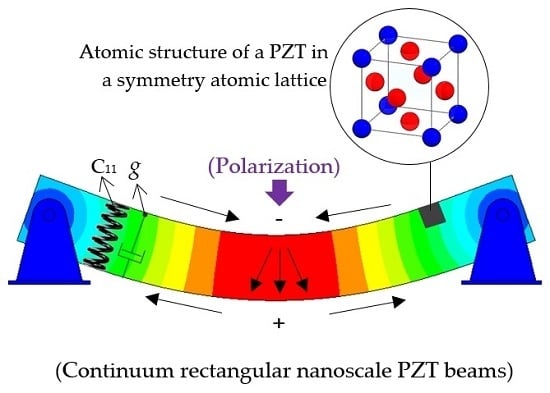
Flexoelectricity can be described as a general electromechanical linear coupling effect between the electric polarization and the strain gradient and, conversely, the electric field gradient and the elastic strain. This phenomenon can be considered as a higher-order effect than piezoelectricity, which is the polarization response to the strain. The flexoelectric effect can be understood from the piezoelectric effect. In piezoelectric material, when the material is bent, compressed, or tensioned, it gives the electric field itself, and vice versa. In flexoelectric material, also by mechanical deformation of the material, the electric field can be obtained, and vice versa. This effect can be applied to next-generation sensors, actuators, and MEMS/NEMS (micro-/nanoelectromechanical systems). Nonetheless, at the nanoscale where large strain gradients are expected, the flexoelectric effect is significant. The gradient effect shows that the importance of the flexoelectric effect on micro- and nanosystems is comparable to that of piezoelectricity and even beyond it. In addition, unlike piezoelectricity, flexoelectricity is found in any material with any symmetry. This means that unlike piezoelectricity, which is invalid and inefficient in materials with central symmetry, there are effects of flexoelectricity in all biological materials and systems. In fact, the superiority of this effect over the piezoelectric effect is that piezoelectricity can occur in only 20 types of crystal structures, but the flexoelectric effect is not limited. These features have led to a growing interest in flexoelectricity in the last decade [1,2,3].

Currently, studies on the role of flexoelectricity in dielectric physics have been performed and have shown promising practical applications. On the other hand, the discrepancy between theoretical and empirical results indicates limited understanding in this area. A homogeneous deformation or a strain gradient induces flexoelectricity; on the other side, an inhomogeneous deformation induces piezoelectricity. Accordingly, the effects of flexoelectricity on nanoscale systems are significantly higher than those on macroscale systems in light of the fact that the strain gradient fits inversely to the element size [1,2,3,4,5,6,7,8].

Lately, in both theoretical and experimental studies, a surge of scientific interest has been stimulated concerning flexoelectricity, particularly for small-scale piezoelectric materials. Estimation of the physics of piezo–flexoelectric coupling factors has been performed with success in some experiments [4,5,6,7,8,9,10,11,12,13].

In addition to studying the physics of piezoelectric–flexoelectric nanomaterials, another aspect of assessing piezoelectric–flexoelectric effects in nanostructures is the prediction of the mechanical behavior of a nanoscale material while it contains piezoelectricity or flexoelectricity or even both effects simultaneously. Piezoelectric effects alone have been estimated based on the mechanical behavior of nanostructures in the current decade [14,15,16,17,18,19,20,21,22,23]. However, the combination of the flexoelectricity effect and piezoelectricity influence is a new physical composition. In the literature on the mechanical behavior of nanostructures, the influences of flexoelectric phenomena have been investigated based on the mechanical response of piezoelectric nanobeam structures. In terms of the static deflections and bending problems of a nanobeam, Liang et al. [24] developed a piezoelectric cantilever nanobeam based on the flexoelectricity and surface effects. The proposed beam model used Euler–Bernoulli to implement electromechanical coupling in a bending analysis for which the piezoelectricity, dielectricity, and surface elasticity, particularly flexoelectricity, were considered. Zhang et al. [25] modeled a higher-order beam as a dielectric piezoelectric beam and studied the influences of flexoelectricity, while the static deflections were given for hinged–hinged and cantilever beams. Qi et al. [26] investigated a double-layered piezoelectric nanobeam regarding flexoelectric coupling under static bending conditions. The achieved equations were established based on the Euler–Bernoulli beam and solved on the basis of open- and closed-circuit cases. Sneha Rupa and Ray [27], based on the nonlocality of Eringen, analyzed the flexoelectricity behavior of pivot–pivot piezoelectric nanobeams. They worked on both direct and indirect flexoelectric influences and extracted the numerical outcomes of linear static bending with regard to an exact solution. Xiang and Li [28] derived an exact elasticity solution to analyze the bending of a nanosize beam, including piezoelectricity and flexoelectricity, by using strain gradient elasticity. Zarepour et al. [29] studied nonlinearity based on the geometrical phenomenon in order to consider flexoelectricity in a nanosize piezoelectric beam. The beam hypothesis was Timoshenko, and the treatment of a small scale was shown by the nonlocal elasticity theory. The formulated theoretical relations were solved by utilizing the Galerkin method for fixed–fixed and pivot–pivot edge conditions. Yang et al. [30] employed the finite element method to develop flexoelectricity effects for a piezoelectric nanobeam. According to the strain gradient elasticity model, based on the linear Lagrangian strains and by means of the classic beam approach, the static deflections of the cantilever beam were determined. Zhao et al. [31] nonlinearly investigated the bending analysis of a nanoscale piezoelectric beam involving flexoelectricity impacts and incorporating surface influences on the basis of the strain gradient elasticity model. They adjusted the Timoshenko beam model to derive the required equilibrium equations and discretized the equations by means of the generalized differential quadrature (GDQ) method. Thereafter, an iteration method was applied to solve the discretized equations. Basutkar et al. [32] produced an analysis of the static bending of a piezoelectric nanobeam that possesses flexoelectricity influences and incorporated surface effects based on the element-free Galerkin method.

In the case of the bending of piezoelectric–flexoelectric nanostructures with plate-like shapes, Ghobadi et al. [33] evaluated the effect of nano size with the help of classical plate theory to study the static bending of a nanoplate exposed to thermal, electric, and magnetic fields, assuming piezoelectricity and flexoelectricity properties.

Moreover, in terms of static instability and buckling of piezoelectric–flexoelectric nanobeams, Ebrahimi and Karimiasl [34] calculated the stability capacity of a sandwich nanobeam system by taking the piezoelectricity–flexoelectricity effects into account on the basis of the stress nonlocality hypothesis and considering surface effects. The Navier method was applied to solve the equations which resulted from the Euler–Bernoulli kinematic model.

On the other hand, in the discussion of specific piezoelectric–flexoelectric nanostructures, e.g., nanoshells, Zeng et al. [35] analytically analyzed the static instability situation of a piezoelectric nanoshell while examining the flexoelectric property. Study of the small scale was captured via the couple stress model, and the kinematic displacement was estimated according to the shear deformable shell model.

Further, in the field of dynamic analyses of piezoelectric nanobeams under the flexoelectricity phenomenon, Barati [36] nonlinearly studied the frequencies of a piezoelectric nanobeam involving flexoelectric effects subjected to thermal surroundings. The surface effect was placed in the constitutive equations which originated from the classical beam approach, and He’s variational method was used to derive the equations. Generally, the natural frequencies of the problem were computed by the use of the Galerkin method. Arefi et al. [37] investigated the effects of residual stress, surface, small scale, and flexoelectricity on a Timoshenko piezoelectric nanobeam while considering functionality in different cases, i.e., simple, sigmoid, and exponential power indices. A cubically nonlinear foundation was modeled and placed. The differential quadrature (DQ) method discretized the equations of frequency, and a direct iterative process computed the values of the frequencies. Ebrahimi and Barati [38] analytically researched the vibration response of a piezoelectric nanobeam embedded on the Winkler–Pasternak foundation. They considered classical beam theory and took flexoelectricity and surface effects together in the frequency equations. The vibration relations were combined with nonlocal continuum theory. Furthermore, Amiri et al. [39], based on the Euler–Bernoulli beam and nonlocal strain gradient size-dependent model, simulated the instability and free vibrations of a piezoelectric nanotube, taking surface and flexoelectric influences into consideration in the evaluation. Parsa and Mahmoudpour [40] assumed an initial curvature for a piezoelectric nanobeam to study the effect of flexoelectricity on such a specimen. The classic beam model was used, and the nonlocal strain gradient was combined into the equations of motion to survey the small scale. A foundation which included the linear and nonlinear transverse effects and a shear coefficient was bridged for the system. Vaghefpour and Arvin [41] modeled a nanobeam as a cantilever beam and studied its natural frequencies with respect to the thin beam model by applying both piezoelectricity and flexoelectricity. Different solution procedures were employed, namely, the Galerkin projection and Lindstedt–Poincaré technique.

In addition to the above literature, Fattahian Dehkordi and Tadi Beni [42], by use of a consistent couple stress model, investigated analytically the natural frequencies of a nanocone based on the piezoelectric–flexoelectric coupling. The nanocone was modeled with single wall. The governing equations were attained on the basis of Love’s thin shell theory and linear Lagrangian strains.

Also, a special investigation can be found in [43], in which double cantilever piezoelectric nanobeams were analyzed, for which the flexoelectricity property was also taken into account. A crack was assumed in the beam, and the strain gradient elasticity theory was employed to capture the size dependency.

Another type of material property is internal viscoelasticity by which an unsteady outer excitation frequency can be damped [44,45,46]. Unlike the many kinds of research done on piezoelectric nanobeams by studying flexoelectric influence, there are no reports about piezoelectric–flexoelectric nanobeams considering inner viscoelasticity. However, in the category of the combination of piezoelectricity with internal viscoelasticity, there can be seen a few published papers. Li et al. [47] inspected the buckling and vibrations of axially moving nanoplates considering piezoelectricity and viscoelasticity coupling. They considered the thermal environment as well. Nonlocal framework was done using nonlocal elasticity theory. The attained values of the buckling and natural frequency on the basis of a Galerkin numerical solution technique. Zenkour and Sobhy [48] studied the nonlocal natural frequencies of a piezoelectric nanoplate assuming viscoelastic coupling based on the Kelvin–Voigt model and also embedding the plate on a viscoelastic matrix. The hygral and thermal effects of the environment were also investigated. The governing equations were gained on the basis of a two-variable refined higher-order shear deformation approach in combination with nonlocal elasticity. Tadi Beni et al. [49] analyzed the nonlinear resonance frequencies of a piezoelectric Euler–Bernoulli nanobeam by taking the viscoelasticity effect. The nanoscale size influence was considered on the basis of a coupled stress approach. The obtained nonlinear frequency relation was solved using the Galerkin method.

Since viscoelastic coupling may affect the role of flexoelectricity in a piezoelectric material, understanding this effect can be important. It should be kept in mind that viscoelastic coupling is not limited to considering this property in the material; it can also be investigated in the boundary conditions [50,51]. This research examines the current knowledge of flexoelectricity in piezoelectric nanobeams, whilst the Kelvin–Voigt viscoelastic model is investigated for the material. The closed-circuit condition is applied for a reverse flexoelectric status. The combined flexoelectric and viscoelastic terms are implemented in the Euler–Bernoulli beam estimated in the nanoscale using the nonlocal strain gradient model. The analytical solution procedure is demonstrated to numerically present the results. A validation section was prepared to illustrate the precision and accuracy of the present formulation. A conclusion section is also provided to give the significant findings in brief.

2. The Visco–Piezo–Flexoelectric Model

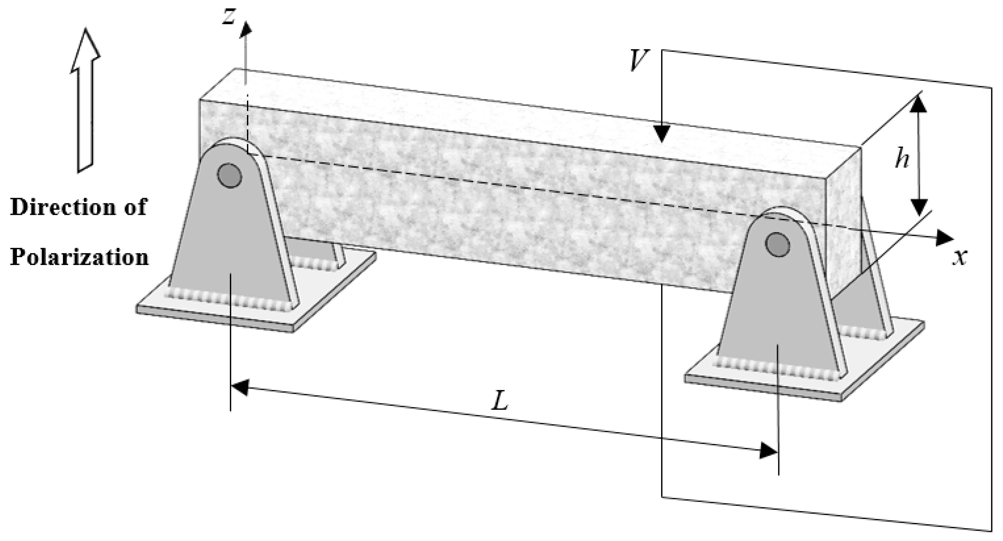
The visco–piezo–flexoelectric nanobeam analyzed in this research is illustrated in Figure 1. In the figure, the length and height of the beam are denoted L and h, respectively.

2.1. Piezo–Flexoelectricity

To introduce the flexoelectricity influence, it should be noted that the electric field gradient produces an elastic strain field (converse effect) and the elastic strain gradient induces electric polarization (direct effect). The density of total internal energy of a bulk piezo–flexoelectric material is [29,36]

$$\begin{array}{l}{\prod }_b=\frac{1}{2}{a}_{kl}{P}_k{P}_l+\frac{1}{2}{C}_{ijkl}{\epsilon }_{ij}{\epsilon }_{kl}+d_{ijk}{P}_k{\epsilon }_{ij}+\frac{1}{2}{b}_{ijkl}\frac{\partial P_i}{\partial x_j}\frac{\partial P_k}{\partial x_l}+f_{ijkl}\frac{\partial {\epsilon }_{ij}}{\partial x_l}{P}_k\\ -f_{ijkl}{\epsilon }_{ij}\frac{\partial P_k}{\partial x_l}\cdot \end{array}$$

(1)

The constitutive equations based on Equation (1) can be derived as

$${\sigma }_{ij}=\frac{\partial {\Pi }_b}{\partial {\epsilon }_{ij}}=C_{ijkl}{\epsilon }_{kl}+d_{ijk}{P}_k-f_{ijkl}\frac{\partial P_k}{\partial x_l}\cdot$$

(2)

$${\xi }_{ijl}=\frac{\partial {\Pi }_b}{\partial \left(\frac{\partial {\epsilon }_{ij}}{\partial x_l}\right)}=f_{ijkl}{P}_k\cdot$$

(3)

$$E_i=\frac{\partial {\Pi }_b}{\partial P_i}=a_{ij}{P}_j+d_{jki}{\epsilon }_{jk}+f_{klji}\frac{\partial {\epsilon }_{kl}}{\partial x_j}\cdot$$

(4)

$$q_{ij}=\frac{\partial {\Pi }_b}{\partial \left(\frac{\partial P_i}{\partial x_j}\right)}=b_{ijkl}\frac{\partial P_k}{\partial x_l}-f_{klij}{\epsilon }_{kl}\cdot$$

(5)

in which ${\epsilon }_{kl}$ are the elastic strains, $C_{ijkl}$ are the elastic coefficients, $E_k$ is the electric field, ${\sigma }_{ij}$ is the so-called equilibrium stress tensor, $f_{ijkl}$ denotes the fourth-order flexoelectric tensor related to the direct flexoelectric effect, $a_{ij}$ represents the reciprocal dielectric susceptibility (second-order dielectric tensor), $P_i$ is electric polarization, $d_{ijk}$ is the piezoelectric modulus, $b_{ijkl}$ is the coupling between polarization gradients, ${\xi }_{ijl}$ is the induction of the converse flexoelectric effect and called the higher-order moment stress tensor, and $q_{ij}$ is the electric quadrupole density due to flexoelectricity.

The chosen beam theory for this study is Euler–Bernoulli [52,53]:

$$u_1\left(x,z,t\right)=-z\frac{\partial w\left(x,t\right)}{\partial x},$$

(6)

$$u_3\left(x,z,t\right)=w\left(x,t\right)\cdot$$

(7)

where u_i (i = 1,3) represents the points’ displacements in the x and z directions, and w is the lateral displacement of the midplane. To show the thickness coordinate, the z parameter is used, and t is demonstrative of time.

As the problem considered in this research is linear vibration analysis, the linear Lagrangian strain can be presented as

$${\epsilon }_{ij}=\frac{1}{2}\left(u_{i,j}+u_{j,i}\right)\cdot$$

(8)

Applying Equation (8) to Equations (6) and (7) gives the elastic strains in the case of displacements as follows:

$${\epsilon }_{xx}=-z\frac{{\partial }^{2}w}{\partial x^2},$$

(9)

$${\eta }_{xxx}=\frac{\partial {\epsilon }_{xx}}{\partial x}=-z\frac{{\partial }^{3}w}{\partial x^3},$$

(10)

$${\eta }_{xxz}=\frac{\partial {\epsilon }_{xx}}{\partial z}=-\frac{{\partial }^{2}w}{\partial x^2}\cdot$$

(11)

As ${\eta }_{xxx}$ is small relative to ${\eta }_{xxz}$, it can be neglected. The transverse direction was chosen for the direction of polarization. Thus, the relationship between the electric field and electric potential based on the Maxwell electric field relation in the transverse direction is as follows:

$$E_z+\frac{\partial \Phi }{\partial z}=0$$

(12)

in which $\Phi$ denotes the electric potential. Inserting Equation (11) into Equation (4) yields the effective local electric field equation as below:

$$E_z=a_{33}{P}_z+d_{31}\left(-z\frac{{\partial }^{2}w}{\partial x^2}\right)-f_{31}\frac{{\partial }^{2}w}{\partial x^2}\cdot$$

(13)

Gauss’s law is expressed as follows, where the free electric body charges are ignored [29]:

$$-\kappa \frac{{\partial }^2\Phi }{\partial z^2}+\frac{\partial P_z}{\partial z}=0\cdot$$

(14)

Here, $\kappa ={\kappa }_1{\kappa }_2$ is the permittivity (electric polarizability measure for a dielectric material), ${\kappa }_1$ exhibits the background permittivity of the piezo–flexoelectric material, and ${\kappa }_2$ denotes the permittivity of the air. Physically, permittivity directly affects the polarization, which means that in response to an external electric field, a material with higher permittivity polarizes further.

In a converse effect and for a closed-circuit condition, the electric boundary conditions can be defined as

$$\Phi \left(\frac{h}{2},t\right)=V,\hspace{1em}\Phi \left(-\frac{h}{2},t\right)=0\cdot$$

(15)

in which V denotes the external electric voltage. Combining Equation (12), Equation (13), and Equation (15) into Equation (14), we present the electrical polarization, electric field component, and electric potential as [36]

$$P_z=-\frac{V}{a_{33}h}+\left(\frac{\kappa d_{31}z}{\left(1+a_{33}\kappa \right)}+\frac{f_{31}\left(1+2a_{33}\kappa \right)}{a_{33}\left(1+a_{33}\kappa \right)}-\frac{f_{31}h}{2\lambda b_{33}}\frac{e^{\lambda z}+e^{-\lambda z}}{e^{h\lambda /2}-e^{-h\lambda /2}}\right)\frac{{\partial }^{2}w}{\partial x^2},$$

(16)

$$E_z=-\frac{V}{h}+\left(\frac{a_{33}\kappa f_{31}}{\left(1+a_{33}\kappa \right)}-\frac{d_{31}z}{\left(1+a_{33}\kappa \right)}-\frac{a_{33}{f}_{31}h}{2\lambda b_{33}}\frac{e^{\lambda z}+e^{-\lambda z}}{e^{h\lambda /2}-e^{-h\lambda /2}}\right)\frac{{\partial }^{2}w}{\partial x^2},$$

(17)

$$\begin{array}{l}\Phi =\left(\frac{d_{31}}{2\left(1+a_{33}\kappa \right)}\left(z^2-\frac{1}{4}{h}^2\right)+\frac{f_{31}}{\left(1+a_{33}\kappa \right)}z-\frac{f_{31}h}{2\left(1+a_{33}\kappa \right)}\frac{e^{\lambda z}-e^{-\lambda z}}{e^{h\lambda /2}-e^{-h\lambda /2}}\right)\frac{{\partial }^{2}w}{\partial x^2}\\ +\frac{V}{h}z+\frac{V}{2},\end{array}$$

(18)

where

$$\lambda =\sqrt{\frac{\left(1+a_{33}\kappa \right)}{b_{33}\kappa }}\cdot$$

There is now a possibility to gain the stress field as

$${\sigma }_{xx}=\left(\alpha -C_{11}z\right)\frac{{\partial }^{2}w}{\partial x^2}-\frac{V{d}_{31}^{}}{h{a}_{33}}$$

(19)

in which

$$\alpha =\frac{d_{31}^{}{f}_{31}^{}}{a_{33}}+\frac{d_{31}^2\kappa z}{1+a_{33}\kappa }-\frac{d_{31}^{}{f}_{31}^{}h}{2\lambda b_{33}}\frac{e^{\lambda z}+e^{-\lambda z}}{e^{h\lambda /2}-e^{-h\lambda /2}}+\frac{f_{31}^{2}h}{2b_{33}}\frac{e^{\lambda z}-e^{-\lambda z}}{e^{h\lambda /2}-e^{-h\lambda /2}}\cdot$$

By means of the extended Hamilton’s principle, for the whole volume of the piezoelectric–flexoelectric nanobeam, one obtains

$$\delta |\underset{t_1}{\overset{t_2}{}}\left(-{\displaystyle {\int }_{\Omega }^{}Hd\Omega +{\Pi }_K+{\Pi }_W}\right)=0$$

(20)

in which $H$, ${\Pi }_W$, and ${\Pi }_K$ are, respectively, the electric enthalpy, performed work by external loads, and kinetic energy. The electric enthalpy of the system can be expressed as follows (note that for an electromechanical coupling, the traditional mechanical potential energy is collected with the electrical potential energy as electric enthalpy):

$$H={\sigma }_{ij}{\epsilon }_{ij}-\frac{1}{2}\kappa {\Phi }_{,i}{\Phi }_{,i}+{\Phi }_{,i}{P}_i.$$

(21)

The variational technique gives [36]

$$\delta H=\frac{1}{2}\left[{\sigma }_{xx}\delta {\epsilon }_{xx}+{\xi }_{xxz}\delta {\eta }_{xxz}-\kappa \left(\frac{\partial \Phi }{\partial z}\frac{\partial }{\partial z}\delta \Phi \right)+P_z\frac{\partial }{\partial z}\delta \Phi \right]\cdot$$

(22)

By using the variational principle and also combining Equation (1) and Equations (12)–(19), (21), and (22), the electromechanical internal energy can be obtained as

$$\delta w=0:-{\displaystyle {\int }_0^L\left(M_{xx}^{}\frac{{\partial }^2\delta w}{\partial x^2}+P_{xxz}\frac{{\partial }^2\delta w}{\partial x^2}\right)dx}=0,$$

(23)

where

$$M_x^{}={\displaystyle {\int }_A^{}{\sigma }_{xx}zdA},$$

(24)

$$P_{xxz}={\displaystyle {\int }_A^{}{\xi }_{xxz}dA}.$$

(25)

Thereby, one can obtain Equation (14) as a result of Equation (22) as the electric governing equation:

$$\delta \Phi =0:-{\displaystyle {\int }_0^L\left(\kappa \frac{{\partial }^2\Phi }{\partial z^2}-\frac{\partial P_z}{\partial z}\right)dx}=0\cdot$$

(26)

Therefore, based on the Equations (3) and (19), Equations (24) and (25) are expanded to

$$M_x^{}=\left(\gamma -C_{11}{I}_z\right)\frac{{\partial }^{2}w}{\partial x^2},$$

(27)

$$P_{xxz}=-\frac{V{f}_{31}^{}}{a_{33}}+\beta \frac{{\partial }^{2}w}{\partial x^2},$$

(28)

in which

$$\gamma ={\int }_A^{}\alpha zdA,$$

$$I_z^{}={\int }_A{z}^{2}dA,$$

$$\beta =\frac{f_{31}^{2}h\left(1+2a_{33}\kappa \right)}{a_{33}\left(1+a_{33}\kappa \right)}-\frac{f_{31}^{2}h}{2b_{33}\lambda }\underset{-h/2}{\overset{h/2}{\int }}\frac{e^{\lambda z}+e^{-\lambda z}}{e^{h\lambda /2}-e^{-h\lambda /2}}dz\cdot$$

The kinetic energy is defined in the form

$${\Pi }_K=\frac{1}{2}\int {\int }_A^{}\rho \left(z\right)\left[{\left(\frac{\partial u_1}{\partial t}\right)}^2+{\left(\frac{\partial u_3}{\partial t}\right)}^2\right]dAdz\cdot$$

(29)

The kinetic energy by the first variation is derived as

$$\delta {\Pi }_K={\int }_A^{}\left[I_2\frac{{\partial }^{4}w}{\partial x^2\partial t^2}\delta w-I_0\frac{{\partial }^{2}w}{\partial t^2}\delta w\right]dA$$

(30)

where

$$I_0,I_2={\int }_{-h/2}^{h/2}\rho \left(z\right)\left(1,z^2\right)dz$$

are the mass moments of inertia.

The performed work by outer nonconservative factors is expressed as

$${\Pi }_W=\frac{1}{2}{{\int }_0^L{N}_x^0\left(\frac{\partial w}{\partial x}\right)}^{2}dx\cdot$$

(31)

Its variational relation is

$$\delta {\Pi }_W={\int }_0^L{N}_x^0\left(\frac{\partial \delta w}{\partial x}\frac{\partial w}{\partial x}\right)dx$$

(32)

in which $N_x^0$ is the membrane load that can be a result of axial compression, thermal motion, electric or magnetic motion, etc. In this research we consider the below axial membrane force which is a result of external electric voltage (V) applied on the top surface (Figure 1) of the nanobeam:

$$N_x^0={\int }_{-h/2}^{h/2}{d}_{31}\frac{2V}{h}dz\cdot$$

(33)

Embedding Equations (23)–(32) into Equation (20) gives the frequency equation of the flexoelectric–piezoelectric nanobeam on the basis of the Euler–Lagrange beam as

$$\delta w=0: \frac{{\partial }^2{M}_x^{}}{\partial x^2}+\frac{{\partial }^2{P}_{xxz}}{\partial x^2}+N_x^0\frac{{\partial }^{2}w}{\partial x^2}=I_0\frac{{\partial }^{2}w}{\partial t^2}-I_2\frac{{\partial }^{4}w}{\partial x^2\partial t^2}\cdot$$

(34)

2.2. Size-Dependent Model

The nanoscale atomic interactions can be pictured in a continuum space by means of nonlocal strain gradient elasticity theory (NSGT) [54]:

$$\left(1-\mu {\nabla }^2\right){\sigma }_{xx}^{NL}=\left(1-l^2{\nabla }^2\right)\left[\left(\alpha -C_{11}z\right)\frac{{\partial }^{2}w}{\partial x^2}-\frac{V{d}_{31}^{}}{h{a}_{33}}\right]$$

(35)

in which $\mu \left(n{m}^2\right)$ shows the stiffness softening effect based on the nonlocality phenomenon (nonlocal parameter); it depends on the different conditions and cannot be a constant value [55]. $l\left(nm\right)$ is associated with the stiffness hardening effect based on the size deduction (strain gradient length scale parameter (SGLP)); it also depends on the different conditions and cannot be constant for a material [56]. Moreover, ${\nabla }^2$ $\left({\nabla }^2=\frac{{\partial }^2}{\partial x^2}\right)$ is the Laplace operator. Additionally, the NL index introduces the nonlocal component of stress.

Inserting Equation (27) into Equation (35), the moment stress resultant in nanoscale is developed as [57,58,59,60,61,62]

$$M_x-\mu \frac{{\partial }^2{M}_x}{\partial x^2}=\left(\gamma -C_{11}{I}_z\right)\left(1-l_{}^2\frac{{\partial }^2}{\partial x^2}\right)\frac{{\partial }^{2}w}{\partial x^2}\cdot$$

(36)

Meanwhile, Equation (36) can be rewritten based on Equation (34) as

$$\begin{array}{l}{M}_x=-\mu \left(\frac{{\partial }^2{P}_{xxz}}{\partial x^2}+N_x^0\frac{{\partial }^{2}w}{\partial x^2}-I_0\frac{{\partial }^{2}w}{\partial t^2}+I_2\frac{{\partial }^{4}w}{\partial x^2\partial t^2}\right)\\ +\left(\gamma -C_{11}{I}_z\right)\left(1-l_{}^2\frac{{\partial }^2}{\partial x^2}\right)\frac{{\partial }^{2}w}{\partial x^2}\cdot \end{array}$$

(37)

Then, Equation (34) in combination with Equation (37) is re-derived as below:

$$\begin{array}{l}\left(1-\mu \frac{{\partial }^2}{\partial x^2}\right)\left(\frac{{\partial }^2{P}_{xxz}}{\partial x^2}+N_x^0\frac{{\partial }^{2}w}{\partial x^2}-I_0\frac{{\partial }^{2}w}{\partial t^2}+I_2\frac{{\partial }^{4}w}{\partial x^2\partial t^2}\right)\\ +\left(\gamma -C_{11}{I}_z\right)\left(1-l_{}^2\frac{{\partial }^2}{\partial x^2}\right)\frac{{\partial }^{4}w}{\partial x^4}=0\cdot \end{array}$$

(38)

2.3. Internal Viscoelasticity Coupling

To implement the viscoelastic behavior in the dedicated relation of the vibration of the smart beam (Equation (38)), the relation below is employed [63,64,65] (The superscript v means the stress and strain fields are in the viscoelastic forms):

$${\sigma }_{xx}^v=C^v{\epsilon }_{xx}^v=\left[\left(\alpha -C_{11}z\left(1+g\frac{\partial }{\partial t}\right)\right)\frac{{\partial }^{2}w}{\partial x^2}-\frac{V{d}_{31}^{}}{h{a}_{33}}\right]$$

(39)

in which g is the internal viscoelasticity parameter and has the physical meaning of retardation time.

As a result of the formulation, the frequency equation of the visco-piezo–flexoelectric nanobeam can be achieved as follows:

$$\begin{array}{l}\left(1-\mu \frac{{\partial }^2}{\partial x^2}\right)\left(\frac{{\partial }^2{P}_{xxz}}{\partial x^2}+N_x^0\frac{{\partial }^{2}w}{\partial x^2}-I_0\frac{{\partial }^{2}w}{\partial t^2}+I_2\frac{{\partial }^{4}w}{\partial x^2\partial t^2}\right)\\ +\left[\gamma -C_{11}{I}_z\left(1+g\frac{\partial }{\partial t}\right)\right]\left(1-l_{}^2\frac{{\partial }^2}{\partial x^2}\right)\frac{{\partial }^{4}w}{\partial x^4}=0\cdot \end{array}$$

(40)

Consequently, the free vibration relation of the visco–piezo–flexoelectric nanoscale beam in terms of transverse displacement is finalized as

$$\begin{array}{l}\left(1-\mu \frac{{\partial }^2}{\partial x^2}\right)\left[\beta \frac{{\partial }^{4}w}{\partial x^4}+2d_{31}V\frac{{\partial }^{2}w}{\partial x^2}-I_0\frac{{\partial }^{2}w}{\partial t^2}+I_2\frac{{\partial }^{4}w}{\partial x^2\partial t^2}\right]\\ +\left[\gamma -C_{11}{I}_z\left(1+g\frac{\partial }{\partial t}\right)\right]\left(1-l_{}^2\frac{{\partial }^2}{\partial x^2}\right)\frac{{\partial }^{4}w}{\partial x^4}=0\cdot \end{array}$$

(41)

3. The Solution Process

With respect to the analytical solution, application of the following sinusoidal deflection equation is required:

$$w\left(x,t\right)={\displaystyle \sum _{m=1}^{\infty }{A}_m{X}_m\left(x\right)\exp \left(i\omega t\right)}$$

(42)

in which $X_m$ demonstrates an admissible function for the transverse deflection that satisfies boundary conditions, $A_m$ is a constant coefficient, and $\omega$ is the natural frequency.

Note that here, S defines the hinged edge condition. The conditions in

Table 1. Essential boundary conditions.

Configuration	Conditions
S	w(0, L) = 0, Mx(0, L) = 0, Nx(0, L) = 0

are satisfied by the admissible function given [66,67]

$$\mathbf{S}\mathbf{S}: X_m\left(x\right)=\sin \left({\alpha }_{m}x\right)$$

(43)

in which

$${\alpha }_m=\frac{m\pi }{L}\cdot$$

Based on Equation (42), Equation (41) can be rewritten as follows:

$$A{\omega }^2+B\omega +C=0$$

(44)

in which

$$\begin{array}{l}A=I_0+\left(\mu I_0+I_2\right){\alpha }_m^2+\mu I_2{\alpha }_m^4, \\ B=-i{C}_{11}{I}_{z}g\left({\alpha }_m^4+l_{}^2{\alpha }_m^6\right), \\ C=\left(\mu \beta -C_{11}{I}_z{l}_{}^2-\gamma l_{}^2\right){\alpha }_m^6+\left(\beta -\gamma -C_{11}{I}_z-\mu N_0\right){\alpha }_m^4-N_0{\alpha }_m^2\cdot \end{array}$$

Now, by using Equation (44), one can obtain the numerical results for natural frequencies of the visco–piezo–flexoelectric nanobeam as follows (only the positive solution is extracted):

$$\omega =\frac{i{C}_{11}{I}_{z}g\left({\alpha }_m^4+l_{}^2{\alpha }_m^6\right)+\sqrt{\begin{array}{l}{\left[-i{C}_{11}{I}_{z}g\left({\alpha }_m^4+l_{}^2{\alpha }_m^6\right)\right]}^2-4(I_0+\left(\mu I_0+I_2\right){\alpha }_m^2\\ +\mu I_2{\alpha }_m^4)\left[\begin{array}{l}\left(\mu \beta -C_{11}{I}_z{l}_{}^2-\gamma l_{}^2\right){\alpha }_m^6+\\ \left(\beta -\gamma -C_{11}{I}_z-2\mu d_{31}V\right){\alpha }_m^4-2d_{31}V{\alpha }_m^2\end{array}\right]\end{array}}}{2\left[I_0+\left(\mu I_0+I_2\right){\alpha }_m^2+\mu I_2{\alpha }_m^4\right]}.$$

(45)

It should be noted that in this paper, only the real part of the frequency is presented, although the formulas are in complex form.

4. Result Validation

Examination of the results’ precision before plotting is necessary. In this respect, the priority in choosing from among the literature is given to the studies closest to the present one. However, based on the best knowledge of the authors, there is no published research in which a visco–flexoelectric nanobeam is investigated. Hereby,

Table 2. Nondimensional natural frequency result comparison for a square nanobeam.

L/h	(e0a)2	Present	Euler–Bernoulli [68]
5	0	9.7112	9.7112
	1	9.2647	9.2647
	2	8.8747	8.8747
	3	8.5301	8.5301
	4	8.2228	8.2228
10	0	9.8293	9.8293
	1	9.3774	9.3774
	2	8.9826	8.9826
	3	8.6338	8.6338
	4	8.3228	8.3228
20	0	9.8595	9.8595
	1	9.4062	9.4062
	2	9.0102	9.0102
	3	8.6604	8.6604
	4	8.3483	8.3483

and

Table 3. Natural frequency (THz) result comparison for a nanotube/shell.

L/D	[69] (MD-Armchair CNT)	Nonlocal Strain Gradient Theory
		[69] (FSDT, Navier)	[70] (OVFSDT, Navier)	Present
4.86	1.138	1.209	1.25535	1.23117
8.47	0.466	0.448	0.43207	0.49103
13.89	0.190	0.192	0.19004	0.21306
17.47	0.122	0.126	0.12431	0.13213

The abbreviated words in Table 3 are as follows: MD (Molecular Dynamics Simulation), CNT (Carbon Nanotubes), FSDT (First-Order Shear Deformation Theory), OVFSDT (One-Variable First-order Shear Deformation Theory).

were prepared. In the first table, the simplest manner was considered for which we removed the flexoelectricity, strain gradient effect, and viscoelastic coupling to show a frequency analysis for a nonlocal Euler–Bernoulli beam with a square shape [68]. As can be seen, our results are completely matched with those from the literature. Table 3 shows the results of a carbon nanotube (CNT) that was studied according to NSGT by [69] in a shell-like structure and by [70] in a beam-like structure. As can be observed, our results match well with those of both pieces of literature.

5. Frequency Analysis

Assessing the flexoelectricity in a viscoelastic nanostructure is the main scope of this research. To this end, lead zirconate titanate (PZT-5H) nanoceramic was considered as a flexoelectric–piezoelectric nanomaterial, with properties shown in

Table 4. Material properties of the visco–piezo–flexoelectric nanobeam [36,39,71].

Pb(Zr, Ti)O3 or PZT-5H
C11 = 102 GPa, ρ = 7500 kg/m3, f31 = 10−7 C/m, d31 = 17.05 C/m2, a33 = 1.76 × 10−8 C/V.m, b33 = 10−9 J.m3/C,
κ1 = 6.62 C/V.m, κ2 = 8.85 × 10−12 C/V.m

.

In choosing a value for the nonlocal parameter, we used 0.5 nm < e₀a < 0.8 nm [72] and 0 < e₀a ≤2 nm [73,74], and on the other side, the SGLP could be chosen arbitrarily. Regardless of time dependency and on the basis of Equation (45), the natural frequencies of the beam were extracted nondimensionally to be better plotted in an illustration as $\Omega =\omega \frac{L^2}{h}\sqrt{\frac{\rho }{C_{11}}}$ and $X=\frac{x}{L}$.

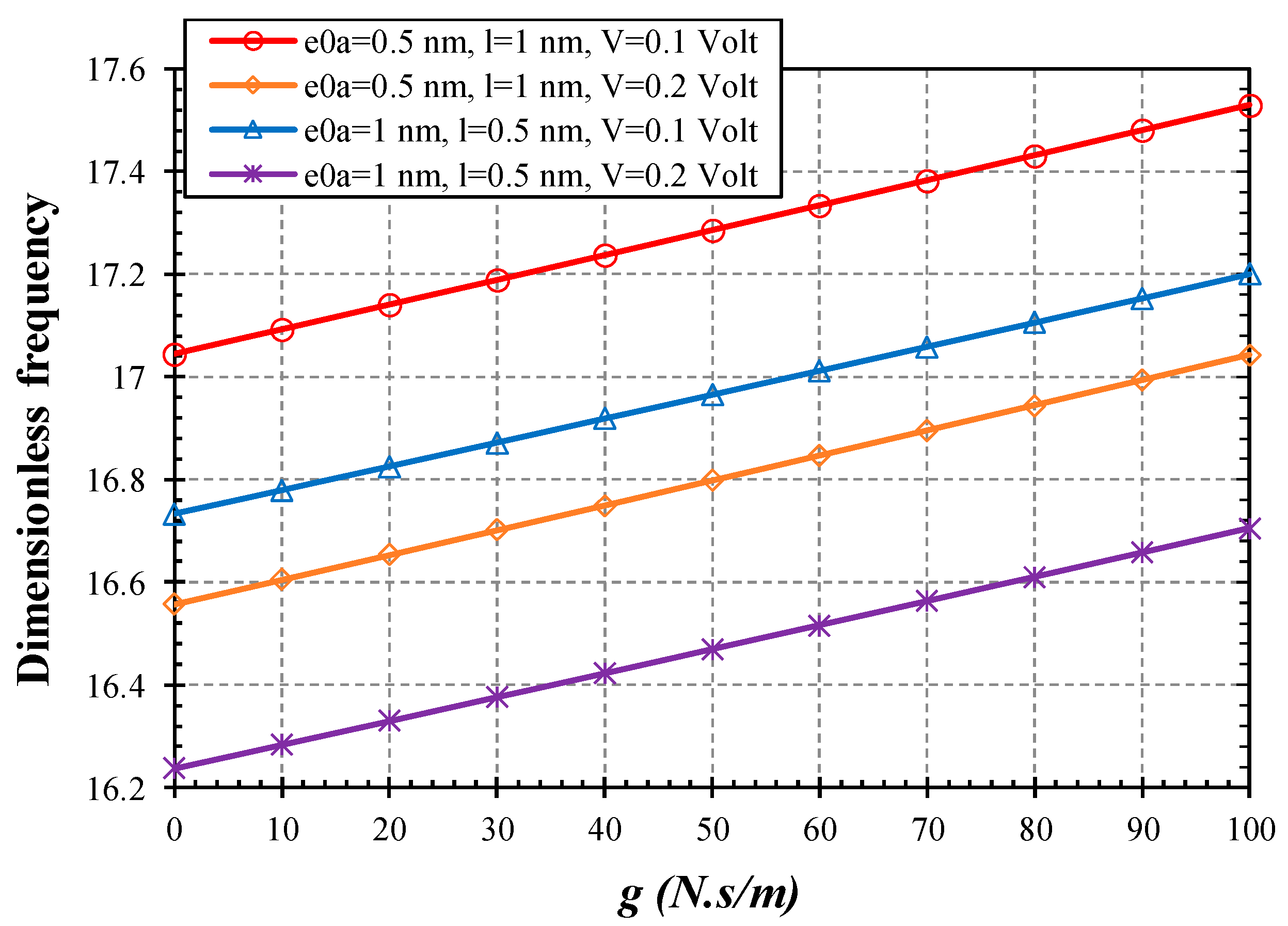
In terms of predicting the static and dynamic responses of piezoelectric–flexoelectric nanostructures, the previous published research studied many conditions, e.g., the effect of nonlocal parameter [29,34,38], different edge conditions [31], thermal environment [36], surface effect [36,37], elastic substrate [39], etc.; therefore, the present study focuses on the influence of flexoelectricity on a nanobeam with internal viscoelasticity. To this end, Figure 2 illustrates the variation in the viscoelastic parameter against changes in the nonlocal parameter and the upper surface voltage. According to the diagrams, there are two cases: when the SGLP is larger than the nonlocal parameter, and vice versa. The upper surface voltage is also taken in two values. As the figure shows, first, it should be stated that the larger the viscoelasticity, the greater the natural frequencies. On the other side, increasing the voltage results in a lower frequency. It can also be seen that l > e₀a produces larger frequencies compared to e₀a > l. Moreover, by looking carefully at the figure, it can be seen that the further decreasing impact of the voltage is related to the case e₀a > l.

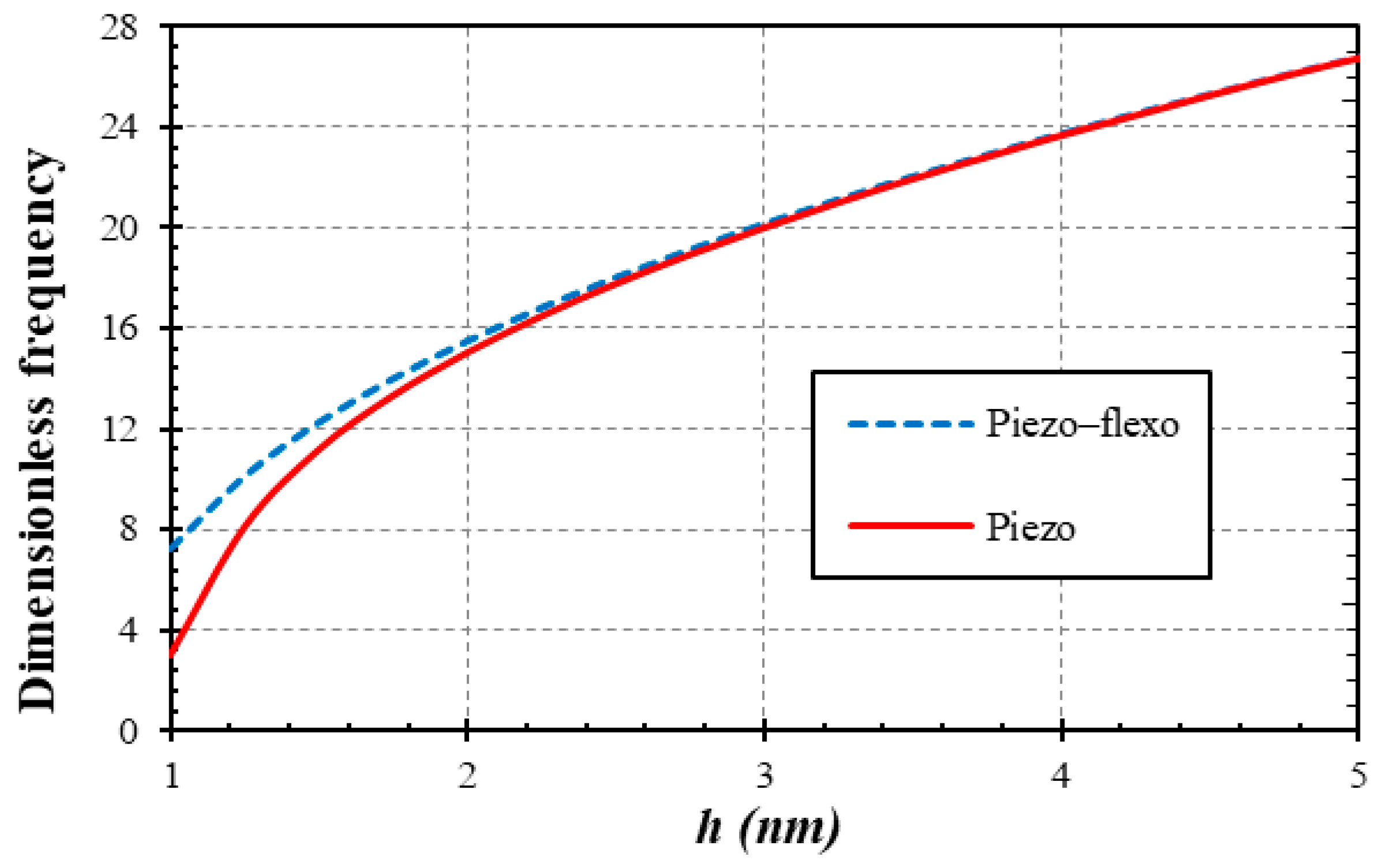
By means of Figure 3, one can make a simple comparison between the two states of the material: when we have only the piezo effect, and when we have both the piezo and flexo effects. It is worth mentioning that because polarization by flexoelectricity is far less than polarization with piezoelectricity, as flexoelectricity occurs due to the strain gradient and piezoelectricity happens due to strain itself, the piezo influence should be much greater than the flexo effect. Based on the figure, one can observe that the results of the case having both piezo and flexo impacts are more remarkable in smaller thicknesses compared to those neglecting the flexo effect. However, this figure proves that when the thickness of the nanobeam is sufficiently large, the effect of flexoelectricity is not noticeable.

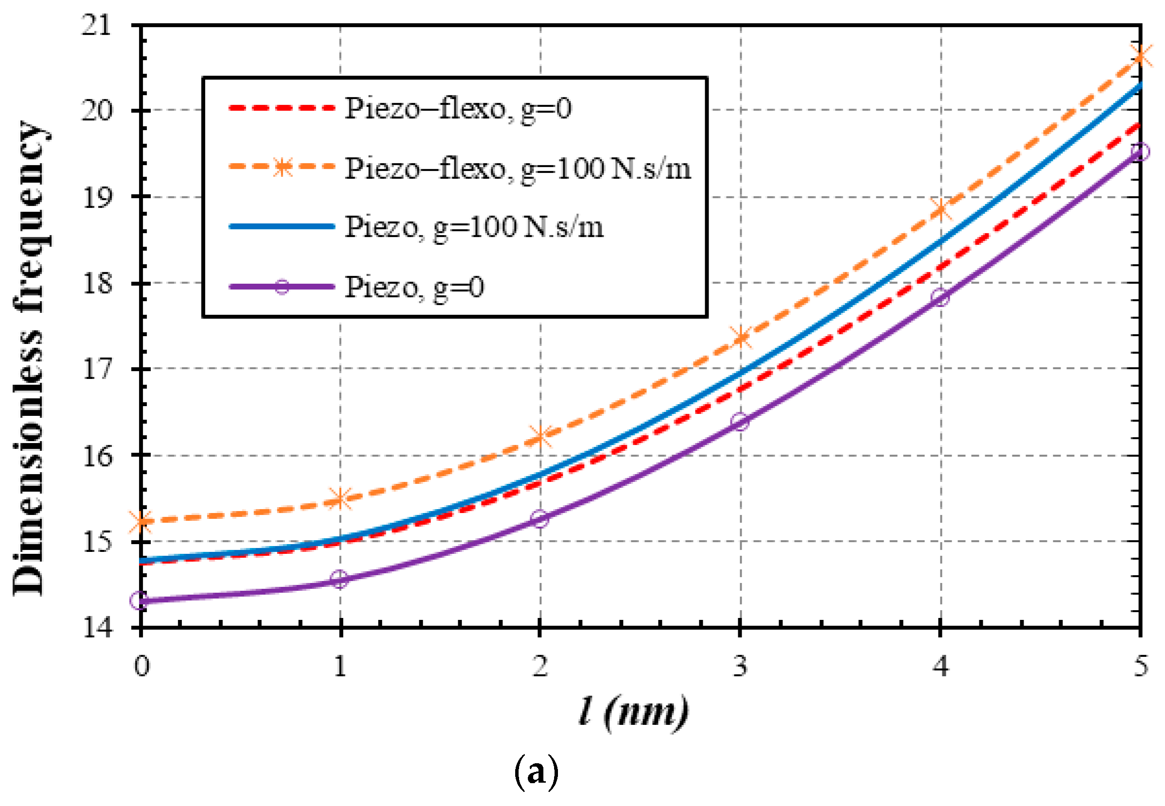
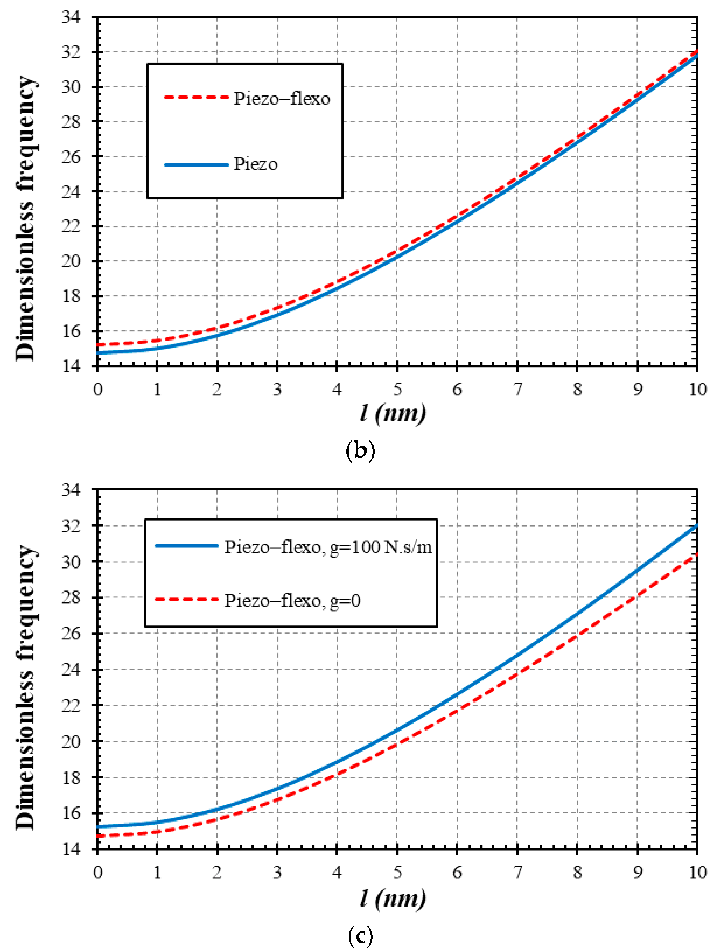
Figure 4a–c pictorially exhibits the variations of SGLP versus two states for the material, namely, that considering the internal viscoelasticity and that avoiding such a property for the piezoelectric and piezo–flexoelectric nanobeams. By reference to Figure 4a, one can see that by increasing the SGLP, the effect of flexoelectricity is subsequently reduced. It is clear mathematically that when g = 0 N.s/m or g = 100 N.s/m for both cases of material (piezo vs. piezo–flexo) and when the value of the gradient parameter is increased, the numerical results are closer to each other. This means that if the value of this parameter increases, the flexoelectricity effect is diminished. Thereby, on the basis of Figure 4b, one can obtain the conclusion of the previous figure. In this figure, the length scale quantity is further magnified (0 ≤ l ≤ 10 nm), and as can be observed, the results are inclined to be closer to each other. This is true for both piezo and piezo–flexo materials with an increase in the SGLP value. Furthermore, with regard to Figure 4c, for which greater values of gradient length scale factor were chosen and the piezo–flexo material was selected in two cases (with viscoelasticity and without it), one can see that the growth of the SGLP highlights the role of inner viscoelasticity. As a matter of fact, a sufficiently large value for length scale strain gradient parameter is very effective for analyzing internal viscoelastic coupling in a piezo–flexoelectric nanobeam exposed to dynamic conditions.

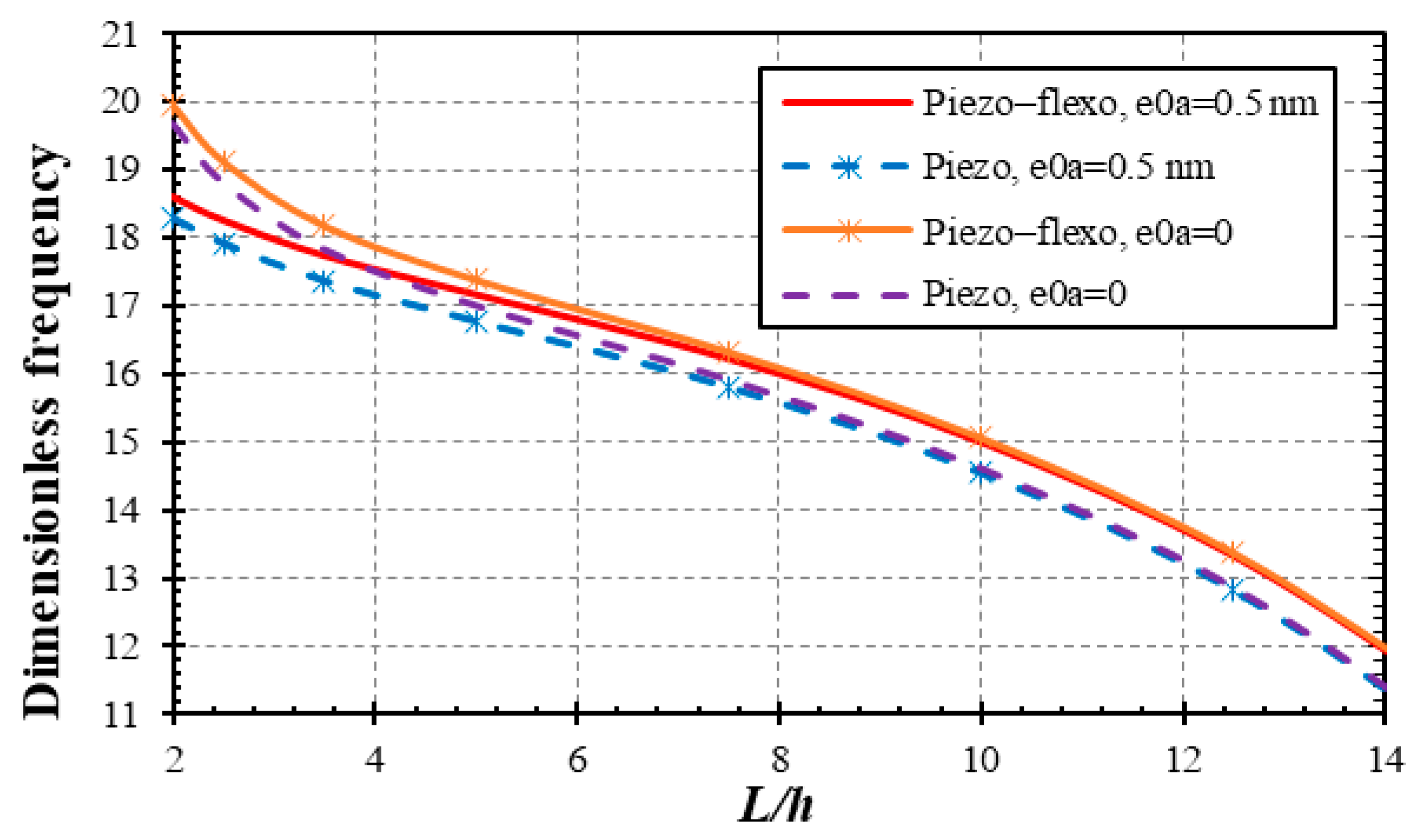
Figure 5 presents the role of larger lengths and their effect on the substance when it is piezo–flexo and when it is piezo only. In addition to these, the figure also contains different nonlocal parameters. With the help of the figure, one can see that an increase in the length-to-thickness ratio will result in a decline in the nonlocal parameter effect. This means that the results of cases piezo-e₀a = 0 and piezo-e₀a = 0.5 nm approach each other and are identical for large lengths. However, the most serious and marked result of this figure is the significance of flexoelectricity for larger lengths of the beam. Indeed, the results of piezo-e₀a = 0 versus piezo–flexo-e₀a = 0 and also piezo-e₀a = 0.5 nm versus piezo–flexo-e₀a = 0.5 nm become farther from one another after enlarging the length of the beam.

To provide further knowledge on the effect of viscoelasticity on flexoelectricity in a piezoelectric nanobeam, the mode shapes of frequency are here considered. The deformation resulting from frequency modes of beams is extremely small in an elastic condition (recoverable). To our knowledge, the Navier solution method is unable to give the deformations originating from eigenvalue problems and is only able to give values of natural frequencies. However, in a linear bending analysis and based on the static condensation, the Navier method can help to find linear deflections resulted from transverse loading. To plot the frequency mode shapes, we should solve the attained equation (Equation (41)). To this end, here, we employ an exact solution process. First, we should rewrite Equation (41) by simplifying it as

$$a\frac{d^{6}w}{d{x}^6}+b\frac{d^{4}w}{d{x}^4}+c\frac{d^{2}w}{d{x}^2}-j=0$$

(46)

in which

$$\begin{array}{l}a=-\mu \beta -l_{}^2\left[\gamma -C_{11}{I}_z\left(1-ig\omega \right)\right],\\ b=\beta +\mu \left({\omega }^2{I}_2-2d_{31}V\right)+\gamma -C_{11}{I}_z\left(1-ig\omega \right),\\ c=2d_{31}V-{\omega }^2\left(\mu I_0+I_2\right),\\ j=I_0{\omega }^2\cdot \end{array}$$

Equation (46) is a sixth-order ordinary differential equation, and we can guess an exponential solution form as follows.

$$w\left(x\right)=\exp (\lambda x)$$

(47)

Imposing Equation (47) on Equation (46), one can find a sextic equation as follows:

$$\left(a{\lambda }^6+b{\lambda }^4+c{\lambda }^2-j\right)\exp (\lambda x)=0$$

(48)

which implies a characteristic equation of

$$a{\lambda }^6+b{\lambda }^4+c{\lambda }^2-j=0.$$

Now the solution to Equation (46) will depend upon the solution to the above algebraic polynomial equation. If we suppose that all the roots for Equation (48) are real and distinct and ignore the imaginary part, we can guess the general solution for Equation (46) to be

$$w\left(x\right)={\displaystyle \sum _{i=1}^6{C}_i\exp ({\lambda }_{i}x)}$$

(49)

in which $C_i\left(i=1,\dots ,6\right)$ terms are the constants that should be determined based on the boundary conditions in Table 1.

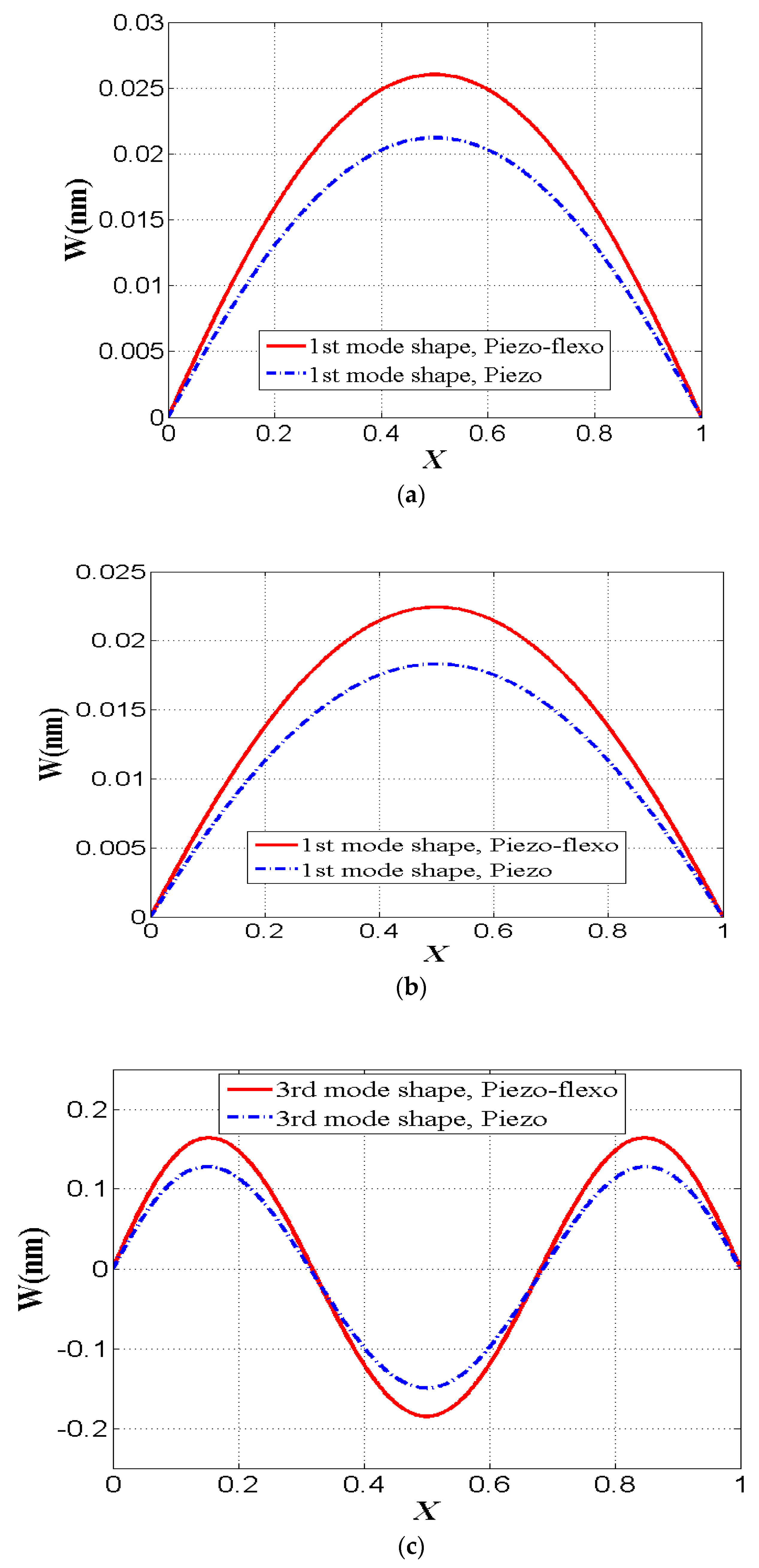
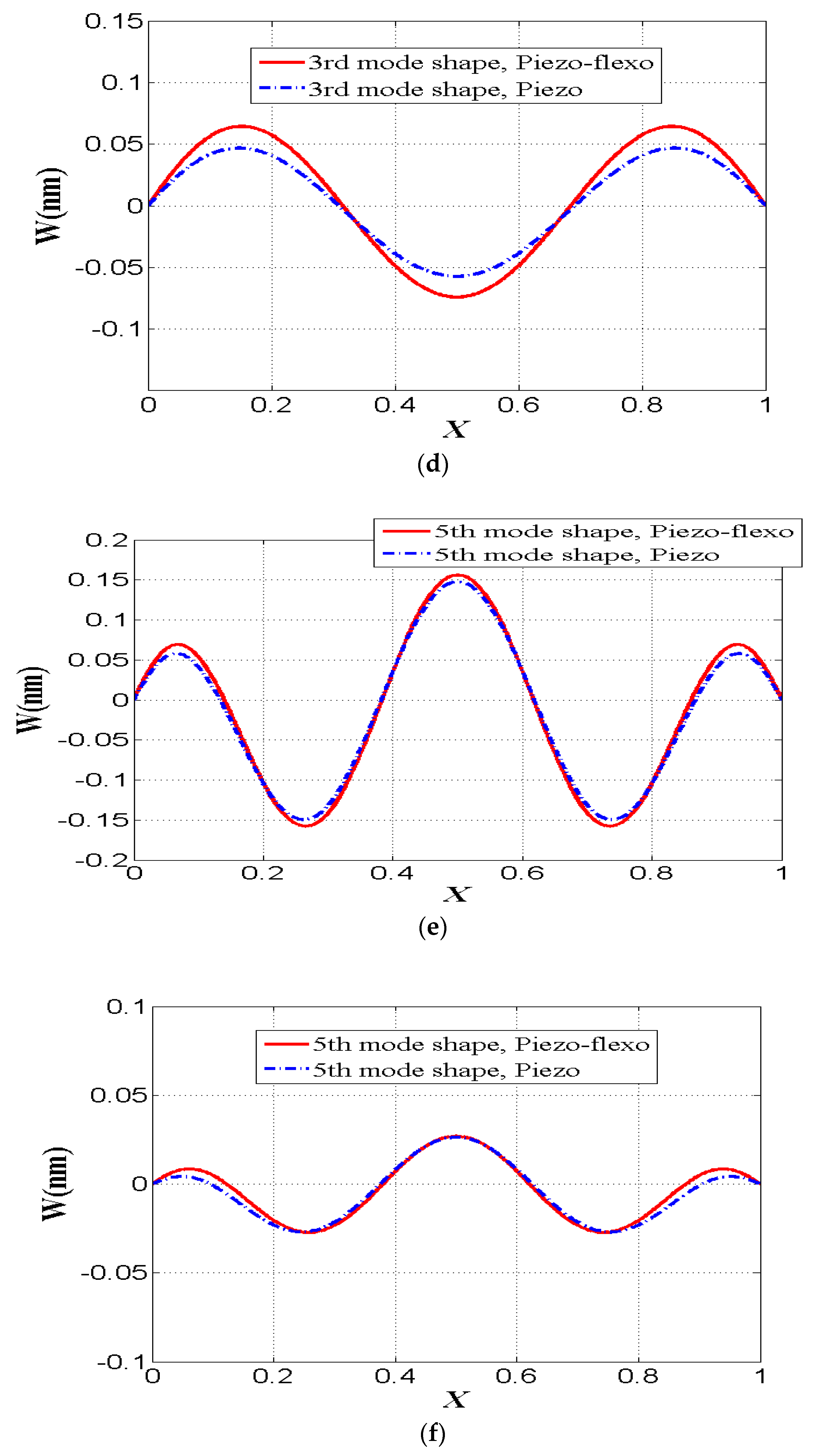
Now, in order to display the effect of inner viscoelasticity versus flexoelectricity, Figure 6a–f was plotted. This figure was drawn based on the mode shapes of nanobeams in two states; a piezo–flexoelectric nanobeam and a piezoelectric nanobeam. Figure 6a,b present the case of the first mode shape and Figure 6c,d show the third mode shape, and Figure 6e,f show the fifth mode shape. It should also be emphasized that only the real parts of the mode shapes are portrayed. For Figure 6a,c,e, the internal viscoelasticity is eliminated, and Figure 6b,d,f include the viscoelastic coupling by adopting g = 100 N.s/m. In Figure 6b,d,f, the percent difference of the results of the two kinds of materials is greater than that in Figure 6a,c,e. For example, for Figure 6c, W_PF/W_P = 1.238, while for Figure 6d, W_PF/W_P = 1.293. In other words, when a material, in addition to piezoelectricity, also includes the flexoelectricity effect, it is further affected by the internal damping. In addition, this conclusion was observed to be clearer for higher mode shapes. Furthermore, it is worth noting that whenever the viscoelastic parameter’s value increased, the deflections decreased. Moreover, as flexoelectricity makes the material more flexible, the deflection by a piezo–flexoelectric nanomaterial would be higher than that by a piezoelectric one. It should be pointed out that all the mode shapes are symmetric. Consequently, these diagrams convey the noteworthy finding that a higher inner viscoelasticity parameter value strengthens the role of flexoelectricity in the nanomaterial.

6. Conclusions

This research, for the first time, incorporated viscoelasticity into a piezoelectric–flexoelectric Euler–Bernoulli nanobeam, while Kelvin–Voigt linear viscoelastic coupling was applied to the dynamic analysis. To convert achieved dynamic equations to nano size, an effective way can be to use nonlocal continuum theories. Hence, this paper was concerned with the use of a nonlocal model based on the second strain and stress gradients. The boundary condition taken into consideration was pivot–pivot on the basis of an analytical approach. The mode shapes, for the first time, were drawn for a piezoelectric nanobeam, while NSGT contributed. We produced some substantial findings, as given below.

∗

The smaller the thickness, the larger the impact of flexoelectricity.

∗

The lesser the SGLP values, the greater the flexoelectric effect.

∗

The larger the length of the nanobeam, the larger the influence of flexoelectricity.

∗

The greater the inner viscoelastic values, the greater the role of flexoelectricity.

∗

The larger the SGLP values, the greater the inner viscoelastic impact.

∗

The higher the mode number, the larger the influence of flexoelectricity.

References

- Ma, W. Flexoelectricity: Strain gradient effects in ferroelectrics. Phys. Scripta 2007, T129, 180–183. [Google Scholar] [CrossRef]
- Lee, D.; Yoon, A.; Jang, S.Y.; Yoon, J.-G.; Chung, J.-S.; Kim, M.; Scott, J.F.; Noh, T.W. Giant Flexoelectric Effect in Ferroelectric Epitaxial Thin Films. Phys. Rev. Lett. 2011, 107, 057602. [Google Scholar] [CrossRef] [PubMed]
- Nguyen, T.D.; Mao, S.; Yeh, Y.-W.; Purohit, P.K.; McAlpine, M.C. Nanoscale Flexoelectricity. Adv. Mater. 2013, 25, 946–974. [Google Scholar] [CrossRef] [PubMed]
- Zubko, P.; Catalan, G.; Tagantsev, A.K. Flexoelectric Effect in Solids. Ann. Rev. Mater. Res. 2013, 43, 387–421. [Google Scholar] [CrossRef] [Green Version]
- Yudin, P.V.; Tagantsev, A.K. Fundamentals of flexoelectricity in solids. Nanotechnology 2013, 24, 432001. [Google Scholar] [CrossRef]
- Jiang, X.; Huang, W.; Zhang, S. Tagantsev, A.K. Flexoelectric nano-generators: Materials, structures and devices. Nano Energy 2013, 2, 1079–1092. [Google Scholar] [CrossRef]
- Yurkov, A.S.; Tagantsev, A.K. Strong surface effect on direct bulk flexoelectric response in solids. Appl. Phys. Lett. 2016, 108, 022904. [Google Scholar] [CrossRef]
- Wang, B.; Gu, Y.; Zhang, S.; Chen, L.-Q. Flexoelectricity in solids: Progress, challenges, and perspectives. Prog. Mater. Sci. 2019, 106, 100570. [Google Scholar] [CrossRef]
- Cross, L. Flexoelectric effects: Charge separation in insulating solids subjected to elastic strain gradients. J. Mater. Sci. 2006, 41, 53–63. [Google Scholar] [CrossRef]
- Ma, W.; Cross, L.E. Observation of the flexoelectric effect in relaxor Pb (Mg1/3Nb2/3)O3 ceramics. Appl. Phys. Lett. 2001, 78, 2920–2921. [Google Scholar] [CrossRef]
- Ma, W.; Cross, L.E. Flexoelectricity of barium titanate. Appl. Phys. Lett. 2006, 88, 232902. [Google Scholar] [CrossRef]
- Zubko, P.; Catalan, G.; Buckley, A.; Welche, P.R.L.; Scott, J.F. Strain-gradient-induced polarization in SrTiO3 single crystals. Phys. Rev. Lett. 2007, 99, 167601. [Google Scholar] [CrossRef] [PubMed] [Green Version]
- Eremeyev, V.A.; Ganghoffer, J.-F.; Konopinska-Zmysłowska, V.; Uglov, N.S. Flexoelectricity and apparent piezoelectricity of a pantographic micro-bar. Int. J. Eng. Sci. 2020, 149, 103213. [Google Scholar] [CrossRef]
- Malikan, M. Electro-mechanical shear buckling of piezoelectric nanoplate using modified couple stress theory based on simplified first order shear deformation theory. Appl. Math. Model. 2017, 48, 196–207. [Google Scholar] [CrossRef]
- Malikan, M. Temperature influences on shear stability of a nanosize plate with piezoelectricity effect. Multidiscip. Model. Mater. Struct. 2018, 14, 125–142. [Google Scholar] [CrossRef]
- Malikan, M. Electro-thermal buckling of elastically supported double-layered piezoelectric nanoplates affected by an external electric voltage. Multidiscip. Model. Mater. Struct. 2019, 15, 50–78. [Google Scholar] [CrossRef]
- Liu, C.; Kea, L.-L.; Yang, J.; Kitipornchaic, S.; Wang, Y.-S. Buckling and post-buckling analyses of size-dependent piezoelectric nanoplates. Theor. Appl. Mech. Lett. 2016, 6, 253–267. [Google Scholar] [CrossRef] [Green Version]
- Ansari, R.; Faraji Oskouiea, M.; Gholami, R.; Sadegh, F. Thermo-electro-mechanical vibration of postbuckled piezoelectric Timoshenko nanobeams based on the nonlocal elasticity theory. Compos. Part B Eng. 2016, 89, 316–327. [Google Scholar] [CrossRef]
- Tadi Beni, Y. Size-dependent analysis of piezoelectric nanobeams including electro-mechanical coupling. Mech. Res. Commun. 2016, 75, 67–80. [Google Scholar] [CrossRef]
- Malekzadeh Fard, K.; Khajehdehi Kavanroodi, M.; Malek-Mohammadi, H.; Pourmoayed, A. Buckling and vibration analysis of a double-layer Graphene sheet coupled with a piezoelectric nanoplate. J. Appl. Comput. Mech. 2020. [Google Scholar] [CrossRef]
- Craciun, E.M.; Baesu, E.; Soós, E. General solution in terms of complex potentials for incremental antiplane states in prestressed and prepolarized piezoelectric crystals: Application to Mode III fracture propagation. IMA J. Appl. Math. 2004, 70, 39–52. [Google Scholar] [CrossRef]
- Palacios, A.; In, V.; Longhini, P. Symmetry-Breaking as a Paradigm to Design Highly-Sensitive Sensor Systems. Symmetry 2015, 7, 1122–1150. [Google Scholar] [CrossRef] [Green Version]
- Karami, B.; Shahsavari, D.; Li, L.; Karami, M.; Janghorban, M. Thermal buckling of embedded sandwich piezoelectric nanoplates with functionally graded core by a nonlocal second-order shear deformation theory. Proc. Inst. Mech. Eng. C-J. Mech. Eng. Sci. 2019, 233, 287–301. [Google Scholar] [CrossRef]
- Liang, X.; Hu, S.; Shen, S. Effects of surface and flexoelectricity on a piezoelectric nanobeam. Smart Mater. Struct. 2014, 23, 035020. [Google Scholar] [CrossRef]
- Zhang, R.; Liang, X.; Shen, S. A Timoshenko dielectric beam model with flexoelectric effect. Meccanica 2016, 51, 1181–1188. [Google Scholar] [CrossRef]
- Qi, L.; Zhou, S.; Li, A. Size-dependent bending of an electro-elastic bilayer nanobeam due to flexoelectricity and strain gradient elastic effect. Compos. Struct. 2016, 135, 167–175. [Google Scholar] [CrossRef]
- Sneha Rupa, N.; Ray, M.C. Analysis of flexoelectric response in nanobeams using nonlocal theory of elasticity. Int. J. Mech. Mater. Des. 2017, 13, 453–467. [Google Scholar] [CrossRef]
- Xiang, S.; Li, X.-F. Elasticity solution of the bending of beams with the flexoelectric and piezoelectric effects. Smart Mater. Struct. 2018, 27, 105023. [Google Scholar] [CrossRef]
- Zarepour, M.; Hosseini, S.A.H.; Akbarzadeh, A.H. Geometrically nonlinear analysis of Timoshenko piezoelectric nanobeams with flexoelectricity effect based on Eringen’s differential model. Appl. Math. Model. 2019, 69, 563–582. [Google Scholar] [CrossRef]
- Yang, X.; Zhou, Y.; Wang, B.; Zhang, B. A finite-element method of flexoelectric effects on nanoscale beam. Int. J. Multiscale Comp. 2019, 17, 29–43. [Google Scholar] [CrossRef]
- Zhao, X.; Zheng, S.; Li, Z. Size-dependent nonlinear bending and vibration of flexoelectric nanobeam based on strain gradient theory. Smart Mater. Struct. 2019, 28, 075027. [Google Scholar] [CrossRef]
- Basutkar, R.; Sidhardh, S.; Ray, M.C. Static analysis of flexoelectric nanobeams incorporating surface effects using element free Galerkin method. Eur. J. Mech. A-Solid 2019, 76, 13–24. [Google Scholar] [CrossRef]
- Ghobadi, A.; Tadi Beni, Y.; Golestanian, H. Size dependent thermo-electro-mechanical nonlinear bending analysis of flexoelectric nano-plate in the presence of magnetic field. Int. J. Mech. Sci. 2019, 152, 118–137. [Google Scholar] [CrossRef]
- Ebrahimi, F.; Karimiasl, M. Nonlocal and surface effects on the buckling behavior of flexoelectric sandwich nanobeams. Mech. Adv. Mater. Struct. 2018, 25, 943–952. [Google Scholar] [CrossRef]
- Zeng, S.; Wang, B.L.; Wang, K.F. Static stability analysis of nanoscale piezoelectric shells with flexoelectric effect based on couple stress theory. Microsyst. Technol. 2018, 24, 2957–2967. [Google Scholar] [CrossRef]
- Barati, M.R. On non-linear vibrations of flexoelectric nanobeams. Int. J. Eng. Sci. 2017, 121, 143–153. [Google Scholar] [CrossRef]
- Arefi, M.; Pourjamshidian, M.; Ghorbanpour Arani, A.; Rabczuk, T. Influence of flexoelectric, small-scale, surface and residual stress on the nonlinear vibration of sigmoid, exponential and power-law FG Timoshenko nano-beams. J. Low Freq. Noise Vib. Act. Control 2019, 38, 122–142. [Google Scholar] [CrossRef] [Green Version]
- Ebrahimi, F.; Barati, M.R. Surface effects on the vibration behavior of flexoelectric nanobeams based on nonlocal elasticity theory. Eur. Phys. J. Plus 2017, 132, 19. [Google Scholar] [CrossRef]
- Amiri, A.; Vesal, R.; Talebitooti, R. Flexoelectric and surface effects on size-dependent flow-induced vibration and instability analysis of fluid-conveying nanotubes based on flexoelectricity beam model. Int. J. Mech. Sci. 2019, 156, 474–485. [Google Scholar] [CrossRef]
- Parsa, A.; Mahmoudpour, E. Nonlinear free vibration analysis of embedded flexoelectric curved nanobeams conveying fluid and submerged in fluid via nonlocal strain gradient elasticity theory. Microsyst. Technol. 2019, 25, 4323–4339. [Google Scholar] [CrossRef]
- Vaghefpour, H.; Arvin, H. Nonlinear free vibration analysis of pre-actuated isotropic piezoelectric cantilever Nano-beams. Microsyst. Technol. 2019, 25, 4097–4110. [Google Scholar] [CrossRef]
- Fattahian Dehkordi, S.; Tadi Beni, Y. Electro-mechanical free vibration of single-walled piezoelectric/flexoelectric nano cones using consistent couple stress theory. Int. J. Mech. Sci. 2017, 128–129, 125–139. [Google Scholar] [CrossRef]
- Joseph, R.P.; Zhang, C.; Wang, B.L. Samali, Fracture analysis of flexoelectric double cantilever beams based on the strain gradient theory. Compos. Struct. 2018, 202, 1322–1329. [Google Scholar] [CrossRef]
- Malikan, M.; Dimitri, R.; Tornabene, F. Transient response of oscillated carbon nanotubes with an internal and external damping. Compos. Part B Eng. 2019, 158, 198–205. [Google Scholar] [CrossRef]
- Jalaei, M.H.; Civalek, Ö. On dynamic instability of magnetically embedded viscoelastic porous FG nanobeam. Int. J. Eng. Sci. 2019, 143, 14–32. [Google Scholar] [CrossRef]
- Ebrahimi, F.; Barati, M.R. Hygrothermal effects on vibration characteristics of viscoelastic FG nanobeams based on nonlocal strain gradient theory. Compos. Struct. 2017, 159, 433–444. [Google Scholar] [CrossRef]
- Li, C.; Liu, J.J.; Cheng, M.; Fan, X.L. Nonlocal vibrations and stabilities in parametric resonance of axially moving viscoelastic piezoelectric nanoplate subjected to thermo-electro-mechanical forces. Compos. Part B Eng. 2017, 116, 153–169. [Google Scholar] [CrossRef]
- Zenkour, A.M.; Sobhy, M. Nonlocal piezo-hygrothermal analysis for vibration characteristics of a piezoelectric Kelvin–Voigt viscoelastic nanoplate embedded in a viscoelastic medium. Acta Mech. 2018, 229, 3–19. [Google Scholar] [CrossRef]
- Tadi Beni, Z.; Hosseini Ravandi, S.A.; Tadi Beni, Y. Size-dependent nonlinear forced vibration analysis of viscoelastic/piezoelectric nano-beam. J. Appl. Comput. Mech. 2020. [Google Scholar] [CrossRef]
- Argatov, I.; Butcher, E.A. On the separation of internal and boundary damage in slender bars using longitudinal vibration frequencies and equivalent linearization of damaged bolted joint response. J. Sound Vib. 2011, 330, 3245–3256. [Google Scholar] [CrossRef]
- Qiao, G.; Rahmatallah, S. Identification of the viscoelastic boundary conditions of Euler-Bernoulli beams using transmissibility. Eng. Rep. 2019, 1, e12074. [Google Scholar] [CrossRef]
- Song, X.; Li, S.-R. Thermal buckling and post-buckling of pinned–fixed Euler–Bernoulli beams on an elastic foundation. Mech. Res. Commun. 2007, 34, 164–171. [Google Scholar] [CrossRef]
- Reddy, J.N. Nonlocal nonlinear formulations for bending of classical and shear deformation theories of beams and plates. Int. J. Eng. Sci. 2010, 48, 1507–1518. [Google Scholar] [CrossRef]
- Lim, C.W.; Zhang, G.; Reddy, J.N. A Higher-order nonlocal elasticity and strain gradient theory and Its Applications in wave propagation. J. Mech. Phys. Solids 2015, 78, 298–313. [Google Scholar] [CrossRef]
- Ansari, R.; Sahmani, S.; Arash, B. Nonlocal plate model for free vibrations of single-layered graphene sheets. Phys. Lett. A 2010, 375, 53–62. [Google Scholar] [CrossRef]
- Akbarzadeh Khorshidi, M. The material length scale parameter used in couple stress theories is not a material constant. Int. J. Eng. Sci. 2018, 133, 15–25. [Google Scholar] [CrossRef]
- Malikan, M.; Nguyen, V.B.; Dimitri, R.; Tornabene, F. Dynamic modeling of non-cylindrical curved viscoelastic single-walled carbon nanotubes based on the second gradient theory. Mater. Res. Express 2019, 6, 075041. [Google Scholar] [CrossRef]
- Malikan, M.; Nguyen, V.B. Buckling analysis of piezo-magnetoelectric nanoplates in hygrothermal environment based on a novel one variable plate theory combining with higher-order nonlocal strain gradient theory. Phys. E 2018, 102, 8–28. [Google Scholar] [CrossRef]
- Malikan, M.; Krasheninnikov, M.; Eremeyev, V.A. Torsional stability capacity of a nano-composite shell based on a nonlocal strain gradient shell model under a three-dimensional magnetic field. Int. J. Eng. Sci. 2020, 148, 103210. [Google Scholar] [CrossRef]
- Malikan, M.; Eremeyev, V.A. Post-critical buckling of truncated conical carbon nanotubes considering surface effects embedding in a nonlinear Winkler substrate using the Rayleigh-Ritz method. Mater. Res. Express 2020, 7, 025005. [Google Scholar] [CrossRef]
- Malikan, M. On the plastic buckling of curved carbon nanotubes. Theor. Appl. Mech. Lett. 2020, 10, 46–56. [Google Scholar] [CrossRef]
- Malikan, M.; Nguyen, V.B.; Tornabene, F. Electromagnetic forced vibrations of composite nanoplates using nonlocal strain gradient theory. Mater. Res. Express 2018, 5, 075031. [Google Scholar] [CrossRef]
- Lei, Y.; Adhikari, S.; Friswell, M.I. Vibration of nonlocal Kelvin–Voigt viscoelastic damped Timoshenko beams. Int. J. Eng. Sci. 2013, 66–67, 1–13. [Google Scholar] [CrossRef]
- Liu, H.; Liu, H.; Yang, J. Vibration of FG magneto-electro-viscoelastic porous nanobeams on visco-Pasternak foundation. Compos. Part B Eng. 2018, 155, 244–256. [Google Scholar] [CrossRef]
- Malikan, M.; Dimitri, R.; Tornabene, F. Effect of sinusoidal corrugated geometries on the vibrational response of viscoelastic nanoplates. Appl. Sci. 2018, 8, 1432. [Google Scholar] [CrossRef] [Green Version]
- Soltani, P.; Kassaei, A.; Taherian, M.M. Nonlinear and quasi-linear behavior of a curved carbon nanotube vibrating in an electric force field; analytical approach. Acta Mech. Solida Sin. 2014, 27, 97–110. [Google Scholar] [CrossRef]
- Zare Jouneghani, F.; Dimitri, R.; Tornabene, F. Structural response of porous FG nanobeams under hygro thermo-mechanical loadings. Compos. Part B Eng. 2018, 152, 71–78. [Google Scholar] [CrossRef]
- Lu, L.; Guo, X.; Zhao, J. Size-dependent vibration analysis of nanobeams based on the nonlocal strain gradient theory. Int. J. Eng. Sci. 2017, 116, 12–24. [Google Scholar] [CrossRef]
- Mehralian, F.; Tadi Beni, Y.; Karimi Zeverdejani, M. Nonlocal strain gradient theory calibration using molecular dynamics simulation based on small scale vibration of nanotubes. Phys. B 2017, 514, 61–69. [Google Scholar] [CrossRef]
- Malikan, M.; Nguyen, V.B.; Tornabene, F. Damped forced vibration analysis of single-walled carbon nanotubes resting on viscoelastic foundation in thermal environment using nonlocal strain gradient theory. Eng. Sci. Technol. Int. J. 2018, 21, 778–786. [Google Scholar] [CrossRef]
- Yang, W.; Liang, X.; Shen, S. Electromechanical responses of piezoelectric nanoplates with flexoelectricity. Acta Mech. 2015, 226, 3097–3110. [Google Scholar] [CrossRef]
- Ansari, R.; Sahmani, S.; Rouhi, H. Rayleigh–Ritz axial buckling analysis of single-walled carbon nanotubes with different boundary conditions. Phys. Lett. A 2011, 375, 1255–1263. [Google Scholar] [CrossRef]
- Duan, W.H.; Wang, C.M. Exact solutions for axisymmetric bending of micro/nanoscale circular plates based on nonlocal plate theory. Nanotechnology 2007, 18, 385704. [Google Scholar] [CrossRef]
- Duan, W.H.; Wang, C.M.; Zhang, Y.Y. Calibration of nonlocal scaling effect parameter for free vibration of carbon nanotubes by molecular dynamics. J. Appl. Phys. 2007, 101, 24305. [Google Scholar] [CrossRef]
Figure 1.
A dielectric hinged–hinged nanobeam’s configuration (designed in a CAD program (SolidWorks)).
Figure 2.
Viscoelastic parameter vs. small-scale parameters and the effects of voltage on the nondimensional natural frequency (L = 10h, h = 2 nm).
Figure 3.
Thickness parameter vs. flexoelectricity effect on the nondimensional natural frequency (e0a = 0.5 nm, l = 1 nm, V = 0.5 Volt, L = 10h, g = 100 N.s/m).
Figure 4.
(a) Strain gradient length scale parameter vs. flexoelectricity effect and viscoelastic parameter effect on the nondimensional natural frequency (e0a = 0.5 nm, h = 2 nm, L = 10h, V = 0.5 Volt). (b) Strain gradient length scale parameter vs. flexoelectricity effect on the nondimensional natural frequency (e0a = 0.5 nm, h = 2 nm, L = 10h, V = 0.5 Volt, g = 100 N.s/m). (c) Strain gradient length scale parameter vs. viscoelastic effect on the nondimensional natural frequency (e0a = 0.5 nm, h = 2 nm, L = 10h, V = 0.5 Volt).
Figure 5.
Length-to-thickness ratio vs. flexoelectricity effect on the nondimensional natural frequency (l = 1 nm, h = 2 nm, V = 0.5 Volt, g = 0 N.s/m).
Figure 6.
(a) First mode shape for two cases: the presence of flexoelectricity and its absence without inner damping (e0a = 0.5 nm, l = 1 nm, h = 2 nm, V = 0.5 Volt, g = 0 N.s/m). (b) First mode shape for two cases: the presence of flexoelectricity and its absence including internal viscoelasticity (e0a = 0.5 nm, l = 1 nm, h = 2 nm, V = 0.5 Volt, g = 100 N.s/m). (c) Third mode shape for two cases: the presence of flexoelectricity and its absence without inner damping (e0a = 0.5 nm, l = 1 nm, h = 2 nm, V = 0.5 Volt, g = 0 N.s/m). (d) Third mode shape for two cases: the presence of flexoelectricity and its absence with inner damping (e0a = 0.5 nm, l = 1 nm, h = 2 nm, V = 0.5 Volt, g = 100 N.s/m). (e) Fifth mode shape for two cases: the presence of flexoelectricity and its absence without inner damping (e0a = 0.5 nm, l = 1 nm, h = 2 nm, V = 0.5 Volt, g = 0 N.s/m). (f) Fifth mode shape for two cases: the presence of flexoelectricity and its absence with inner damping (e0a = 0.5 nm, l = 1 nm, h = 2 nm, V = 0.5 Volt, g = 100 N.s/m).