The Generalized Gielis Geometric Equation and Its Application


1
Bamboo Research Institute, College of Biology and the Environment, Nanjing Forestry University, Nanjing 210037, China
2
Tasmanian Institute of Agriculture, University of Tasmania, Private Bag 98, Hobart 7001, Australia
3
Department of Biosciences Engineering, University of Antwerp, B-2020 Antwerp, Belgium
*
Author to whom correspondence should be addressed.
Symmetry 2020, 12(4), 645; https://0-doi-org.brum.beds.ac.uk/10.3390/sym12040645
Submission received: 28 March 2020
/
Revised: 15 April 2020
/
Accepted: 15 April 2020
/
Published: 17 April 2020
Abstract
:Many natural shapes exhibit surprising symmetry and can be described by the Gielis equation, which has several classical geometric equations (for example, the circle, ellipse and superellipse) as special cases. However, the original Gielis equation cannot reflect some diverse shapes due to limitations of its power-law hypothesis. In the present study, we propose a generalized version by introducing a link function. Thus, the original Gielis equation can be deemed to be a special case of the generalized Gielis equation (GGE) with a power-law link function. The link function can be based on the morphological features of different objects so that the GGE is more flexible in fitting the data of the shape than its original version. The GGE is shown to be valid in depicting the shapes of some starfish and plant leaves.
1. Introduction
In geometry, the equation of a circle in the Euclidean plane is usually expressed as
where x and y are the coordinates of the circle on the x- and y-axes, respectively, with r the radius. The circle is a special case of that of an ellipse:
where A and B (A ≥ B > 0) represent the major and minor axis semi-diameters, respectively. Interestingly, circles and ellipses, as well as squares and rectangles, can be regarded as special cases of Lamé curves [1,2], whose mathematical expression is listed as
where n is a real number. This equation has been shown to be valid for describing the actual cross-sections of tree rings and bamboo shoots [2,3,4,5]. Equation (3) in polar coordinates can be rewritten as
where r and ϕ are the polar radius and the angle between the straight line where the polar radius lies and the x-axis, respectively.
Gielis proposed a more general polar equation that can reflect more complex natural shapes [1,2]:
where n1, n2 and n3 are constants (both ); positive integer m was introduced to make the curve generate arbitrary polygons (with m angles) consequently enhancing the flexibility of Lamé curves. We refer to Equation (5) as the original Gielis equation (OGE) in the following text for simplicity. OGE has been used to simulate many natural shapes, e.g., diatoms, eggs, cross sections of plants, snowflakes and starfish [1,2]. OGE also has shown its validity in describing several actual natural shapes, e.g., leaf shapes of Hydrocotyle vulgaris L., Polygonum perfoliatum L. and seed planar projections of Ginkgo biloba L. [6,7]. Furthermore, OGE can produce regular, or at least very approximately regular polygons [8,9]. When m = 1, A = B, n1 = n, and n2 = n3 = 1, OGE has a special case:
where . This simplified version has been used to describe the actual leaf shapes of 46 bamboo species [2,10,11].
Although OGE is rather flexible in fitting the edge data of many natural shapes, it sometimes fails to describe accurately some symmetrical natural shapes. To further strengthen its flexibility of data fitting, we attempt to build a more generalized equation based on OGE, motivated by the study of starfish, which display a wide diversity of shapes, not only the archetypical shapes. In the Plateau problem of minimal surfaces, one of the constant mean curvature solutions for a soap film is a sphere, but these solutions are for isotropic energy distributions only.
In crystallography, Wulff shapes describe anisotropic distributions of energy, and can take many forms, with their corresponding constant anisotropic mean curvature surfaces [12]. Extending this principle to biological species, starfish can be considered as spheres for specific anisotropic energy distributions. Remarkably, pincushion starfish of the genus Culcita are close to spherical, intermediate between classical spheres and the archetypical shapes of five-armed starfish. Another notable group of starfish are biscuit starfish, almost pentagonal and flat. They belong to the genus Tosia. In order to apply the above methods to these groups, a modification of the original Gielis equation is necessary.
2. The Generalized Gielis Equation (GGE) and Its Two New Special Cases
OGE can be rewritten as [6]
where , and . Consider the formula inside the parentheses of Equation (7), which we define as follows:
We refer to this as the elementary Gielis equation (EGE) for convenience. OGE hypothesizes the existence of a power-law relationship between r and re. We refer to this relationship as the link function, f. As this link function can take on other forms, we use the following more general expression to replace OGE:
which we refer to as the generalized Gielis equation (GGE). In actuality, re is the polar radius of the elementary Gielis curve generated by EGE, and r is the polar radius of the generalized Gielis curve generated by GGE. Therefore, OGE is actually a special case of GGE with a power-law link function.
In the current study, we propose the following two candidate forms of the link function:
and
If we use the log transformation for the left-and right-hand sides of the above two equations, we obtain, respectively:
and
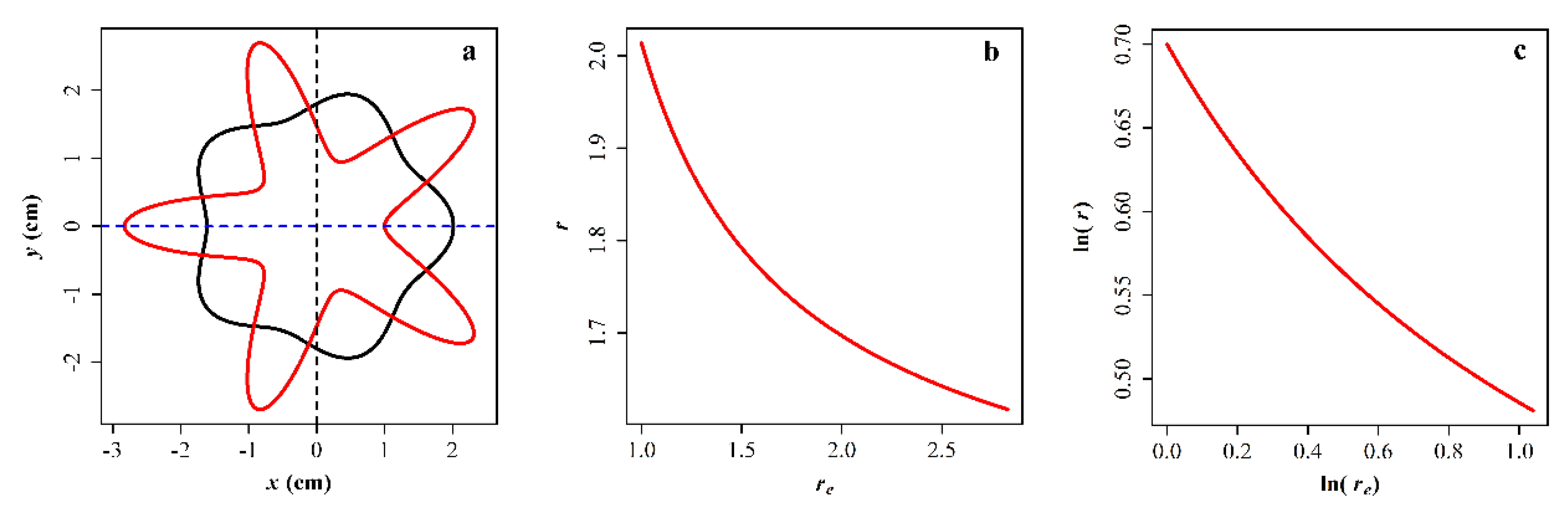
where and . The first equation is actually a hyperbolic equation, and the second one is a quadratic equation. If we also use the log transformation for both sides of the power-law link function in OGE, a linear equation is obtained. We can express that by letting the coefficient δ2 in Equation (13) be zero. Of course, in nature, there are forms other than the above link functions; however, these other forms also belong to the scope of GGE if there exists a clear functional expression between r and re. Figure 1 provides a simulation example for Equation (10).
3. Application of the Generalized Gielis Equation
In this section, we mainly illustrate the application of GGE to several starfish species of the families Goniasteridae and Oreasteridae. Culcita and Tosia are the target genera, and Anthenoides tenuis and Stellaster equestris are used as long-armed reference species. Furthermore, we test this on the leaves of four plant species; in particular, we test whether this extension is applicable to elliptical leaves with a broad basis. Table A1 in Appendix A shows the source of the material and species information.
Considering that the five arms of the starfish in Goniasteridae and Oreasteridae are approximately equal, we further simplify Equation (8) to
For starfish, we fix m to be 5; for leaves, we fix m to be 1. To measure the goodness of fit, root-mean-square error (RMSE) is used:
where and represent the observed and predicted polar radii of a starfish or a leaf described by GGE; N represents the number of data points on the edge of that starfish or that leaf. In fact, , where RSS is the residual sum of squares. However, RMSE is not suitable for comparing the goodness of fit among different samples. The reason is that a large object usually has a larger RMSE than a small object even when the fit to the former is just as good. Thus, we use the following adjusted RMSE (RMSEadj) that can reduce the influence of the object’s size [13]:
where A represents the area of an object of interest. We do not use the coefficient of determination (i.e., r2) as an indicator because it has been considered to be problematic for reflecting the goodness of fit of a nonlinear regression [14,15].
We developed a group of R scripts for extracting planar coordinates of shapes of interests and fit GGE based on R (version 3.62) [16] (see Appendices S1 and S2 in the online supplementary materials). In Appendix S2, we minimize the residual sum of squares (RSS) between the observed and predicted polar radii of a starfish or a leaf described by GGE to estimate the parameters in GGE. The number of data points on an image edge ranged between 1200 and 2700 depending on the original image size and resolution, which is sufficient for describing the profile of the image.
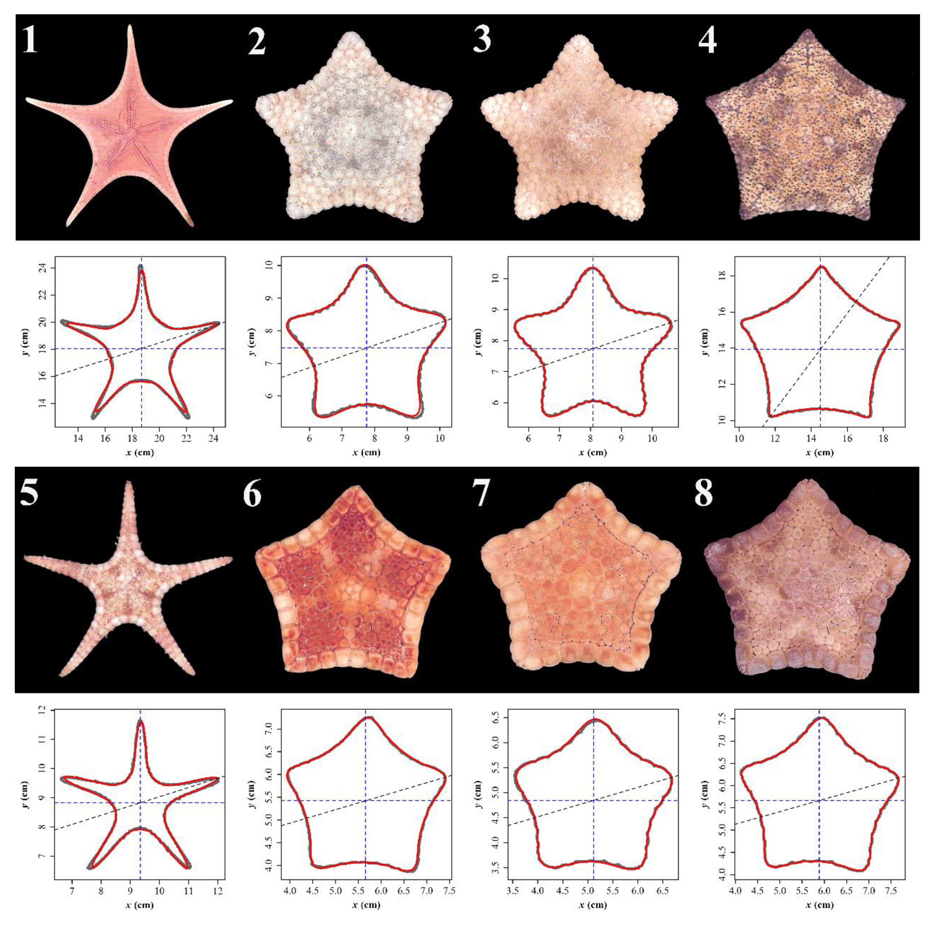
Figure 2 shows the original images and the fitted results for the edge data of eight starfish using GGE, and Figure 3 shows the fitted functional relationships (i.e., link functions) between r and re of the eight starfish on a log–log plot. Figure 4 exhibits the fitted leaf shapes and corresponding link functions for the four leaves on a log–log plot. Table A2 in Appendix A tabulates the estimated parameters and indicators of goodness of fit.
From Table A2, we can see most of the fitted results are satisfactory, with 10 out of the 12 RMSE values smaller than 0.1. Samples 1, 5 and 12 have RMSE values > 0.10. Overall, the adjusted RMSE values are significantly correlated with the RMSE values (r = 0.93, where r denotes the correlation coefficient; p < 0.05) for the 12 samples. This means that the influence of the object’s size on the goodness of fit (represented by RMSE) is not large for most of the investigated samples. For samples 2 and 4, the RMSE values are approximate (0.0510 vs. 0.0562); however, the adjusted RMSE of sample 2 is larger than that of sample 4 (0.0249 vs. 0.0151) because of the influence of size difference (13.16 cm2 vs. 43.22 cm2). It proves that the adjusted RMSE is more valid than RMSE in comparing the goodness of fit when there is a large difference in size between any two objects.
4. Discussion
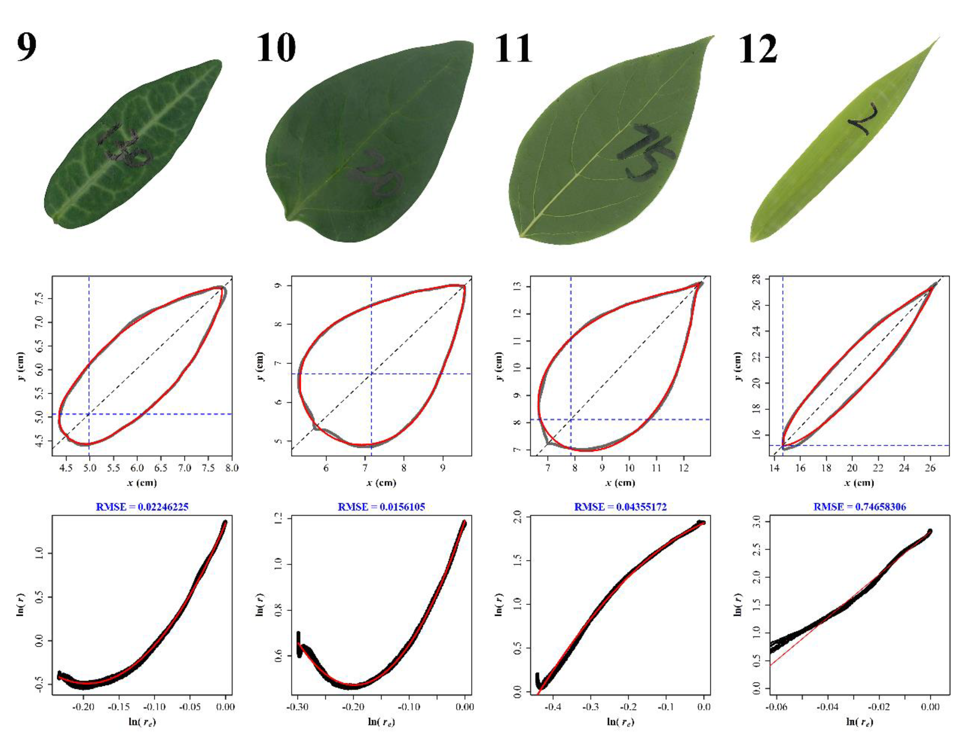
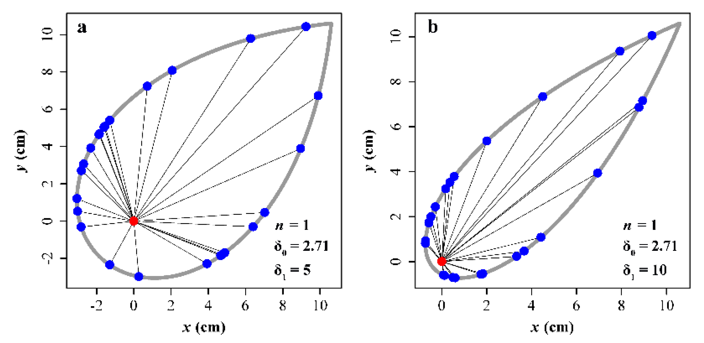
In Table A1, samples 1, 5 and 12 have larger RMSE values (>0.10) than the others. For the first two samples, the two starfish have relatively longer arms than the other 7 starfish. can be considered to be an “average absolute deviation”, that is, an average difference, ignoring sign, between the observed and predicted radii. According to Taylor’s power law, there is a power-law relationship with an exponent >0 (usually falling within a range of 1 to 3) between the variance and mean of a non-negative random variable [17,18]. In other words, the variance (and its square root) is an increasing function of the mean. Similarly, the RMSE of radii is positively related to the size of the object and the extent of variation in polar radii. The bigger the object is or the larger the extent of variation in polar radii is, the larger is its RMSE value. That is why samples 1 and 5 have large RMSE values. However, for sample 12, the main reason for its large RMSE value is as a result of the fitting approach. We minimized RSS as the target function of convergence. For the generalized Gielis curve that we used to depict the blade with a power-law function, the polar point was very close to the leaf base (i.e., the connection point of the blade and the petiole) if the leaf is narrow [10,11]; [also see Figure 5 below]. The ratio of leaf width to length has a big effect on the goodness of fit. A broad leaf shape ensures that the radii for the data points on the edge of a leaf close to the polar point are not too small, which enhances the goodness of fit when RSS is minimized as the target function. However, a narrow leaf shape gives rise to many small radii for the data points on the edge of the leaf near to the polar point, and that results in a large deviation between the actual and predicted radii (Figure 5). There are many data points that are far away from the polar point for a narrow leaf shape. Minimizing RSS will tend to reduce the deviations for these data points because the radii are larger than those of the data points close to the polar point. Unfortunately, most bamboo leaves are narrow [19]. Thus, the minimization of RSS has resulted in a large deviation for the data points close to the polar point. That is why sample 12 fits the data worse than the other samples. The quadratic function given by Equation (13) with δ2 ≠ 0 did not improve the goodness of fit.
For leaves which are flat, the 2D representations are of immediate value to quantify shape and area. For starfish, the 2D representations can serve as one of the two sections to build a 3D starfish. Whether the proposed two functions (i.e., the hyperbolic and quadratic equations) can apply to more shapes is still unknown, meriting further investigation. We believe that other forms of link functions can be found for shapes that cannot be adequately fitted by Equations (12) and (13).
5. Conclusions
In the present study, we propose a generalized Gielis equation (GGE) by introducing a link function for the polar radius of the elementary Gielis equation (EGE). The original Gielis equation (OGE) can then be regarded as a special case of GGE with a power-law link function between the polar radius of EGE and that of GGE. Although OGE can produce a lot of shapes, the power-law link function has limited validity for describing shapes such as the planar projection of starfish. In that case, we put forward two candidate link functions (a log-hyperbolic function and a log-quadratic function) to make OGE applicable to these shapes. We found that these two functions describe the shapes of the investigated starfish and leaves well, showing that in nature, not all ontogenetic radial growth follows the power-law relationship.
Supplementary Materials
The following are available online at https://0-www-mdpi-com.brum.beds.ac.uk/2073-8994/12/4/645/s1, Appendix S1: R script for extracting the planar coordinates of an image, Appendix S2: R script for fitting the edge data using the generalized Gielis equation.
Author Contributions
P.S. and J.G. conceived and designed the experiment together; P.S. and D.A.R. analyzed the data; P.S., D.A.R. and J.G. wrote the manuscript. All authors have read and agreed to the published version of the manuscript.
Funding
This research was funded by the Jiangsu Government Scholarship for Overseas Studies (grant number: JS-2018-038).
Conflicts of Interest
The authors declare no conflict of interest.
Appendix A
There are two tables for tabulating the sample collection information and the fitted results using the generalized Gielis equation, respectively.

Table A1.
Sample collection information.
| Sample Code | Scientific Name | Family | Locality | Sampling Time |
|---|---|---|---|---|
| 1 | Anthenoides tenuis Liao & A.M. Clark | Goniasteridae | Philippines, Siquijor | 2019 |
| 2 | Culcita schmideliana Bruzelius | Oreasteridae | Philippines, Bohol. Cabulan Island | 2018 |
| 3 | Culcita schmideliana Bruzelius | Oreasteridae | Philippines, Bohol. Cabulan Island | 2018 |
| 4 | Culcita schmideliana Bruzelius | Oreasteridae | Philippines, Bohol. Cabulan Island | 2018 |
| 5 | Stellaster equestris Bruzelius | Goniasteridae | Philippines, Surigao | 2018 |
| 6 | Tosia australis Gray | Goniasteridae | Edithburgh, Australia | 1980 |
| 7 | Tosia magnifica Müller & Troschel | Goniasteridae | Edithburgh, Australia | 1980 |
| 8 | Tosia magnifica Müller & Troschel | Goniasteridae | Edithburgh, Australia | 1980 |
| 9 | Trachelospermum jasminoides (Lindl.) Lem. | Apocynaceae | Nanjing, China | 2019 |
| 10 | Vinca major L. | Apocynaceae | Nanjing, China | 2018 |
| 11 | Chimonanthus praecox (L.) Link | Calycanthaceae | Nanjing, China | 2017 |
| 12 | Phyllostachys incarnata T.H. Wen | Poaceae | Nanjing, China | 2016 |
Table A2.
Estimated parameters and indicators for goodness of fit.
| Code | Sample Size | Area (cm2) | RSS | RMSE | RMSEadj | |||||||
| 1 | 18.67 | 18.05 | 1.56 | 2006.90 | 1.1362 | 0.0599 | 0.8742 | 2488 | 32.00 | 235.22 | 0.3075 | 0.0963 |
| 2 | 7.75 | 7.47 | 2.85 | 8.39 | 2.0738 | 4.2943 | 0.4556 | 1482 | 13.16 | 3.8561 | 0.0510 | 0.0249 |
| 3 | 8.08 | 7.74 | 1.58 | 4.83 | 1.5802 | 3.7025 | 0.3311 | 1617 | 13.52 | 1.2516 | 0.0278 | 0.0134 |
| 4 | 14.51 | 13.94 | 0.30 | 139.04 | 2.8784 | 0.6546 | 1.1619 | 2684 | 43.22 | 8.4710 | 0.0562 | 0.0151 |
| 5 | 9.34 | 8.83 | 0.31 | 543.36 | 0.8644 | 0.1151 | −0.1390 | 2282 | 6.09 | 34.53 | 0.1230 | 0.0883 |
| 6 | 5.66 | 5.42 | 0.29 | 7.73 | 2.7866 | 6.8694 | 0.2415 | 1526 | 7.37 | 0.4804 | 0.0177 | 0.0116 |
| 7 | 5.11 | 4.85 | 0.29 | 4.28 | 2.3100 | 5.4630 | 0.0503 | 1263 | 6.07 | 0.5415 | 0.0207 | 0.0149 |
| 8 | 5.88 | 5.66 | 2.79 | 5.95 | 2.6437 | 7.5884 | 0.2371 | 1267 | 7.58 | 0.3502 | 0.0166 | 0.0107 |
| Code | Sample Size | Area (cm2) | RSS | RMSE | RMSEadj | |||||||
| 9 | 4.98 | 5.06 | 0.76 | 1.32 | 1.3485 | 18.8344 | 48.2690 | 1653 | 5.40 | 2.7591 | 0.0409 | 0.0312 |
| 10 | 7.16 | 6.73 | 0.76 | 1.14 | 1.1925 | 7.2615 | 18.3014 | 1379 | 11.65 | 1.1927 | 0.0294 | 0.0153 |
| 11 | 7.84 | 8.12 | 0.81 | 0.73 | 1.9303 | 1.9169 | −5.7404 | 1985 | 22.25 | 8.9448 | 0.0671 | 0.0252 |
| 12 | 14.67 | 15.22 | 0.81 | 1.23 | 2.8179 | 38.5217 | 0 | 2476 | 33.22 | 350.16 | 0.3761 | 0.1156 |
In this table, Code represents the sample code (see Table A1 for details); (, ) represents the estimated planar coordinates of the polar point; represents the estimated angle by which the horizontal line (i.e., the original x-axis) of the generalized Gielis curve was rotated; , , , , and are estimated parameters in Equations (12) and (13); Sample size represents the number of data points on the edge of an image; Area represents the scanned (actual) area of a starfish or leaf image; RSS is the residual sum of squares; RMSE is the root-mean-square error; RMSEadj is the adjusted root-mean-square error.
References
- Gielis, J. A general geometric transformation that unifies a wide range of natural and abstract shapes. Am. J. Bot. 2003, 90, 333–338. [Google Scholar] [CrossRef] [PubMed]
- Gielis, J. The Geometrical Beauty of Plants; Atlantis Press: Paris, France, 2017. [Google Scholar]
- Shi, P.J.; Huang, J.G.; Hui, C.; Grissino-Mayer, H.D.; Tardif, J.; Zhai, L.H.; Wang, F.S.; Li, B.L. Capturing spiral radial growth of conifers using the superellipse to model tree-ring geometric shape. Front. Plant Sci. 2015, 6, 856. [Google Scholar] [CrossRef] [PubMed] [Green Version]
- Wei, Q.; Jiao, C.; Guo, L.; Ding, Y.L.; Cao, J.J.; Feng, J.Y.; Dong, X.B.; Mao, L.Y.; Sun, H.H.; Yu, F.; et al. Exploring key cellular processes and candidate genes regulating the primary thickening growth of Moso underground shoots. New Phyotol. 2017, 214, 81–96. [Google Scholar] [CrossRef] [PubMed]
- Guo, L.; Sun, X.P.; Li, Z.R.; Wang, Y.J.; Fei, Z.J.; Chen, J.; Feng, J.Y.; Cui, D.F.; Feng, X.Y.; Ding, Y.L.; et al. Morphological dissection and cellular and transcriptome characterizations of bamboo pith cavity formation reveal a pivotal role of genes related to programmed cell death. Plant Biotechnol. J. 2019, 17, 982–997. [Google Scholar] [CrossRef] [PubMed]
- Tian, F.; Wang, Y.J.; Sandhu, H.S.; Gielis, J.; Shi, P.J. Comparison of seed morphology of two ginkgo cultivars. J. Forest Res. 2018. [Google Scholar] [CrossRef]
- Shi, P.J.; Liu, M.D.; Yu, X.J.; Gielis, J.; Ratkowsky, D.A. Proportional relationship between leaf area and the product of leaf length and width of four types of special leaf shapes. Forests 2019, 10, 178. [Google Scholar] [CrossRef] [Green Version]
- Caratelli, D.; Gielis, J.; Tavkhelidze, I.; Ricci, P.E. Fourier-Hankel solution of the Robin problem for the Helmholtz equation in supershaped annular domains. Bound. Value Probl. 2013, 2013, 253. [Google Scholar] [CrossRef] [Green Version]
- Matsuura, M. Gielis’ superformula and regular polygons. J. Geom. 2015, 106, 383–403. [Google Scholar] [CrossRef]
- Shi, P.J.; Xu, Q.; Sandhu, H.S.; Gielis, J.; Ding, Y.L.; Li, H.R.; Dong, X.B. Comparison of dwarf bamboos (Indocalamus sp.) leaf parameters to determine relationship between spatial density of plants and total leaf area per plant. Ecol. Evol. 2015, 5, 4578–4589. [Google Scholar] [CrossRef] [PubMed]
- Lin, S.Y.; Zhang, L.; Reddy, G.V.P.; Hui, C.; Gielis, J.; Ding, Y.L.; Shi, P.J. A geometrical model for testing bilateral symmetry of bamboo leaf with a simplified Gielis equation. Ecol. Evol. 2016, 6, 6798–6806. [Google Scholar] [CrossRef] [PubMed]
- Koiso, M.; Palmer, B. Rolling construction for anisotropic Delaunay surfaces. Pac. J. Math. 2008, 234, 345–378. [Google Scholar]
- Wei, H.L.; Li, X.M.; Huang, H. Leaf shape simulation of castor bean and its application in nondestructive leaf area estimation. Int. J. Agric. Biol. Eng. 2019, 12, 135–140. [Google Scholar]
- Ratkowsky, D.A. Nonlinear Regression Modeling: A Unified Practical Approach; Marcel Dekker: New York, NY, USA, 1983. [Google Scholar]
- Spiess, A.-N.; Neumeyer, N. An evaluation of R squared as an inadequate measure for nonlinear models in pharmacological and biochemical research: A Monte Carlo approach. BMC Pharmacol. 2010, 10, 6. [Google Scholar] [CrossRef] [PubMed] [Green Version]
- R Core Team. R: A Language and Environment for Statistical Computing; R Foundation for Statistical Computing: Vienna, Austria, 2019; Available online: https://www.R-project.org/ (accessed on 1 January 2020).
- Giometto, A.; Formentin, M.; Rinaldo, A.; Cohen, J.E.; Maritan, A. Sample and population exponents of generalized Taylor’s law. Proc. Natl. Acad. Sci. USA 2015, 112, 7755–7760. [Google Scholar] [CrossRef] [PubMed] [Green Version]
- Shi, P.J.; Ratkowsky, D.A.; Wang, N.T.; Li, Y.; Reddy, G.V.P.; Zhao, L.; Li, B.L. Comparison of five methods for parameter estimation under Taylor’s power law. Ecol. Compl. 2017, 32, 121–130. [Google Scholar] [CrossRef]
- Lin, S.Y.; Niklas, K.J.; Wan, Y.W.; Hölscher, D.; Hui, C.; Ding, Y.L.; Shi, P.J. Leaf shape influences the scaling of leaf dry mass vs. area: A test case using bamboos. Ann. Forest Sci. 2020, 77, 11. [Google Scholar] [CrossRef] [Green Version]
Figure 1.
A simulation example of the generalized Gielis curve. In panel (a), the red curve represents the elementary Gielis curve, and the black curve represents the generalized Gielis curve (m = 5, k = 1, n2 = n3 = 5, a = 2.0, b = 1.5 and c = 0.2); in panel (b), the red curve represents the link function between r and re according to Equation (10); in panel (c), the red curve represents the link function on the log–log plot according to Equation (12).

Figure 2.
Original images of eight starfish (codes 1−8 in Table A1) and fitted generalized Gielis curves. The number in the upper left corner for each black background image panel represents its sample code. The panel below each black background image panel shows the scanned edge (represented by a gray curve) and the fitted edge using GGE (represented by a red curve). The intersection between the blue vertical and horizontal dashed lines represents the polar point; the black inclined dashed line represents the previously used horizontal line of a standard GGE without an angle transformation.

Figure 3.
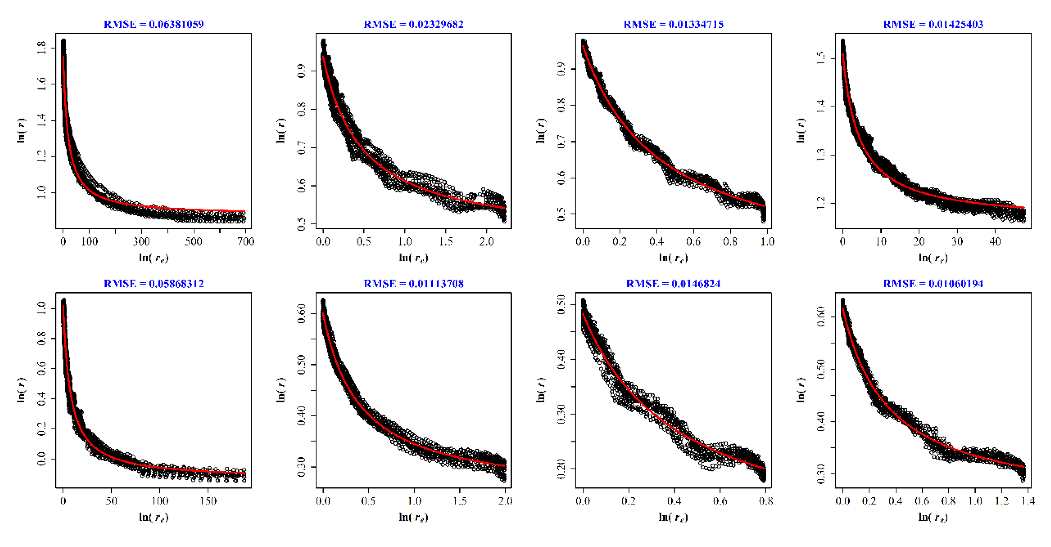
The scatter plots of ln(r) vs. ln(re) and the fitted link functions for each of the eight starfish. In each panel, the small open circles represent the actual values, and the red curve represents the fitted link function based on Equation (12). RMSE values shown here were calculated based on the log-transformed data, while RMSE values in Table A1 were based on the untransformed data of r vs. re.
Figure 3.
The scatter plots of ln(r) vs. ln(re) and the fitted link functions for each of the eight starfish. In each panel, the small open circles represent the actual values, and the red curve represents the fitted link function based on Equation (12). RMSE values shown here were calculated based on the log-transformed data, while RMSE values in Table A1 were based on the untransformed data of r vs. re.

Figure 4.
Original images, scanned and predicted leaf edges, and fitted link functions on a log–log plot for four plant species (codes 9–12 in Table A1). The number in the upper left corner for each green image panel represents its sample code. The panel below each green image panel shows the scanned edge (represented by a gray curve) and the fitted edge using GGE (represented by a red curve). In each panel in the bottom row, the small open circles represent the actual values of ln(r) vs. ln(re), and the red curve represents the fitted link function based on Equation (13).

Figure 5.
Illustration for the comparison between a broad blade (a) and a narrow blade (b). In each panel, the red point represents the polar point; the blue points represent the data points on the edge of the blade; the gray curve represents the blade edge; the segments between the polar point and the data points on the edge represent radii. Each leaf shape was generated by GGE with a power-law relationship (which is equation [13] when δ2 = 0). The horizontal axis of the generalized Gielis curve is rotated counterclockwise by π/4 to conveniently show the image. Here, when δ1 decreases towards 0, the curve approximates a circle with radius exp(δ0) and the polar point becomes the center of this circle at the point (0, 0). In contrast, when δ1 increases towards a large value, the curve approximates a line segment with length exp(δ0) and the polar point approaches the left endpoint of the segment.

© 2020 by the authors. Licensee MDPI, Basel, Switzerland. This article is an open access article distributed under the terms and conditions of the Creative Commons Attribution (CC BY) license (http://creativecommons.org/licenses/by/4.0/).
Share and Cite
MDPI and ACS Style
Shi, P.; Ratkowsky, D.A.; Gielis, J. The Generalized Gielis Geometric Equation and Its Application. Symmetry 2020, 12, 645. https://0-doi-org.brum.beds.ac.uk/10.3390/sym12040645
AMA Style
Shi P, Ratkowsky DA, Gielis J. The Generalized Gielis Geometric Equation and Its Application. Symmetry. 2020; 12(4):645. https://0-doi-org.brum.beds.ac.uk/10.3390/sym12040645
Chicago/Turabian StyleShi, Peijian, David A. Ratkowsky, and Johan Gielis. 2020. "The Generalized Gielis Geometric Equation and Its Application" Symmetry 12, no. 4: 645. https://0-doi-org.brum.beds.ac.uk/10.3390/sym12040645
Note that from the first issue of 2016, this journal uses article numbers instead of page numbers. See further details here.