Trajectory Planning for Mechanical Systems Based on Time-Reversal Symmetry

Abstract

The generation of feasible trajectories poses an eminent task in the field of control design in mechanical systems. The paper demonstrates innovative approach in trajectory planning for mechanical systems via time-reversal symmetry. It also presents two case studies: mass-spring-damper and inverted pendulum on the cart. As real systems break the time-reversal symmetry, the authors of this work propose a unique method in order to overcome this drawback. It computes a feed-forward reference control signal and state trajectories. The proposed solution enables compensation for the effects of couplings, which break the time-symmetry by a special proposed measure. The method suppresses the overall open-loop accumulated error and produces high-quality favorable control and state trajectories. Furthermore, the existence of the designed control signal and state trajectories is guaranteed if the equations of the motion have a solution in the direct flow of time.

1. Introduction

The general framework of this paper is a trajectory planning problem. It is also referred to as a finite-time transition problem because the main area of interest is a computation of a feed-forward open-loop control signal capable of performing transition between equilibrium points. In mathematical nomenclature, solution of such problem corresponds to a two-point boundary value problem (TPBvP).

For a general Hamiltonian dynamical system, a TPBvP problem can be solved using different iterative techniques. The first set of methods, called shooting methods, bases on choosing values for all of the dependent variables at one boundary, consistent with boundary conditions [1,2,3]. Then, iteratively system’s equations are integrated, and the initial guess is modified to minimize discrepancies between boundaries. The second set of techniques base on relaxation methods [4], where the differential equations are replaced by finite-difference equations on a mesh of points that covers the range of the integration. During iterative relaxation, the values on the mesh are adjusted to minimize differences with the finite-difference equations and with the boundary conditions. The main drawback of the above-mentioned methods is excessive computation burden while modeling non-linear systems. Therefore, the new approaches are studied extensively, e.g., generating functions technique [5].

This paper introduces a new method of finding a feed-forward open-loop control signal with the use of time-reversal symmetry applied for mechanical systems under the presence of damping or friction which, together with the possibility of extension of this approach for other nonlinear dynamic systems. The method proposed of the authors of this work is a novel approach to TPBvP problem and has not been applied before.

The paper is organized in the following way: in Section 2, the motivational case study is presented, where the mass-spring-damper model is described, with its trajectory planning based on time-reversal symmetry. Then the primary case study, i.e., swing-up of the inverted pendulum on the cart is given, and the reversibility of this model is explained. Then the methodology of the time-reversal symmetry applied to the inverted pendulum model, allowing to deal with friction presence is proposed. In Section 3 the results of the numerical trajectory planning for the swing-up of the inverted pendulum are gathered. In Section 4 the methodology and obtained research results are discussed. Finally, concluding remarks are given in Section 5.

Background to the Study

Time-reversal symmetry is a significant feature of a dynamic system. A system is time-reversal symmetric if it shows an identical behavior independent of the flow of time. A simple explanation is given in [6]: watching a movie, which shows a movement of an ideal pendulum, an observer is unable to determine if the movie plays in forward or in backward direction. However, considering a more realistic physical situation of a swinging pendulum under the presence of a friction, there is a difference between a forward and a reverse film of this pendulum. The original film shows the swinging pendulum losing its amplitude until it reaches a steady state corresponding to a lower stable position. The reversed film shows the pendulum whose amplitude keeps increasing in time. The latter film clearly clashes with physics as it does not follow the natural laws of motion. It can be said that the presence of a friction breaks the time-reversal symmetry of the ideal friction-less pendulum. The ideal pendulum is a non-existing object, whose description can be found in numerous physics books and is not affected by frictional forces, what enables it to oscillate with an isochronous period. It has been subject of numerous studies for decades [7,8,9]. In field of dynamic systems, the first time the time symmetry was used dates back to 1915 when the restricted three body problem was analyzed in [10]. Later on, in the 1960s, the topic of time-symmetry was studied by mathematicians [11,12,13,14,15] followed by others one decade later [16,17]. However the most known problems relate to the fields of thermodynamics and quantum mechanics, see [18,19,20]. The first motivation for this paper was inspired with the following paper: [21], and the most important symmetry-related issues with inverted pendulum models are discussed in [22,23]. However, the most comprehensive paper on the given topic is [6], which discusses time-reversal symmetry in physics generally, then for dynamic systems, tackling various aspects of reversible dynamics and also the extensive study carried out [24] explains relations between time-reversal systems, differential equations of the systems, conservative and dissipative behavior and chaos. The objective of the paper can be formulated as follows. There exists a given mechanical system—an inverted pendulum on the cart moving on linear guide rails, which was in detail described in inter alia [25]. For such a system it is possible to compute a feed-forward reference control based on time-reversal symmetry, which generates feasible trajectories. The calculation of the proposed control signal uses compensation for the couplings, which break the time-symmetry.

2. Materials and Methods

This paper focuses on two case studies, which fall under the field of classical mechanics systems (mass-spring-damper, inverted pendulum) as described together with other similar problems in [26]. The process of trajectory generation is documented in this paper through a case study of a single inverted pendulum on the cart moving on linear guide rails, starting with an introductory example of a mass-spring-damper model. Presence of friction or damping is the main reason for the breaking of the time-reversal symmetry in mechanical systems and this problem was deeply studied in [27].

2.1. Motivational Case Study: Mass-Spring-Damper Model

This part of the paper presents the main idea of the proposed solution’s application based on a basic example of a linear system. It clearly shows how and why the time-reversal symmetry is broken and shows the necessary steps of computation of a feed-forward open-loop control signal while considering a damping presence. The mass-spring-damper model is described by the following equation.

$$m·\ddot{y}(t)+b·\dot{y}(t)+k·y(t)=F(t).$$

(1)

where $F(t)$ [N] stands for an external force representing input to the dynamic system; m [kg] is a mass; b [N·s·m⁻¹] is a damping coefficient; k [N·m⁻¹] is a spring stiffness; $y(t)$ is the output of the dynamic system (position of the mass), $\dot{y}(t)$, $\ddot{y}(t)$ are first and second derivative of $y(t)$ respectively (velocity and acceleration). Assuming no external force, the mass-spring-damper model can be described by the following 2^nd order ordinary differential equation

$$m·\ddot{y}(t)+b·\dot{y}(t)+k·y(t)=0.$$

(2)

Reversing the flow of time by introducing a new variable $\vartheta =T-t$ representing the reverse time, the reversal movement can be described by

$$m·\ddot{y}(\vartheta )+b·\dot{y}(\vartheta )+k·y(\vartheta )=0.$$

(3)

Then a time-reversal motion $y_i(t)=y(\vartheta )$, $t\in [0,T]$ can be introduced. Because ${\dot{y}}_i(t)=-\dot{y}(\vartheta )$ and ${\ddot{y}}_i(t)=\ddot{y}(\vartheta )$, then the following applies

$$m·{\ddot{y}}_i(t)-b·{\dot{y}}_i(t)+k·y_i(t)=0.$$

(4)

Thus $y_i(t)$ can be a solution of Equation (2) if and only if $b=0$ and violates the symmetry principle for other values. In other words, time-reversal symmetry is not valid for Equation (2) unless no damping is present.

2.1.1. State-Space Description of Mass-Spring-Damper Model

For the demonstration purposes the capabilities of the proposed method for planning the trajectory for the mass-spring-damper model, the following state-space description of Equation (2) will be used:

$$\left\{\begin{array}{c}{\dot{x}}_1(t)=x_2(t)\hfill \\ {\dot{x}}_2(t)=\frac{1}{m}·u(t)-\frac{b}{m}·x_2(t)-\frac{k}{m}·x_1(t)\hfill \end{array}\right.$$

(5)

where $x_1(t)$ [m]—mass position; $x_2(t)$ [m·s⁻¹]—velocity; $u(t)$ [N]—force.

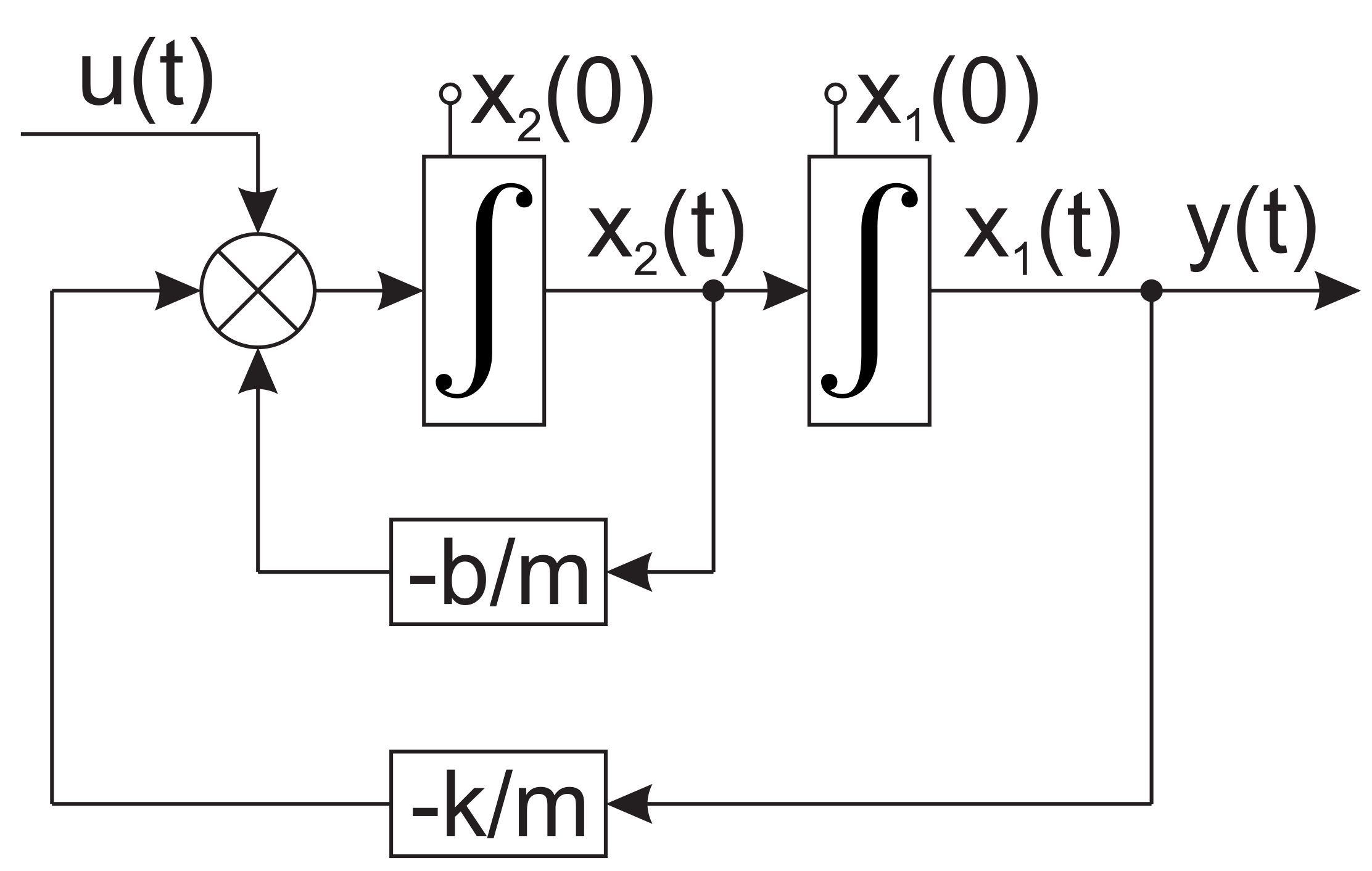
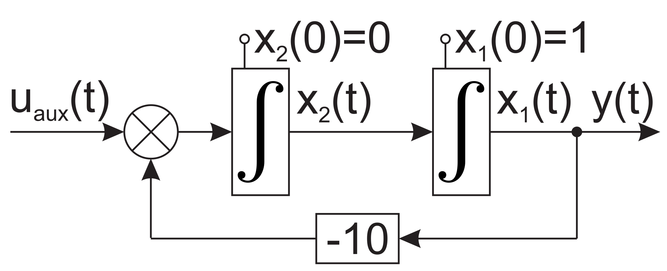
The mass position is chosen as the output, $y(t)\equiv x_1(t)$. The state-space scheme of the model is then expressed by Figure 1. The following values of the parameters are used throughout this initial case study: $m=1$, $b=0.5$, $k=10$, $x_2(0)=0$, $x_1(0)=0$, $T=1$. The problem is defined as trajectory planning so that the system reaches predefined final state $x_2(T)=0$, $x_1(T)=1$. Note that the only one state $x_1(t)\equiv y(t)$ will be considered throughout further explanation.

2.1.2. Trajectory Planning for Mass-Spring-Damper Model

Computation of a feed-forward open-loop control signal can be demonstrated in a simulation experiment according to the design procedure described in the following consecutive steps. This design procedure can be used in general for any linear time-invariant (LTI) system. Extension to the nonlinear system via case study is described in the next section of this paper.

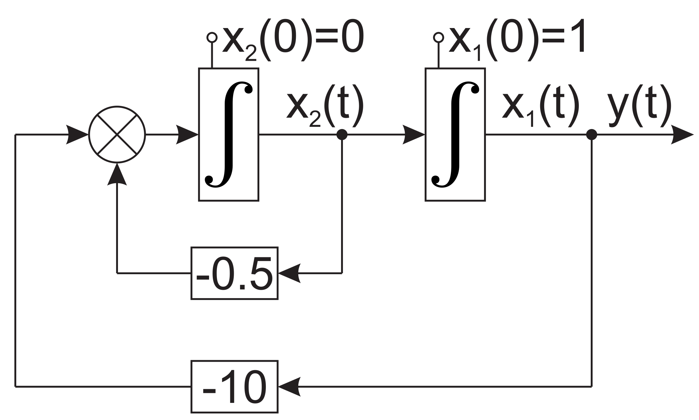
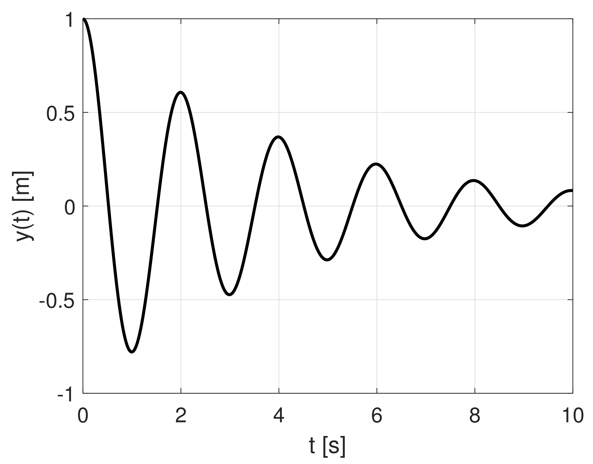
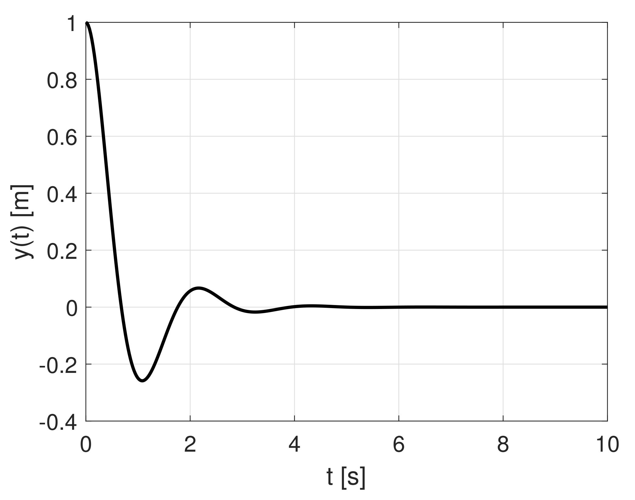
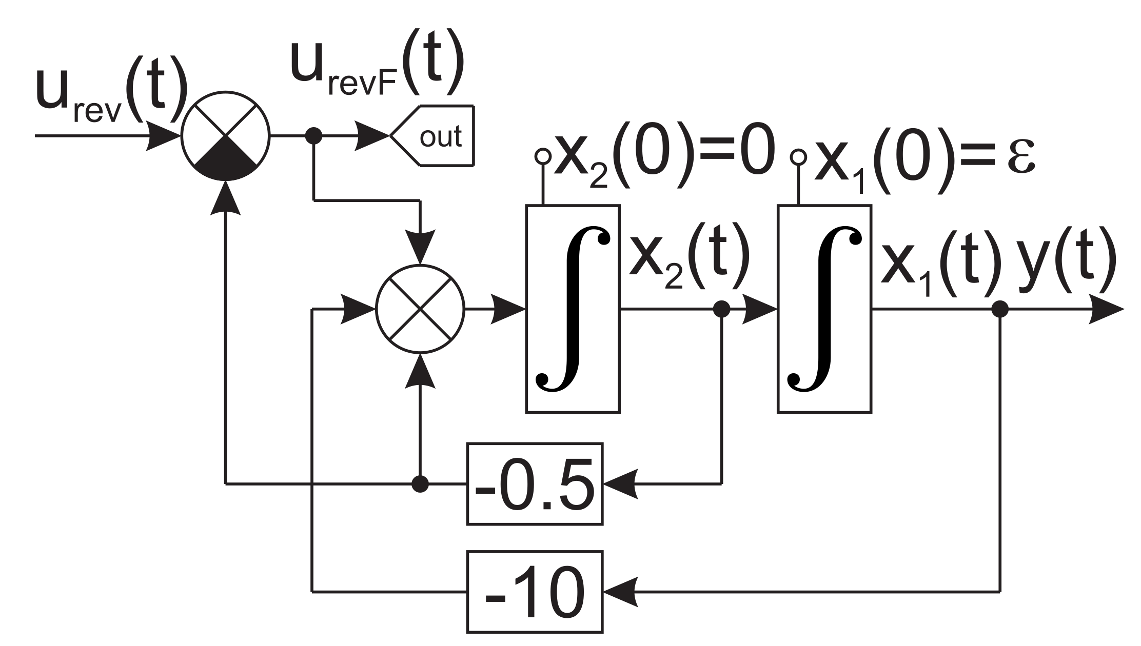
• Obtaining a response to initial conditions $x_2(0)$, $x_1(0)$ whose values correspond to the predefined final state $x_2(T)=0$, $x_1(T)=1$ are supposed to reach at time $t=T$ by application of so far unknown control signal $u(t)$ brought to the input of the system according to Figure 2. Note that the input $u(t)$ is absent at the moment. Resulting waveform is depicted in Figure 3.
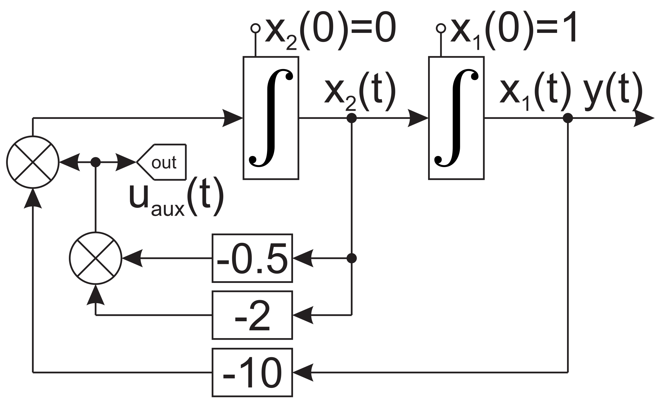
• As the output signal shown in Figure 3 is too oscillatory to represent a good candidate for a trajectory, the scheme depicted in Figure 2 is modified by adding an artificial damping to the system and stores the signal referred to as $u_{aux}(t)$ is provided, where $u_{aux}(t)=-2.5·x_2(t)$. The value of the damping parameter was adjusted to keep the stability of the system and obtain the sufficient system’s response in time and frequency domains. This modified scheme is depicted in Figure 4 and its simulation leads to the waveform shown in Figure 5 which is now considered as an appropriate candidate for a state trajectory.
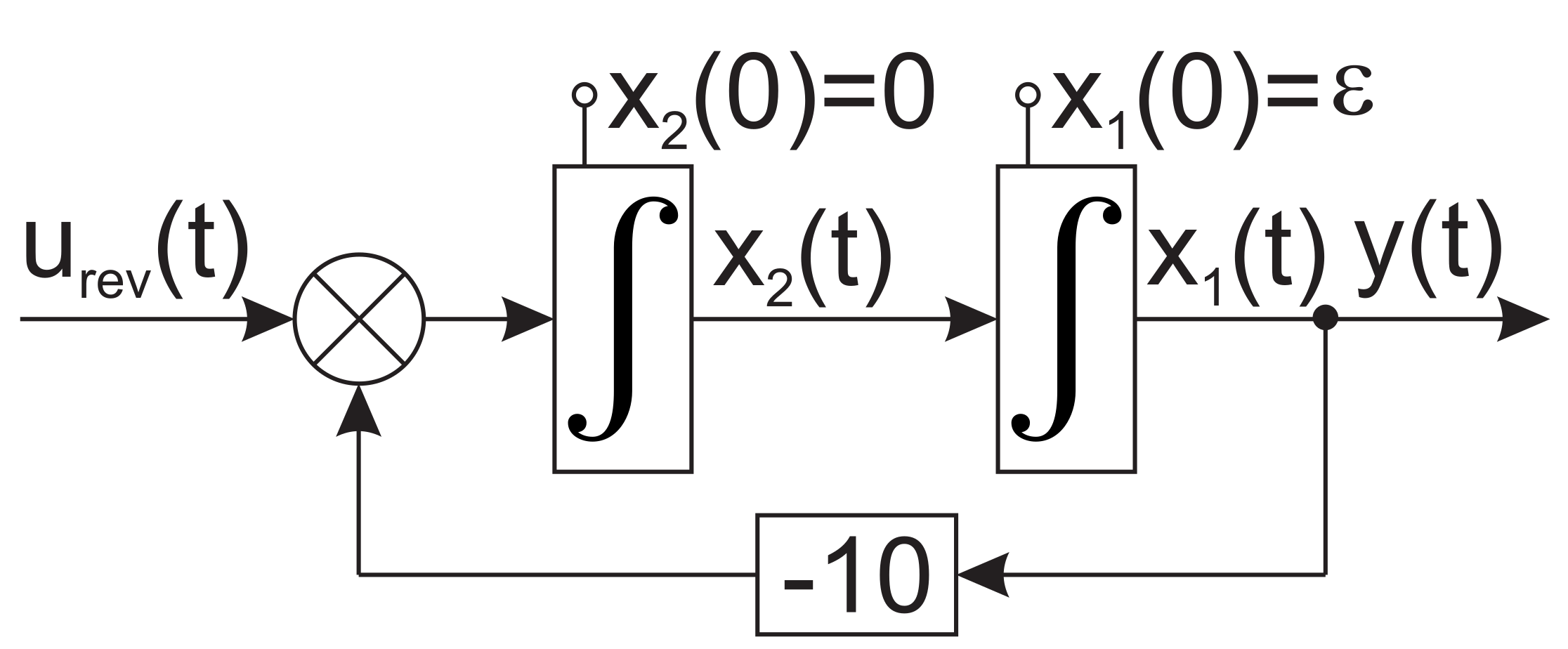
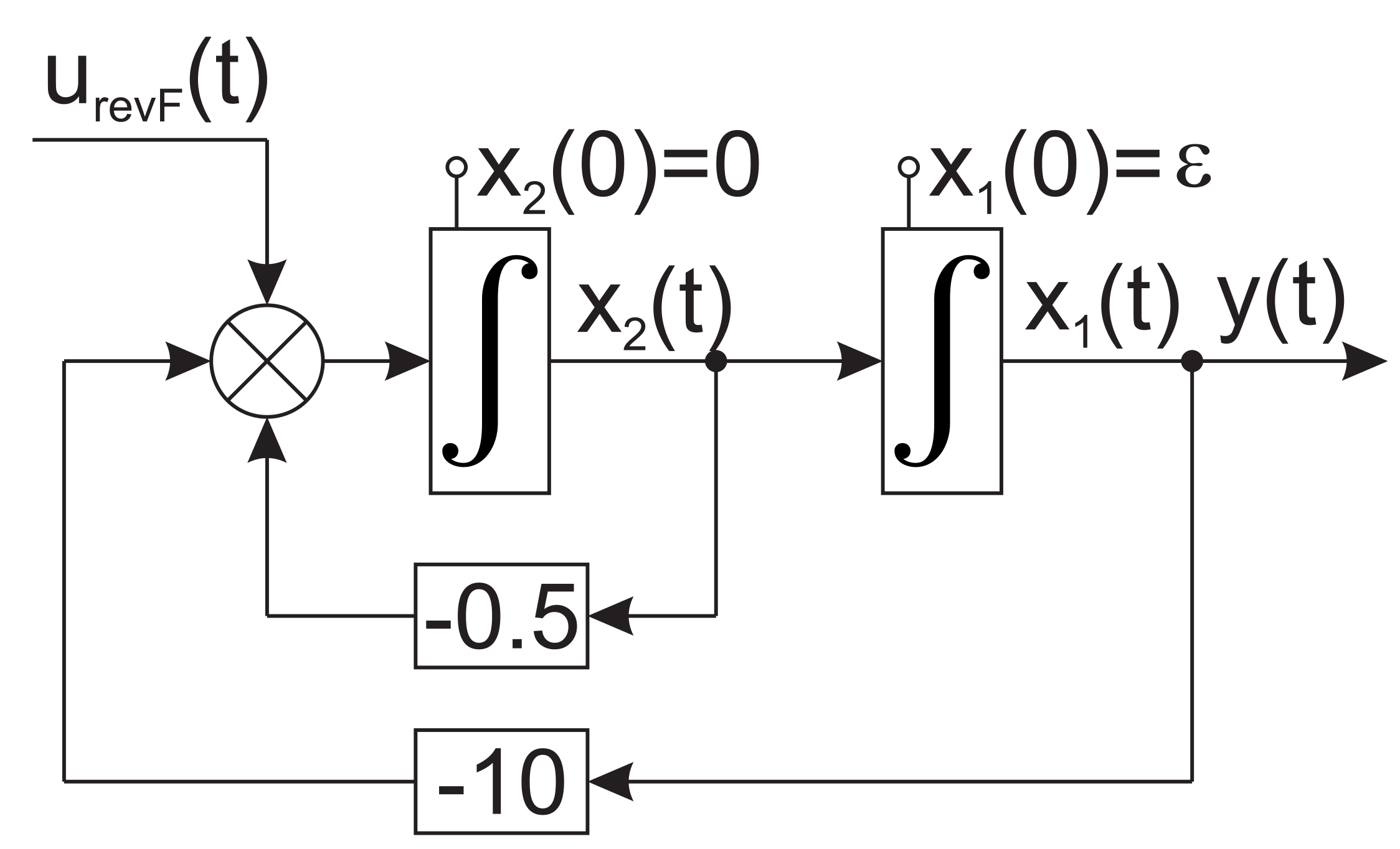
• The compensating damping is illustrated with the Figure 4 through an output drawn from $x_2(t)$ to be stored in $u_{aux}(t)$. This system is then simplified as presented with Figure 6 and continues to maintain time reversal symmetry. The simulation result from systems described in Figure 4 and Figure 6 give out identical waveform as shown in Figure 5.
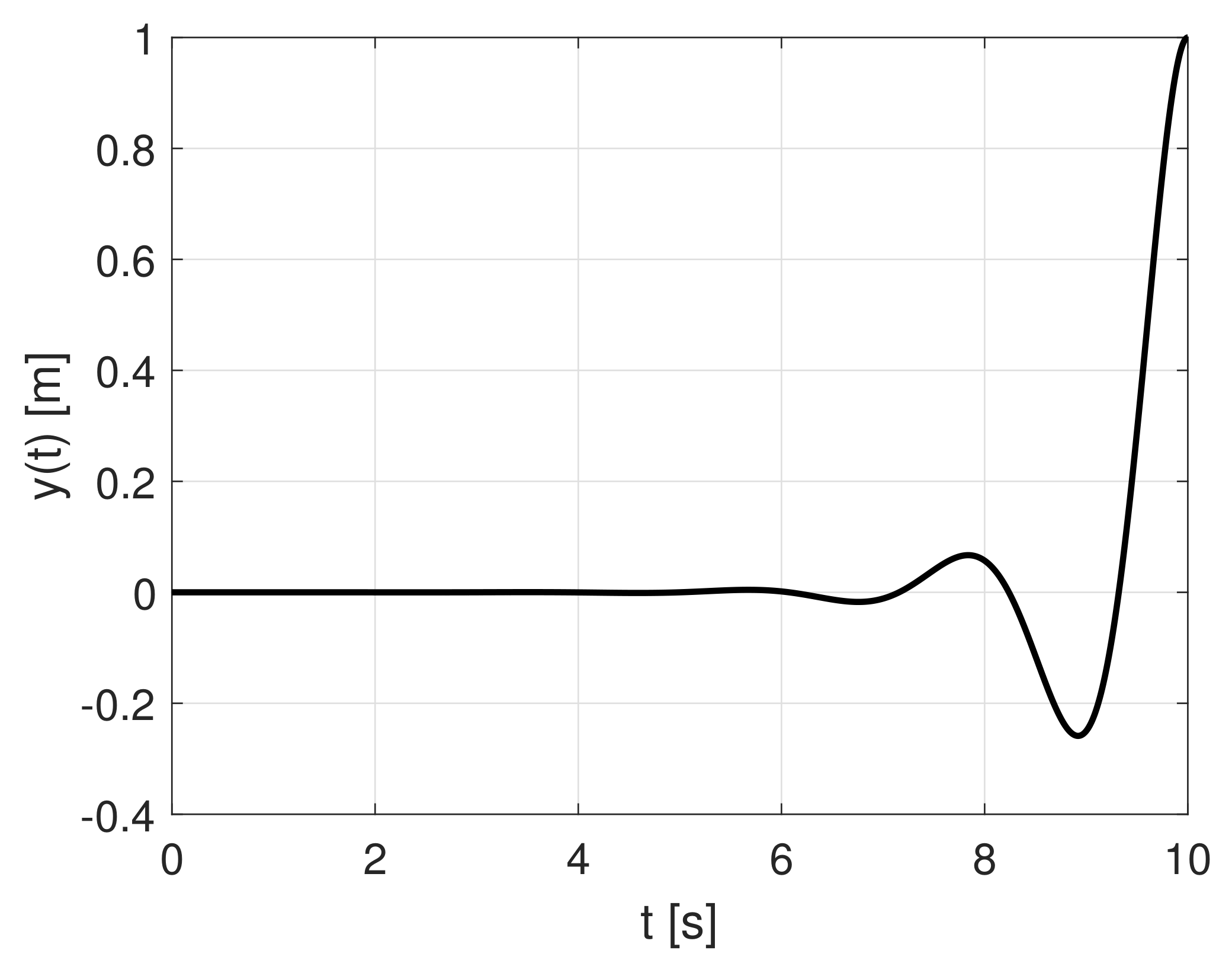
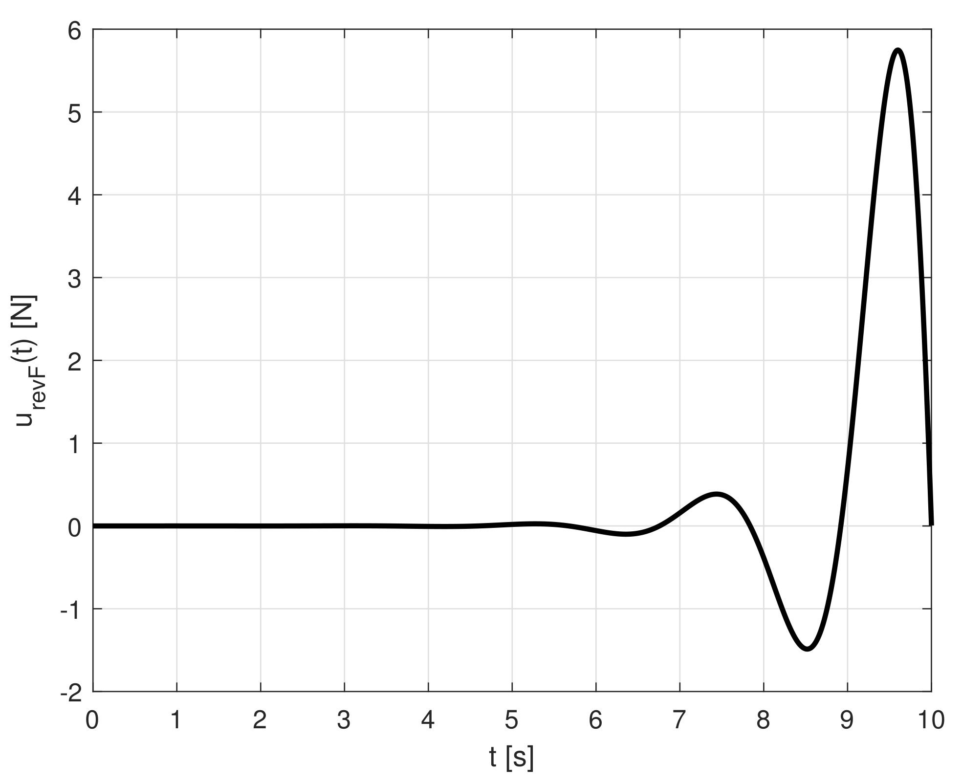
• Reversing the time flow of the control signal $u_{aux}(t)$ depicted in Figure 6 in time presented in Figure 7 into $u_{rev}(t)$ using the relation $u_{rev}(t)=u_{aux}(\vartheta )=u_{aux}(T-t)$. The initial conditions applied in Figure 7 will correspond to the final values reached in previous phase at the time $t=T$. Supposing adequate time range, in this case the values will be very close to zero, $x_2(0)=0$, $x_1(0)=\epsilon \approx 0$, respectively. Resulting waveform is depicted in Figure 8.
• Going back to the original model described in Figure 1. The effect of damping will be eliminated by subtracting the damping term from control signal $u_{rev}(t)$ which results in a control signal $u_{revF}(t)$ which is stored for further use as shown in Figure 9, where $u_{revF}(t)=u_{rev}(t)-0.5·x_2(t)$.
• Application of the control signal $u_{revF}(t)$ to the original system enables conclusion that the outputs from the simulation models in presented in Figure 7, Figure 8, Figure 10 and Figure 11 are identical. These outputs are equivalent to time-inversion of the output shown in Figure 5.

Reference control signal $u_{revF}(t)$ and corresponding reference output $y(t)\equiv x_1(t)$ have been obtained according to Figure 10 and shown in Figure 11 and Figure 12. This waveform fulfills predefined requirements defined at the beginning of the chapter. The reference control signal and reference state trajectories have been found and tested via simulation.

2.2. Primary Case Study: Swing-Up of the Inverted Pendulum on the Cart

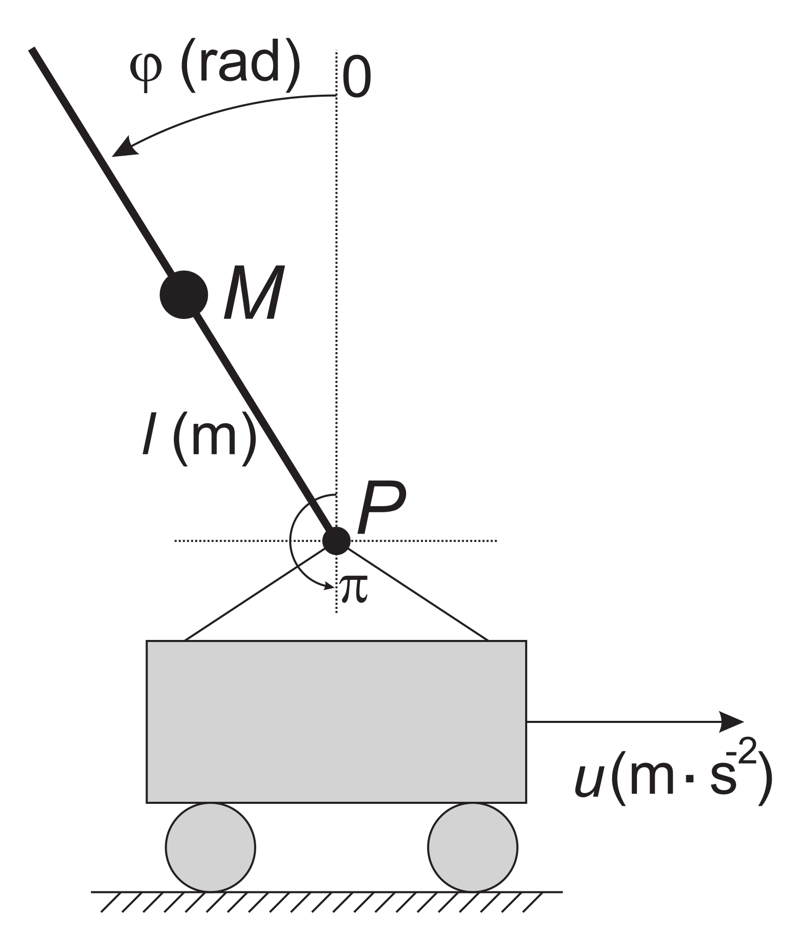
The scheme of the setup with the description of system variables and parameters used in this primary case study is given in Figure 13.

A nonlinear differential equation describing the movement of the inverted pendulum on the cart is adopted from [28]. The model of inverted pendulum in this paper assumes a homogeneous cylindrical rod of the length L [m] and thus $l=\left|MP\right|=\frac{1}{2}·L$ where $\left|MP\right|$ represents the distance from the pivot P to the center of the mass M. The model of an inverted pendulum on the cart is described by the differential equation as follows

$$\ddot{\phi }(t)-\frac{3}{4}·\frac{g}{l}·sin\phi (t)+b·\dot{\phi }(t)=\frac{3}{4}·\frac{1}{l}·u(t)·cos\phi (t),$$

(6)

where $\phi (t)$ [rad]—angular position of the rod with respect to vertical axis; $u(t)$ [m·s⁻²]—acceleration (control signal); g [m·s⁻²]—gravity constant; b [s⁻¹]—a shear friction coefficient.

Time-Reversal Symmetry (Reversibility) of the System

At the beginning of the analysis a friction-less motion of the pendulum is assumed, thus $b=0$. Let $\phi (t)$, $t\in [0,T]$ be a solution of (6) for a chosen fixed $u(t)\equiv 0$, i.e. following equation holds well

$$\ddot{\phi }(t)-\frac{3}{4}·\frac{g}{l}·sin\phi (t)=0$$

(7)

Now it is considered to have time-reversal motion described by

$${\phi }_i(t)=\phi (T-t),t\in [0,T]$$

(8)

The following equations will be used for further analysis:

$${\dot{\phi }}_i(t)=\frac{d}{dt}\phi (T-t)=-\dot{\phi }(T-t),$$

(9)

$${\ddot{\phi }}_i(t)=\frac{d}{dt}[-\dot{\phi }(T-t)]=\ddot{\phi }(T-t),$$

(10)

$$sin{\phi }_i(t)=sin\phi (T-t).$$

(11)

Let reverse time be referred as $\vartheta =T-t$, $\vartheta \in [0,T]$. By substituting this term into Equations (10) and (11) the following equations can be obtained

$$\ddot{\phi }(\vartheta )-\frac{3}{4}·\frac{g}{l}·sin\phi (\vartheta )=0,$$

(12)

$$\ddot{{\phi }_i}(t)-\frac{3}{4}·\frac{g}{l}·sin{\phi }_i(t)=0.$$

(13)

Equations (12) and (13) represent the reverse time and the direct time, respectively.

Therefore ${\phi }_i(t)$, $t\in [0,T]$, is also a solution of Equation (6) for the control signal $u(t)=0$ and $b=0$. In other words, ideal inverted pendulum without friction is a time-reversal symmetry system. It is obvious that due to the negative sign in Equation (9) this time-reversal symmetry would be broken in presence of friction, same holds in Equation (4).

2.3. Methodology: Time-Reversal Symmetry Applied to the Inverted Pendulum Model

This section describes the proposed method of modification of the model of the inverted pendulum, which helps to deal with friction presence.

A free swing-down motion of the pendulum with a small shear friction from upright position towards a low standstill position is too oscillatory to be considered as reference state trajectory for the swing-up motion. Therefore, supposing $u(t)\equiv 0$, Equation (6) is extended with a new artificially added term $f(\phi )·\dot{\phi }(t)$ representing time-varying shear friction, thus considering modified version of Equation (6) in following form

$$\ddot{\phi }(t)-\frac{3}{4}·\frac{g}{l}·sin\phi (t)-b·\dot{\phi }(t)+f(\phi )·\dot{\phi }(t)=0.$$

(14)

Note that a negative sign applied for a friction coefficient is a crucial measure to be applied to handle the time-reversal symmetry under the presence of friction.

Let $\phi (t)$ be a solution of (14) for initial conditions given by the following equation

$$\phi (0)=\epsilon >0,\dot{\phi }(0)=0,$$

(15)

where $\epsilon$ is a small positive real number and moreover it is supposed to be $\phi (T)\doteq \pi$, T is a settling time for function $\phi (t)$. In other words, time needed for settling the motion of the pendulum. The stability of a lower steady position according to Equation (14) is assumed. Then the time reversible function was considered, ${\phi }_i(t)=\phi (T-t)$, $t\in [0,T]$ and the control signal $u(t)$, $t\in [0,T]$ was searched for, so that ${\phi }_i(t)$ was a solution of the following equation

$$\ddot{{\phi }_i}(t)-\frac{3}{4}·\frac{g}{l}·sin{\phi }_i(t)+b·\dot{{\phi }_i}(t)-\frac{3}{4}·\frac{1}{l}u(t)·cos{\phi }_i(t)\doteq 0$$

(16)

or, in other words, for $\vartheta =T-t$, the following equation holds

$$\ddot{\phi }(\vartheta )-\frac{3}{4}·\frac{g}{l}·sin\phi (\vartheta )-b·\phi (\vartheta )-\frac{3}{4}·\frac{1}{l}u(t)·cos\phi (\vartheta )=0.$$

(17)

Taken into account that $\phi (\vartheta )$ is a solution of Equation (14) for $\vartheta$ in $0T$, therefore ${\phi }_i(t)$ is a solution of Equation (16) if

$$-\frac{3}{4}·\frac{1}{l}u(t)·cos\phi (\vartheta )=f[\phi (\vartheta )]·\dot{\phi }(\vartheta ).$$

(18)

Therefore, the following equation applies

$$u(t)=-\frac{f[\phi (T-t)]·\dot{\phi }(T-t)}{cos[\phi (T-t)]}·\frac{4}{3}·l.$$

(19)

From Equation (19) it is obvious that denominator might reach the zero value in certain moment. In order to ensure finite amplitudes for the control signal $u(t)$ in such case, a reasonable function $f(\circ )$ choice in Equation (19) for its argument $(\circ )$ is provided for trigonometric terms to cancel each other out in the form

$$f(\circ )=cos(\circ )·g(\circ ).$$

(20)

Using Equation (20) and its substitution into Equation (19) leads to

$$\tilde{u}(t)=\frac{-cos[\phi (T-t)]·g[\phi (T-t)]·\dot{\phi }(T-t)}{cos[\phi (T-t)]}·\frac{4}{3}·l$$

(21)

and thus to

$$u(t)=-g[\phi (T-t)]·\dot{\phi }(T-t)·\frac{4}{3}·l$$

(22)

for $t\in [0,T[$.

The final step of calculation of the control signal depends on the form of $g(\circ )$ in Equation (22). Further sub sections introduce two basic approaches to determine this function: an expert choice and calculation based on optimal control numerical algorithms.

2.3.1. Expert Choice of $g(\circ )$ Function

This approach is suitable for simple cases where there is only one friction or damping coefficient, such as having one joint in the single inverted pendulum.

An example of a verified expert choice of $g(\circ )$ for its argument $(\circ )$ in Equation (22) is provided in accordance with

$$g(\circ )=K·(\circ )·cos(\circ ),$$

(23)

where K is a constant parameter, $K\in {\mathbb{R}}^{+}$.

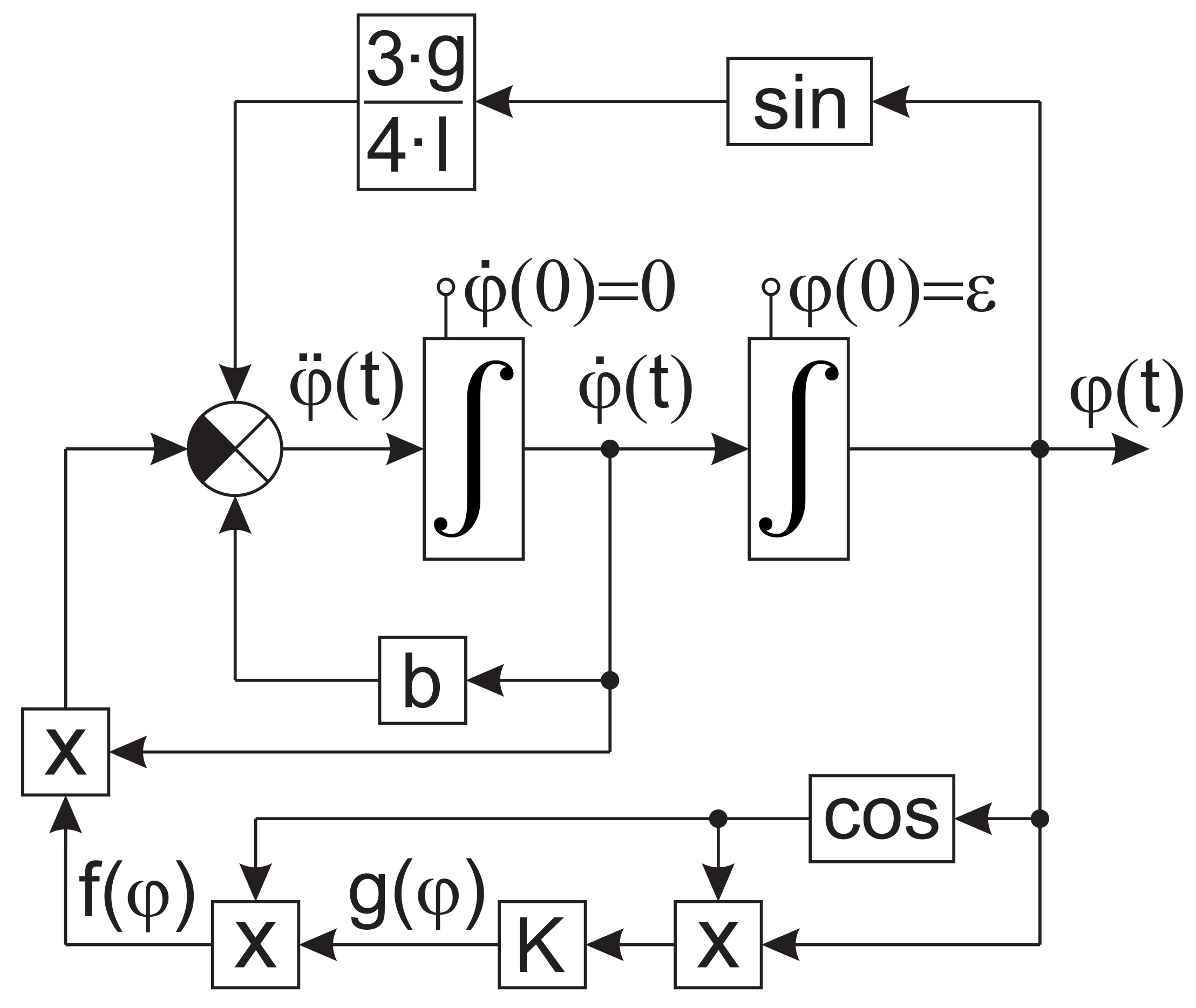
Figure 14 shows how a numerical solution $\phi (t)$ of Equation (14) is obtained considering $f(\phi )$ according to Equations (20) and (23).

Time-reversal symmetry function $\phi (T-t)$ is then used for computation of the reference control signal $u(t)$ according to

$$u(t)=-K·\phi (T-t)·cos[\phi (T-t)]·\dot{\phi }(T-t)·\frac{4}{3}·l.$$

(24)

Figure 15 shows how the found reference signal is applied for the inverted pendulum system in order to perform the swing-up from a lower stable position to the upright unstable position, see the initial values of the integrator, indicating its initial state.

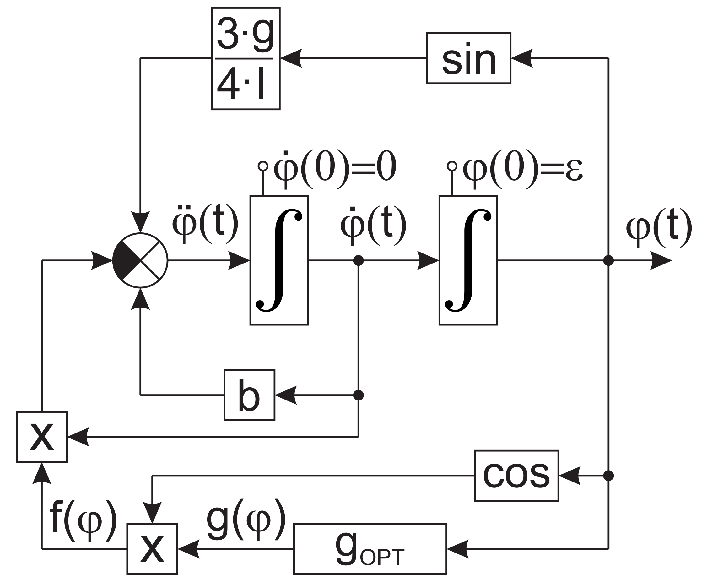
2.3.2. Calculation of $g(\circ )$ Function Based on Numerical Optimization Procedure

This approach extends the use of the proposed methodology for systems with one or more friction or damping terms, for example for double or triple inverted pendulums, or robotic systems with more arms. The explanation in this section will be provided for a single inverted pendulum.

The candidate function $g(\circ )$ may be expressed in many different forms. The shaping of this candidate function makes it possible to achieve the desired properties of the control and state trajectories. As an example, it may be naturally desired to achieve zero final values of cart position $x_3$ and its speed $x_4$.

The basic idea of using optimization procedure is to consider a finite number of individual free parameters, which define the candidate function $g(\circ )$. These parameters are pre-tuned by optimization algorithm with the use of certain cost function (see block $g_{OPT}$ in Figure 16). Note that the tuning is performed off-line as a separate process and that the values are used in the block scheme depicted in Figure 16.

The control and state trajectories are penalized during iterations of the procedure, and a minimum of the cost function is found. The cost function may reflect various requirements placed on properties of control and state trajectories, including constraints.

Here we present two different forms of the candidate function $g(\circ )$: trigonometric series and polynomial function.

In case of trigonometric candidate function we tested different numbers of harmonic components. Here we give a documentation of the obtained results using two components. The reason of using harmonic waves reflect the original expert choice and also requirements on properties such as a negative value around $\phi \approx 0$, a positive value around $\phi \approx \pi$. Furthermore, harmonic waves are close to the natural character of the pendulum and its oscillations. The candidate function is expressed as

$$g(\circ )=A_0+A_1·cos({\omega }_1·\circ +{\vartheta }_1)+A_2·cos({\omega }_2·\circ +{\vartheta }_2)$$

(25)

containing individual seven parameters: $A_0$, $A_1$, $A_2$, ${\omega }_1$, ${\omega }_2$, ${\vartheta }_1$, ${\vartheta }_2$.

In case of polynomial candidate function, it can be expressed according to

$$g(\circ )=A_0+A_1·\circ +A_2·{\circ }^2+A_3·{\circ }^3+A_4·{\circ }^4$$

(26)

containing the following individual five parameters: $A_0$, $A_1$, $A_2$, $A_3$, $A_4$.

The cost function used to determine how free parameters of $g(\circ )$ are tuned within $g_{OPT}$ block presented in Figure 16 in accordance with Equation (25) or with Equation (26) can be presented in form of

$$J=W_c·J_c+W_1·J_{x_1}+W_2·J_{x_2}+W_3·J_{x_3}+W_4·J_{x_4}+W_u·J_u$$

(27)

where $W_c$, $W_1$, $W_2$, $W_3$, $W_4$, $W_u$ are individual weighting coefficients for the components of the cost function and where

• Term $J_c$ penalizes violation of basic constraints placed on state trajectories and control;
• Term $J_{x_1}$ penalizes error between actual trajectory $x_1$ and predefined state trajectory $x_{1ref}$;
• The other terms $J_{x_2}$, $J_{x_3}$, $J_{x_4}$ penalize error of actual trajectories and predefined zero values at the final point of time interval;
• The last term $J_u$ is a stabilizing term assuring a converging solution, it represents energy minimization.

The control signal $u(t)$ is then computed via Equation (22) considering $g(\circ )$ in the form of Equation (25) or Equation (26). It uses a numerical solution $\phi (t)$ as presented in Figure 16.

3. Results for Primary Case Study

The presented case study documented the design of a control signal capable of the swing-up of the inverted pendulum on the cart. This kind of problem can be also considered as a special case of optimal control, with a cost function containing the Mayer term only, not the Lagrange term representing an integral path penalty. Therefore from a mathematical point of view, it is a TPBvP problem. Thus the resulting reference control signal and reference states are not optimal in terms of minimizing either time, fuel/energy, or any other respect. The time interval [0, T] over which the problem is solved, is chosen by an expert.

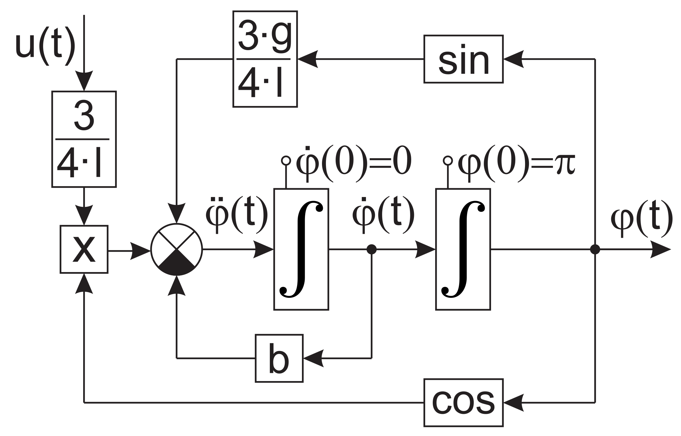
Note that the mathematical model used in this case consisted of a nonlinear differential equation containing two states representing the position of the pendulum and its speed. As the input signal represents a cart acceleration, the position and speed of the cart can be easily computed by a single or a double integrating as expressed as

$$v(t)={\int }_0^{t}u(\tau )d\tau$$

(28)

$$s(t)={\int }_0^{t}v(\tau )d\tau$$

(29)

Below documented time wave-forms use notation corresponding to the full state nonlinear model of the inverted pendulum on the cart according to

$$\left\{\begin{array}{c}{\dot{x}}_1(t)=x_2(t)\hfill \\ {\dot{x}}_2(t)=\frac{3g}{4l}·sin{x}_1(t)+\frac{3}{4·l}·u(t)·cos{x}_1(t)-b·x_2(t)\hfill \\ {\dot{x}}_3(t)=x_4(t)\hfill \\ {\dot{x}}_4(t)=u(t)\hfill \end{array}\right.$$

(30)

corresponding to $x_1(t)\equiv \phi (t)$, $x_2(t)\equiv \dot{\phi }(t)$, $x_3(t)\equiv s(t)$, $x_4(t)\equiv v(t)$ (compare to Figure 15 and Equations (28) and (29)).

The documentation of the results is divided into the sections, which correspond to the particular determination of $g(\circ )$ function in (22). Firstly there is a description of the results obtained via expert choice followed by the ones supported by the numerical optimization procedure.

3.1. Results Based on Expert Choice of $g(\circ )$ Function

Time-varying function describing coefficient of shear friction $f(\phi )$ given by Equation (20) depends on pendulum angle. Reasonable choice of function $g(\phi )$ in technical sense is such that for $\phi \in [0,\frac{\pi }{2}]$ friction is “negative” (in linguistic sense), i.e., movement of the pendulum rod is accelerated and for $\phi \in [\frac{\pi }{2},\pi ]$ the friction is “positive” (in linguistic sense), i.e., pendulum movement is slowed down. These requirements may be followed by $g(\phi )$ in the form of Equation (23). However this choice is not optimal in any technical sense.

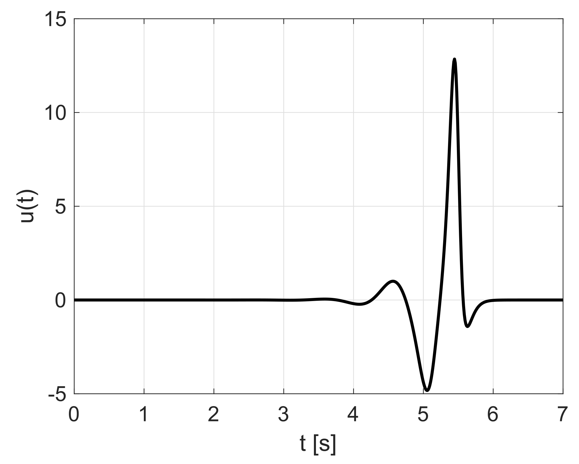
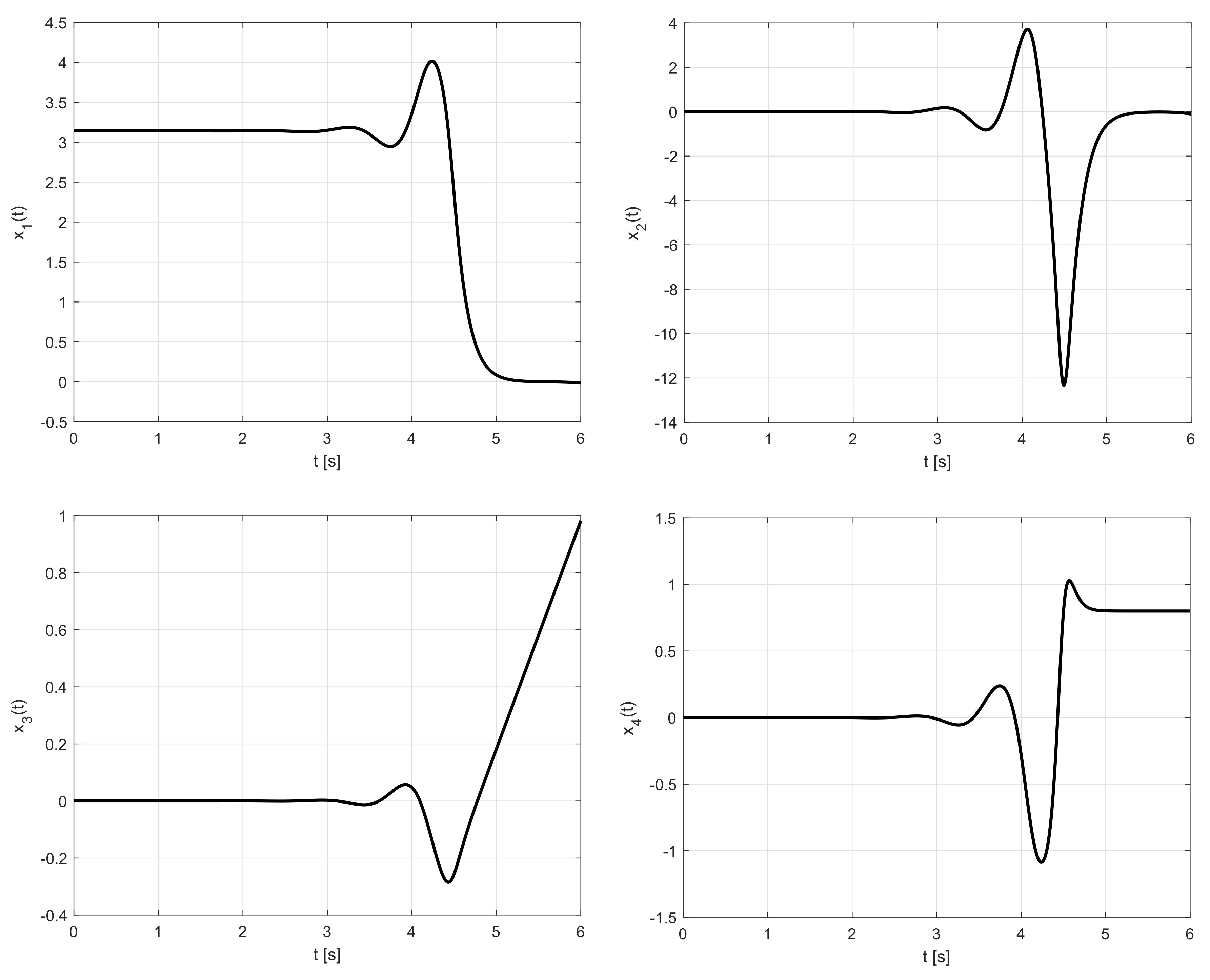
For documentation of particular results, the following values of the parameters were used: $g=10$, $l=0.15$, $b=0.07$, $K=2$, $T=6$. The computed reference control signal $u(t)$ used for the swing-up of the inverted pendulum on the cart found by the time-symmetry approach is shown in Figure 17.

The obtained corresponding reference states $x_1(t)$, $x_2(t)$, $x_3(t)$ and $x_4(t)$ are depicted in Figure 18.

From a technical point of view, the reference control signal and reference states represent open-loop control. These signals can be used in the feedback control structure of two degrees of freedom (2-DOF) type as described in [29] where the trajectory planning problem has been solved via the formulation of this problem as boundary value problem (BvP) with free parameters.

The feedback stabilization along the planned reference trajectory designed according to the proposed approach can be effectively implemented with the use of a time-varying LQR controller computed over a finite horizon. In other words, both the swing-up and stabilization in an upright position are performed within a closed-loop and by a single state feedback controller. The principle and functionality of such a closed-loop solution have been verified both in simulation and in practical operation with a real physical model, see [30] where the completely different method of trajectory planning has been applied, using numerical tools based on collocation methods.

The method of time-symmetry for trajectory planning proposed in this paper is unique authors’ work based on explicit mathematical background and on their professional experience.

The character of both reference control signal and reference states strongly depends on two crucial parameters: length of the time interval represented by the parameter T and expert-determined parameter K.

One of the main features of the proposed solution regarding the swing-up of the inverted pendulum is that the cart does not go back to its original (zero) position as seen in the above Figure 18.

Although it reaches up to almost one-meter deflection ($x_3$—position of the cart) at the final time according to simulation in open-loop, there can be several ways how to cope with this effect. Firstly, for a time it is possible to “ground” (set to zero) reference state $x_3(t)$ a bit earlier where the deflection is not so high and beyond the physical limit, letting the control error be compensated by feedback control in the closed-loop. Normally, for $t>T$, all the reference states, including $x_3$, are set to zero. However, regarding $x_3(t)$, it can also be kept in the last position. Secondly, the reference control and reference states can be used as a very good and precise initial guess of a newly formulated BvP problem that would handle all four state variables, and prescribe zero values at the final time for all states. This scenario was also tested successfully.

Third, adjusting of parameter K reduces this effect significantly. Generally, the lower the K value is, the more oscillatory the control signal and all reference states are, but the maximal amplitude of $x_3(T)$ rapidly goes to zero. For example, reducing $K=2$ to $K=1$, resp. $K=0.5$, causes $x_3(T)=0.4$ resp. $x_3(T)=0.05$ which are within usual physical limits (approximately $0.8-1$ m in case of typical single inverted pendulum models available on the market).

3.2. Results Based on the Numerical Optimization Procedure for $g(\circ )$ Function

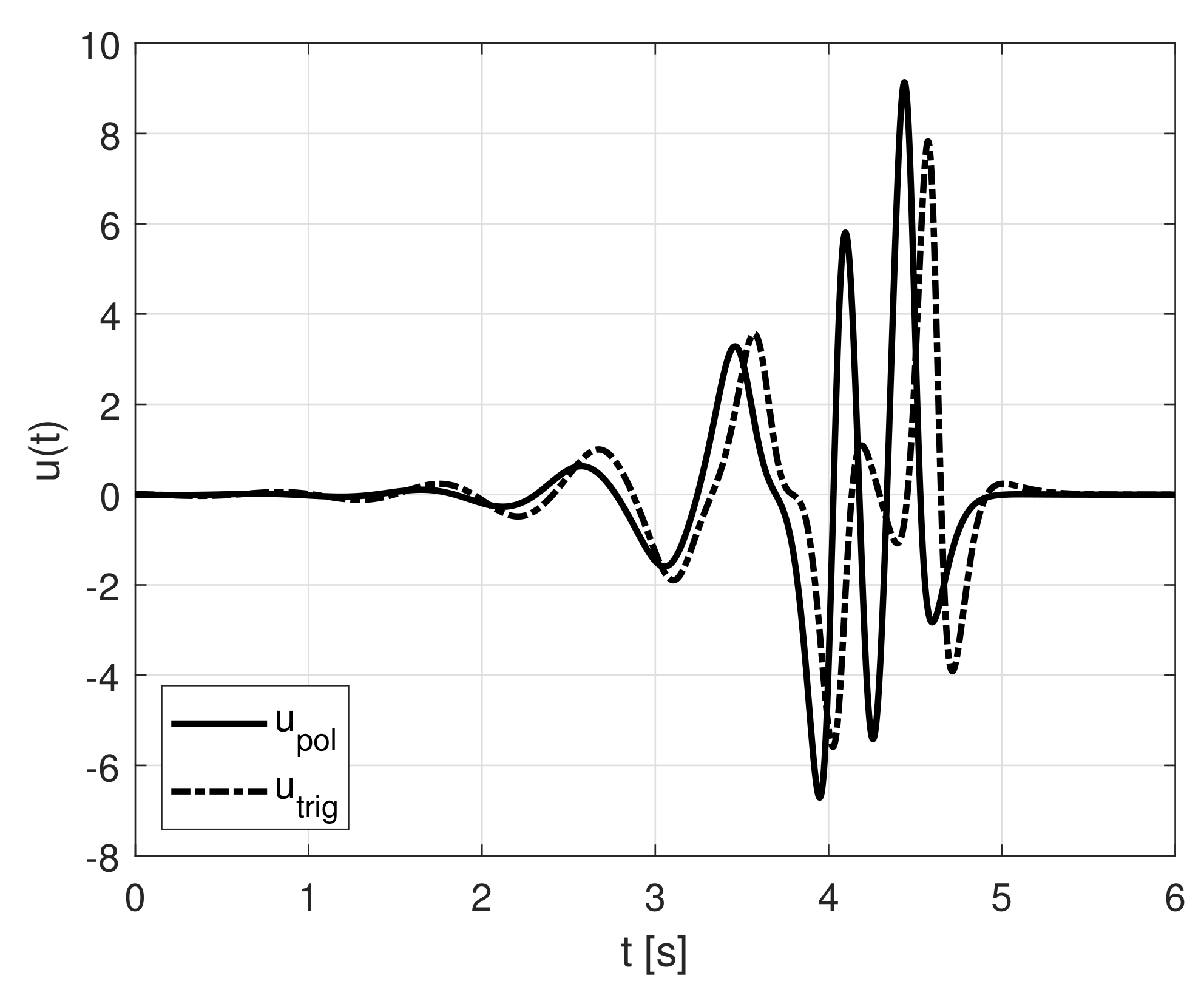
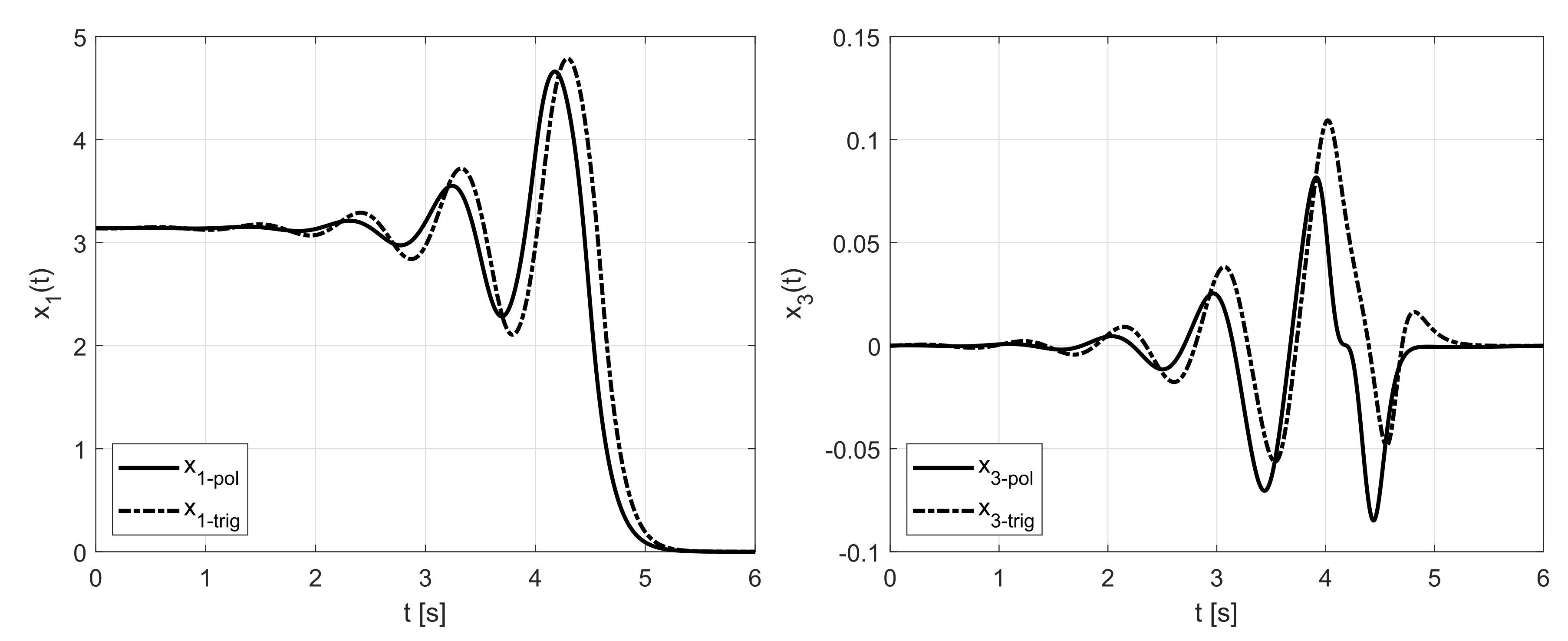
To prove effectiveness of numerical optimization procedure applied for $g(\circ )$ function, we introduce the waveforms of control signal $u(t)$ depicted in Figure 19, pendulum angle $x_1(t)$ and cart position $x_3(t)$ in Figure 20 both for trigonometric candidate (dashed line) and polynomial candidate (solid line).

The results in this section use the same parameters of the controlled system as in the previous section. The optimized parameters for $g(\circ )$ for trigonometric candidate according to Equation (25) are as follows:

• $A_0=0.5107$;
• $A_1=-1.1854$;
• ${\omega }_1=1.3606$;
• ${\vartheta }_1=4.6795$;
• $A_2=-1.7894$;
• ${\omega }_2=1.8575$;
• ${\vartheta }_2=4.0269$.

For polynomial candidate in accordance with Equation (26) the following optimized parameters were obtained:

• $A_0=0.2469$;
• $A_1=-2.9825$;
• $A_2=-0.1663$;
• $A_3=1.3260$;
• $A_4=-0.2716$.

Unlike in Figure 18, waveform $x_3(t)$ in Figure 20 shows that the cart moves back to original zero position as it was required. The combination of the proposed explicit methodology and numerical optimization preserves good quality of control signal and state trajectories, and also respects custom constraints placed on these signals.

4. Discussion

The proposed solution has been compared to a few different methods, obtained by third-party products aimed at solving of the optimal control problems, particularly in OptimTraj [31], ACADO [32], and PyTrajectory [33].

Different configurations of optimal control problems have been tried, including consideration of Lagrange term in a cost function. Although the originally proposed solution does not consider any constraints on particular states or any kind of Lagrange path penalization, it may be supported by a numerical optimization procedure as documented within the text. Choice of the three above mentioned software packages for comparison purposes was based on authors’ professional experience. The first one—OptimTraj is a very popular Matlab-based solution (library) usually applied for solving trajectory optimization problems, as it enables finding optimal trajectory for a dynamical system. The set trajectory enables the minimization of some cost function. The second tool applied for comparison purposes was ACADO, which is entirely developed in C++. Those two tools provide almost similar results, which allows the assumption that their results are reliable. Thus using them for comparison purposes is rational. The last tool method is PyTrajectory, which is applied for trajectories design for states transitions in non-linear systems, to which group inverted pendulum belongs. The very interesting fact about PyTrajectory is that it does not allow time step below 10 ms. With this period, the computed reference trajectories can be considered as worst-case yet the time-varying state controller enables to deal with such situation in an appropriate way. The comparison was done in a qualitative technical sense and it is beyond the scope of this paper. A strict quantitative comparison with the mentioned software tools using some performance index would require the identical formulation of the optimization task, which is impossible due to the unique character of the proposed methodology and due to the kind of formulation these tools use. The computed solution shows very favorable features in terms of the character of the waveforms and also of the maximal amplitudes of the reference control signal, which is usually an issue when other numerical software tools mentioned above are used. The main reason for this good quality is that the found solution is based on a natural motion of the pendulum, obtained by experiment considering a free uncontrolled swing-down. Note that all waveforms shown in Figure 18 and Figure 20 were obtained by open-loop simulation using particular control signal $u(t)$. It can be seen that there is no deflection between the prescribed and simulated values at the final time. This zero or negligible deflection is practically impossible to achieve when using a different approach to trajectory planning. Although BvP is solved successfully with a given precision, a numerical model-based simulation using the reference control signal as the input is a different question. The main reason for this phenomenon is that the system is highly nonlinear and unstable. Thus the open-loop experiments usually suffer from deflections between computed states and simulated states already in the simulation phase. It usually manifests as a significant non-zero error in the final time point $t=T$ as the error has a cumulative character over time. Thorough literature study performed by the authors of this work prove that no similar solutions have been applied so far and that the obtained results were satisfactory and improved the area of the study.

5. Conclusions

Above Figure 18 and Figure 20 were obtained by open-loop simulation using particular control signal $u(t)$, $t=T$. The general idea presented in this paper can be used in the problem of trajectory planning, particularly in so-called finite-time transition problems where the system must be transferred from a given initial state to another in the finite time, see [34].

Apart from a basic motivational case study of the linear mass-spring-damper model, the paper also presents an integral thorough approach of efficient trajectory planning applied for a single inverted pendulum, which is nonlinear, unstable, non-minimum phase and underactuated system. Plans for future work in particular cover applications for double or possibly triple pendulums. However, it is also planned to create general methodology, which would allow implementing this approach in any mechanical system described by analytical equations of motion under the presence of damping or friction.

Through analysis of mathematical background related to the proposed in this paper solution allowed to conclude that the existence of the designed control signal and state trajectories is guaranteed if the equations of the motion have a solution in the direct flow of time.

Further Research Plans

As it was discussed in this paper proposed method could be applied for the purposes of trajectory planning and solving of the TPBvP. Plans for future work cover also potential applications for double and possibly triple pendulums. Further research plans include the development of general methodology, which would allow implementing the approach presented in this work in any mechanical system described by analytical equations of motion under the presence of damping or friction. Thus the authors of this work would like to pursue this research topic in the near future. Further research will include the implementation of more advanced smoothing filters for the purpose of pendulums’ trajectories improvement. Some of the initial studies based on single inverted pendulums have been already carried out and in detail and presented in [25]. Another interesting topic would be the development of reference trajectories for the efficient fractional controller for single-, double- and triple-pendulums, which may have a positive effect on the systems’ stabilisation [35,36].

References

- Betts, J.T. Survey of numerical methods for trajectory optimization. J. Control Guid. Dyn. 1998, 21, 193–207. [Google Scholar] [CrossRef]
- Powers, D.L. Boundary Value Problems; Harcourt Brace Jovanovich: San Diego, CA, USA, 1987. [Google Scholar]
- Keller, H. Numerical Methods for Two-Point Boundary Value Problems; Blaisdell Publishing Co.: Waltham, MA, USA, 1987. [Google Scholar]
- Press, W.H.; Teukolsky, S.A.; Vetterling, W.T.; Flannery, B.P. Numerical Recipes in C, the Art of Scientific Computing, 2nd ed.; Cambridge University Press: Cambridge, UK, 1992. [Google Scholar]
- Guibout, V.; Scheeres, D.J. Solving two-point boundary value problems using generating functions: Theory and applications to astrodynamics. In Elsevier Astrodynamics Series; Gurfil, P., Ed.; Butterworth-Heinemann: Oxford, UK, 2006; Volume 1, pp. 53–105. [Google Scholar]
- Lamb, J.; Roberts, J. Time-reversal symmetry in dynamical systems: A survey. Phys. Nonlinear Phenom. 1998, 112, 1–39. [Google Scholar] [CrossRef]
- Contessa, G. Scientific models and fictional objects. Synthese 2010, 172, 215. [Google Scholar] [CrossRef]
- Nelson, R.A.; Olsson, M. The pendulum—Rich physics from a simple system. Am. J. Phys. 1986, 54, 112–121. [Google Scholar] [CrossRef]
- Furuta, K.; Iwase, M. Swing-up time analysis of pendulum. Bull. Pol. Acad. Sci. Tech. Sci. 2004, 52, 153–163. [Google Scholar]
- Birkhoff, G.D. The restricted problem of three bodies. Rendiconti del Circolo Matematico di Palermo (1884–1940) 2008, 39, 265. [Google Scholar] [CrossRef] [Green Version]
- DeVogelaere, R. On the structure of periodic solutions of conservative systems, with applications. In Contribution to the Theory of Nonlinear Oscil Lations; Lefschetz, S., Ed.; Princeton University Press: Princeton, NJ, USA, 1958; Volume 4, pp. 53–84. [Google Scholar]
- Heinbockel, J.; Struble, R. Periodic solutions for differential systems with symmetries. J. Soc. Industr. Appl. Math. 1965, 13, 425–440. [Google Scholar] [CrossRef]
- Moser, J. Convergent series expansions for quasi-periodic motions. Math. Annalen 1967, 169, 136–176. [Google Scholar] [CrossRef]
- Bibikov, Y.; Pliss, V. On the existence of invariant tori in a neighbourhood of the zero solution of a system of ordinary differential equations. Differ. Equ. 1967, 3, 967–976. [Google Scholar]
- Hale, J. Ordinary differential equations. In Pure and Applied Mathematics; Wiley-Interscience: New York, NY, USA, 1969; Volume 21. [Google Scholar]
- Devaney, R. Reversible diffeomorphisms and flows. Trans. Am. Math. Soc. 1976, 218, 89–113. [Google Scholar] [CrossRef]
- Arnol’d, V.; Sevryuk, M. Nonlinear phenomena in plasma physics and hydrodynamics. In Pure and Applied Mathematics; Sagdeev, R., Ed.; Mir: Moscow, Russia, 1986; Volume 21, pp. 31–64. [Google Scholar]
- Miller, D.J. Realism and time symmetry in quantum mechanics. Phys. Lett. 1996, 222, 31–36. [Google Scholar] [CrossRef]
- Aharonov, Y.; Tollaksen, J. New insights on time-symmetry in quantum mechanics. arXiv 2007, arXiv:0706.1232. [Google Scholar]
- Vlad, S.E. Boolean Functions: Topics in Asynchronicity, 1st ed.; Wiley: New York, NY, USA, 2019. [Google Scholar] [CrossRef]
- Knoll, C.; Röbenack, K. Trajectory planning for a non-flat mechanical system using time-reversal symmetry. PAMM 2011, 11, 819–820. [Google Scholar] [CrossRef]
- Stannarius, R. Time reversal of parametrical driving and the stability of the parametrically excited pendulum. Am. J. Phys. 2009, 77, 164–168. [Google Scholar] [CrossRef]
- Kerr, W.; Williams, M.; Bishop, A.; Fesser, K.; Lomdahl, P.; Trullinger, S. Symmetry and chaos in the motion of the damped driven pendulum. Z. FüR Phys. Condens. Matter 1985, 59, 103–110. [Google Scholar] [CrossRef]
- Roberts, J.; Quispel, G. Chaos and time-reversal symmetry. Order and chaos in reversible dynamical systems. Phys. Rep. 1992, 216, 63–177. [Google Scholar] [CrossRef]
- Kawala-Sterniuk, A.; Zolubak, M.; Ozana, S.; Siui, D.; Macek-Kaminska, K.; Grochowicz, B.; Pelc, M. Implementation of smoothing filtering methods for the purpose of improvement inverted pendulum’s trajectory. Prz. Elektrotech 2019. [Google Scholar] [CrossRef]
- Limebeer, D.J.N.; Massaro, M. Dynamics and Optimal Control of Road Vehicles; Oxford University Press: Oxford, UK, 2018. [Google Scholar]
- Hatano, N.; Ordonez, G. Time-reversal symmetry and arrow of time in quantum mechanics of open systems. Entropy 2019, 21, 380. [Google Scholar] [CrossRef] [Green Version]
- Yokoyama, J.; Mihara, K.; Suemitsu, H.; Matsuo, T. Swing-up control of a inverted pendulum by two step control strategy. In Proceedings of the 2011 IEEE/SICE International Symposium on System Integration (SII), Kyoto, Japan, 20–22 December 2011; pp. 1061–1066. [Google Scholar] [CrossRef]
- Ozana, S.; Schlegel, M. Computation of reference trajectories for inverted pendulum with the use of two-point BvP with free parameters. IFAC-PapersOnLine 2018, 51, 408–413. [Google Scholar] [CrossRef]
- Ozana, S. Swing-Up and Control of Linear Simple Inverted Pendulum. 2018. Available online: https://youtu.be/Sqhr8fYhMfg (accessed on 5 May 2020).
- Kelly, M. An introduction to trajectory optimization: How to do your own direct collocation. SIAM Rev. 2017, 59, 849–904. [Google Scholar] [CrossRef]
- Houska, B.; Ferreau, H.; Diehl, M. ACADO Toolkit – an open source framework for automatic control and dynamic optimization. Optim. Control. Appl. Methods 2011, 32, 298–312. [Google Scholar] [CrossRef]
- Kunze, A. Pytrajectory’s Documentation. 2005. Available online: https://pytrajectory.readthedocs.io (accessed on 5 May 2020).
- Graichen, K.; Hagenmeyer, V.; Zeitz, M. A new approach to inversion-based feedforward control design for nonlinear systems. Automatica 2005, 41, 2033–2041. [Google Scholar] [CrossRef]
- Dwivedi, P.; Pandey, S.; Junghare, A.S. Stabilization of unstable equilibrium point of rotary inverted pendulum using fractional controller. J. Frankl. Inst. 2017, 354, 7732–7766. [Google Scholar] [CrossRef]
- Mandić, P.D.; Lazarević, M.P.; Šekara, T.B. Stabilization of inverted pendulum by fractional order PD controller with experimental validation: D-decomposition approach. In Proceedings of the International Conference on Robotics in Alpe-Adria Danube Region, Belgrade, Serbia, 30 June–2 July 2016; pp. 29–37. [Google Scholar]
Figure 1.
State-space scheme of the mass-spring-damper model.
Figure 2.
Simulation experiment: obtaining a response to initial conditions.
Figure 3.
Simulation experiment: a response to initial conditions according to Figure 2.
Figure 4.
Simulation experiment: Adding an artificial damping to the system and storing signal .
Figure 6.
Simulation experiment: damping compensation by signal .
Figure 7.
Simulation experiment: application of time-reversing control signal (t).
Figure 8.
Simulation experiment: output of the system according to Figure 7.
Figure 9.
Simulation experiment: elimination of damping effect.
Figure 10.
Simulation experiment: application of the computed control signal to the original system.
Figure 11.
The output signal according to Figure 10.
Figure 12.
The waveform of control signal .
Figure 13.
Situation scheme of the system.
Figure 14.
Simulation experiment: numerical solution .
Figure 15.
Simulation experiment: application of the reference control signal to perform the swing-up.
Figure 16.
Figure 17.
Reference control input signal .
Figure 18.
Reference trajectories: , , , .
Figure 19.
Figure 20.
Reference trajectories: , .
© 2020 by the authors. Licensee MDPI, Basel, Switzerland. This article is an open access article distributed under the terms and conditions of the Creative Commons Attribution (CC BY) license (http://creativecommons.org/licenses/by/4.0/).
Share and Cite
MDPI and ACS Style
Ozana, S.; Docekal, T.; Kawala-Sterniuk, A.; Mozaryn, J.; Schlegel, M.; Raj, A. Trajectory Planning for Mechanical Systems Based on Time-Reversal Symmetry. Symmetry 2020, 12, 792. https://0-doi-org.brum.beds.ac.uk/10.3390/sym12050792
AMA Style
Ozana S, Docekal T, Kawala-Sterniuk A, Mozaryn J, Schlegel M, Raj A. Trajectory Planning for Mechanical Systems Based on Time-Reversal Symmetry. Symmetry. 2020; 12(5):792. https://0-doi-org.brum.beds.ac.uk/10.3390/sym12050792
Chicago/Turabian StyleOzana, Stepan, Tomas Docekal, Aleksandra Kawala-Sterniuk, Jakub Mozaryn, Milos Schlegel, and Akshaya Raj. 2020. "Trajectory Planning for Mechanical Systems Based on Time-Reversal Symmetry" Symmetry 12, no. 5: 792. https://0-doi-org.brum.beds.ac.uk/10.3390/sym12050792
Note that from the first issue of 2016, this journal uses article numbers instead of page numbers. See further details here.