Model Reduction for Kinetic Models of Biological Systems


1
Department of Mathematics and Computer Science, Freie Universität Berlin, 14195 Berlin, Germany
2
Department of Mathematics, Arish University, 31111 Arish, North Sinai, Egypt
3
Department of Mathematics, Technische Universität Berlin, 10623 Berlin, Germany
*
Author to whom correspondence should be addressed.
Symmetry 2020, 12(5), 863; https://0-doi-org.brum.beds.ac.uk/10.3390/sym12050863
Submission received: 16 March 2020
/
Revised: 3 May 2020
/
Accepted: 6 May 2020
/
Published: 25 May 2020
(This article belongs to the Special Issue Mathematical Modeling and Computational Methods in Science and Engineering II)
Abstract
:High dimensionality continues to be a challenge in computational systems biology. The kinetic models of many phenomena of interest are high-dimensional and complex, resulting in large computational effort in the simulation. Model order reduction (MOR) is a mathematical technique that is used to reduce the computational complexity of high-dimensional systems by approximation with lower dimensional systems, while retaining the important information and properties of the full order system. Proper orthogonal decomposition (POD) is a method based on Galerkin projection that can be used for reducing the model order. POD is considered an optimal linear approach since it obtains the minimum squared distance between the original model and its reduced representation. However, POD may represent a restriction for nonlinear systems. By applying the POD method for nonlinear systems, the complexity to solve the nonlinear term still remains that of the full order model. To overcome the complexity for nonlinear terms in the dynamical system, an approach called the discrete empirical interpolation method (DEIM) can be used. In this paper, we discuss model reduction by POD and DEIM to reduce the order of kinetic models of biological systems and illustrate the approaches on some examples. Additional computational costs for setting up the reduced order system pay off for large-scale systems. In general, a reduced model should not be expected to yield good approximations if different initial conditions are used from that used to produce the reduced order model. We used the POD method of a kinetic model with different initial conditions to compute the reduced model. This reduced order model is able to predict the full order model for a variety of different initial conditions.
1. Introduction
In biological systems, kinetic models of biochemical networks are necessary for predicting and optimizing the behavior of cells in culture. Most of these models are high-dimensional and involve a large number of reactions and species and reaction rate constants of widely different orders of magnitude [1]. Thus, model order reduction (MOR) is considered to be a vital topic and essential for an efficient numerical simulation. In general, model order reduction is a mathematical theory for reducing the computational complexity of large-scale dynamical systems via finding a low-dimensional approximation while preserving the most important information of the full order system. The computational complexity of a method is a measure of time or storage space that the method requires to solve a given task. In this paper, we reduce the time cost of the simulation of dynamical systems using MOR methods, as we will discuss later; see Section 3. Moreover, MOR methods of a higher order dimensional system produce a lower order dimensional system, which is considered more efficient for reducing the computational effort in mathematical processes, e.g., an optimization process.
The model reduction method has been discussed in mathematical modeling of biological systems. Here, Michaelis–Menten kinetics [2,3], whose derivation is based on a quasi-steady state assumption [4,5], is considered the famous example of the model reduction theory of enzymatic reactions. Many other model reduction methods [6] have been discussed that are based on different ways of analyzing the system. Sensitivity analysis [7,8] is based on eliminating parameters that are noticed to be the least sensitive in affecting the model. The lumping method was initially presented in the 1960s by Wei and Kuo [9,10]. The idea behind the lumping method is to remove a group of state variables from the system and replace them with a new dynamical variable (lumped), which is related to the original system by lumping functions [11,12]. Time scale analysis [13] is the most recent model reduction approach that is used in biological systems. It assumes two time scales, fast and slow, whereby the fast one converges to a quasi-steady state. However, in some cases, the differences in the time scales do not suffice for obtaining a reduced model that behaves in the same way as the original model [14]. Thus, the required conditions of Tikhonov’s theorem (see [15,16]) should be satisfied to apply the model order reduction method. In [17], the model reduction of a small single metabolic-genetic network was studied using the time scale separation. The model reduction of a two-stage anaerobic digestion process model was also studied in [18], and the model reduction of RNA polymerase was studied in [19].
The conditions that have to hold for the applicability of Tikhonov’s theorem are not trivial, especially for a large-scale dynamical system. Therefore, we aim to apply another popular approach for model reduction: the proper orthogonal decomposition (POD), a method that aims at obtaining low-dimensional approximate descriptions of high-dimensional systems while preserving important information. The POD method, also known as Karhunen–Loève Expansion (KLE) [20,21], is based on the idea of projecting the full order system onto a lower dimensional subspace while capturing the main characteristics of the system. Within the POD method, the key idea is to use singular value decomposition (SVD) [22,23,24] to calculate the basis for the low-dimensional subspace. The SVD is considered to be one of the most important matrix factorizations in the field of data science, since it exists for any matrix and can be used for approximating high-dimensional data by low-dimensional data in terms of dominant patterns.
A drawback of the POD method is that for time-dependent and/or parameterized nonlinear systems, the computational complexity for evaluating the nonlinear term in the reduced order model remains that of the original problem, although the dimension of the system is reduced. The discrete empirical interpolation method (DEIM) was proposed in [25] for high-dimensional nonlinear ODE models and is able to greatly improve the dimension reduction efficiency of the POD method.
In this paper, we discuss the model order reduction techniques by POD and DEIM for kinetic models of biological systems. From a practical point of view, the POD and DEIM methods are more advantageous for large-scale dynamical systems than time scale separation techniques, since we do not have to take care of satisfying the conditions required, e.g., for Tikhonov’s theorem.
The methods are applied to a kinetic model of a metabolic-genetic network that was introduced in [26]. In addition, we apply the approaches to different models of biological systems from the BioModels database (http://identifiers.org/biomodels.db), and we compare the time costs of the simulation for the original and the reduced order model in different cases. The MOR methods depend on a snapshot matrix generated from numerical simulations of the dynamical system with certain initial conditions. In general, a reduced model should not be expected to yield good approximations if different initial conditions are used from those used to produce the reduced order model [27].
However, an important characteristic of a kinetic model in systems biology is that it can predict different scenarios of behavior for the system that can be stimulated by prescribing different initial conditions. Here, we use the POD approach to compute a reduced order model of a kinetic model for different initial conditions of the dynamical system. This reduced order model is able to predict the full order model for a variety of different initial conditions. Using different initial conditions in the time scale separation technique will usually fail, since the algebraic equations of the fast variables may not be solvable if inconsistent initial values are prescribed; see [17].
The remainder of this paper is organized in the following manner. We discuss the model reduction of a dynamical system using POD and DEIM in Section 2. We then apply the approaches to a simplified metabolic-genetic network and to different kinetic models from the BioModels database in Section 3. We study the POD method of a kinetic model with different initial conditions in Section 4. Finally, we end with some concluding remarks in Section 5.
2. Proper Orthogonal Decomposition for Differential Equations
We consider a system of ordinary differential equations that is given by:
where is the m-dimensional state vector of the model and f is a nonlinear function mapping from to the m-dimensional space depending on parameters . Moreover, denotes the number of parameters, and is a given initial value.
The proper orthogonal decomposition (POD) method is a projection-based order reduction technique that aims at constructing a reduced order system of order approximating the original system (1) from a subspace that is spanned by a reduced basis of dimension k in using Galerkin projection. Let denote a matrix whose orthonormal columns form the reduced POD basis, then the reduced system of (1) is obtained by replacing in (1) by , and projecting the system (1) onto to get:
In the POD approach, a reduced basis is constructed from a truncated singular value decomposition (SVD) of a matrix of sample trajectory vectors (snapshots), assuming that the samples are on or near the attracting low-dimensional manifold that represents the solution space.
We introduce the trajectory snapshot matrix consisting of a time series of data (samples of trajectories) and assume that . This snapshot matrix can be obtained via a numerical solution of the dynamical system or from measured datasets. The SVD guarantees the existence of real non-negative numbers and orthogonal matrices with columns and with columns such that:
where and the zeros denote matrices of appropriate dimensions. Similarly, we have:
Then, the POD basis is given by . We set , and the linear span of the vectors determines the best rank-k approximation of in the sense that is minimizes the two-norm of the approximation error:
see [28]. In this truncation of the SVD, we try to approximate the matrix with k chosen as small as possible, but as large as necessary to obtain a good approximation. The strong decay of singular values allows a good representation with only a few modes. If the decay of singular values is gradual, one is forced to use a high number of modes to get a good approximation.
The general philosophy in model order reduction is to cut off singular values with , where is chosen such that a (much) smaller number of basis elements is sufficient to capture the main features of the solution of (1). The goal is to choose k small enough, while the relative information content [29] of the basis for the k-dimensional subspace, defined by:
is near one. If the k-dimensional subspace should contain a percentage p of the information contained in the full-dimensional space , then one should choose k such that:
see [29].
A drawback of the POD method is the computational complexity for time-dependent and/or parameterized nonlinear systems. Although the dimension of the system is reduced in the sense that far fewer variables are present in the reduced order system (2), the complexity of evaluating the nonlinear term remains that of the original problem. The nonlinear term:
in the reduced system (2) has a computational complexity that depends on m, the dimension of the original full-order system (1), and in particular, it requires a full evaluation of the nonlinear function f at the m-dimensional vector , such that solving this system is still as costly as solving the original system.
The discrete empirical interpolation method (DEIM) was proposed in [25] for high-dimensional nonlinear ODE models to improve greatly the dimension reduction efficiency of POD with Galerkin projection by approximating the nonlinear function by combining projection with interpolation.
The nonlinear function is approximated by projecting it onto a subspace spanned by a POD basis of dimension . This POD basis for the nonlinear function is constructed by applying the POD to the nonlinear snapshot matrix obtained from the original full order model (1), where and with . The values in are already needed to generate the snapshot matrix , and thus, it requires no additional cost other than the truncated SVD to obtain . Similar as above, the two-norm error for the approximation of the nonlinear function is given by:
where , , , and denotes the singular values of ; again, see [28].
The corresponding POD-DEIM reduced system is designed by applying Galerkin projection on the space spanned by the columns of the POD basis matrix and then applying the DEIM approximation to the nonlinear function using interpolation projection onto the columns space of the POD basis matrix . The resulting reduced system is then given by:
where and is a matrix whose columns come from some selected columns of the identity matrix corresponding to the so-called DEIM indices. In more detail, the nonlinear function in (2) approximated by DEIM can be written as:
such that the nonlinear term (5) can be approximated by:
The first term does not depend on t and can be precomputed before solving the system of ODEs. The interpolation indices used in the construction of the matrix where is the columns of the identity matrix for , are selected inductively from the basis by the DEIM algorithm; see [25]. By using the DEIM algorithm, it is guaranteed that is always nonsingular.
Note that the DEIM approximation is uniquely determined by the projection matrix , and is an interpolation approximation for the original function f, since is exact at the interpolation indices, i.e., it holds that for all .
DEIM solves the computational complexity problem that occurs since the nonlinear term has to be evaluated by replacing the orthogonal projection of POD with an interpolatory projection. As a result, the nonlinear term has to be assessed only at a few selected component functions, which greatly reduces the complexity. Note that the choice of the snapshots is a crucial factor in the construction of the POD basis, and the choice of the projection basis greatly affects the accuracy of the approximation of the original solution space. The snapshots are numerically sampled values of the trajectory at particular time steps for a particular initial condition and at particular parameter values. The DEIM state approximation error for large systems of nonlinear ODEs was analyzed in [28], and a bound on the global state space approximation error was provided.
3. Application of the POD-DEIM Approach to Kinetic Model Examples
In this section, we apply the POD-DEIM model reduction method introduced in the previous section to kinetic models for different examples of biological systems. In particular, we consider the simple metabolic-genetic network example of [26], a large-scale kinetic model of the yeast metabolic network taken from [30], and a large-scale kinetic model of the Escherichia coli metabolic network introduced in [31]. All results presented in the following sections were computed with MATLAB (R2017a) on a GNU Linux system (openSUSE Leap 15.0).
3.1. Kinetic Model of the Metabolic-Genetic Network
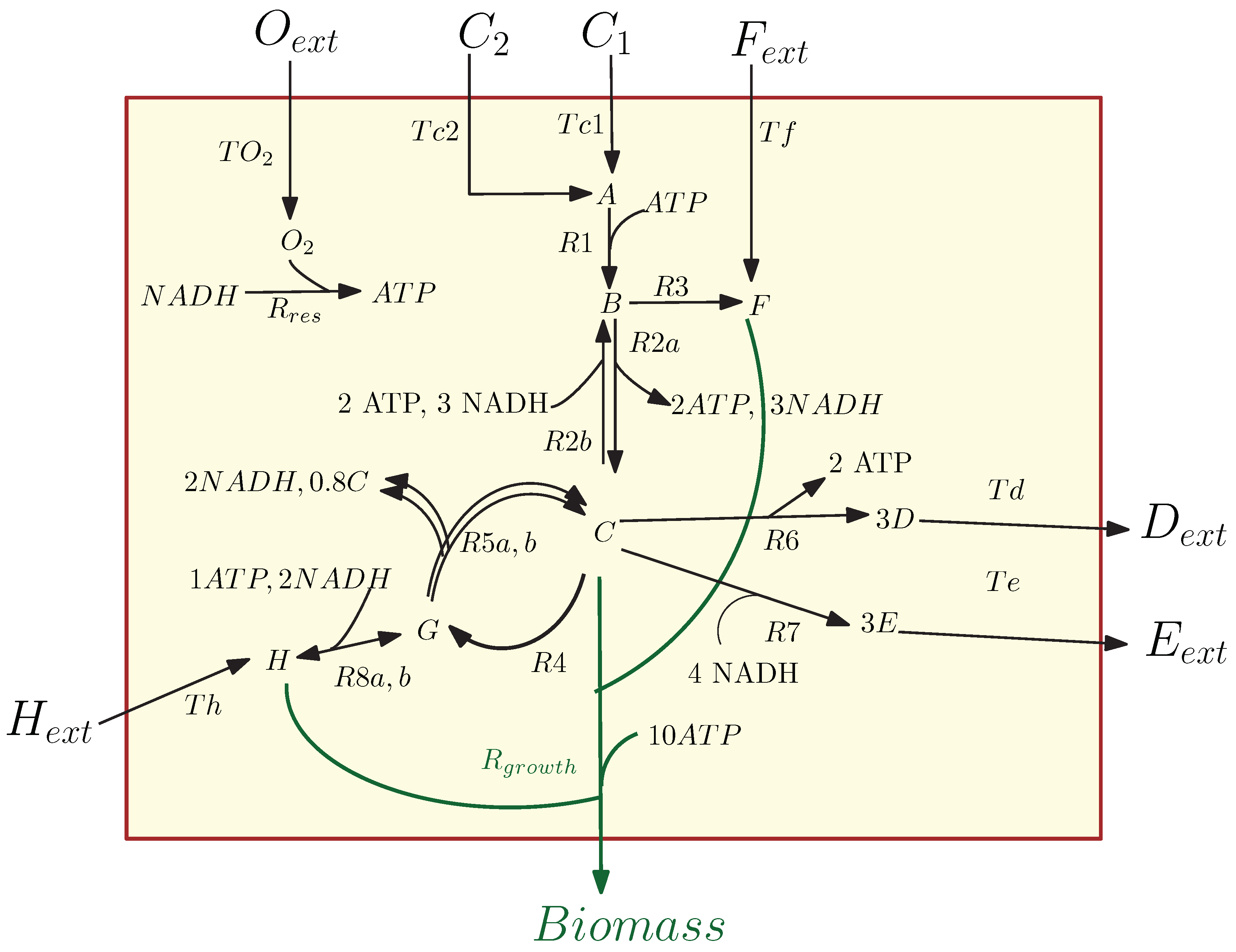
In this example, we consider the model of the simple metabolic-genetic network studied in [26]; see Figure 1. The network contains 20 reactions and 19 dynamic states: 7 external metabolites , 11 internal metabolites , and biomass. This sample metabolic network models the dynamic growth of a cell while seven of the reactions are regulated by four temporary regulatory constraints, and it can be used to illustrate several insightful scenarios (e.g., preferential carbon source uptake/catabolite repression, anaerobic growth, amino acid biosynthesis pathway repression, or transcriptional regulation to maintain the concentration levels of important metabolites; see [26]). For this metabolic network example, we introduced a kinetic model describing the dynamics of external metabolites, internal metabolites, and regulatory rules for the network; see the Appendix A.
In particular, the change of the external metabolite concentrations in the cell medium generates different scenarios. Here, we will discuss the two scenarios called the diauxic-switch and aerobic/anaerobic-diauxie scenarios, which were also studied in [26]. First, we apply MOR methods to the kinetic model of the metabolic genetic network (A2) in the diauxic-switch scenario.
Application of POD-DEIM to the Diauxic-Switch Scenario
In the case of the diauxic-switch scenario, there are two sources of carbon that are introduced to the cell. During the first phase, the cells prefer to metabolize the sugar on which they can grow faster (e.g., ). When the first sugar has been exhausted, the cells switch to the second source of carbon (e.g., ); see [32,33].
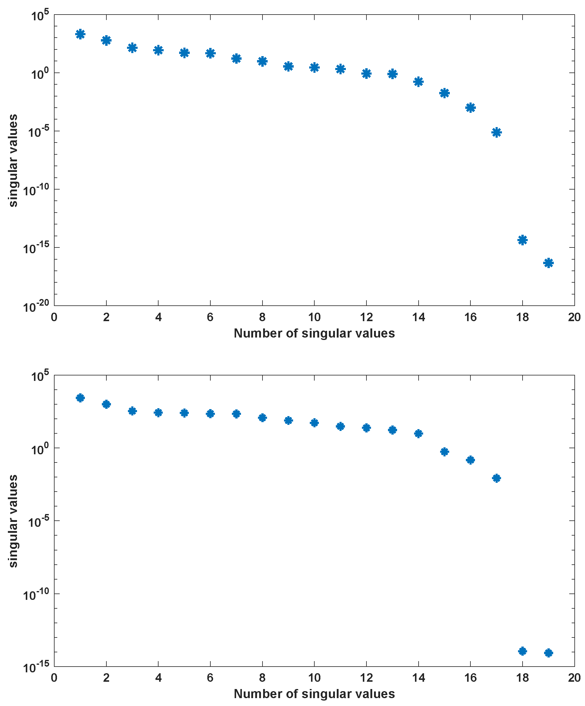
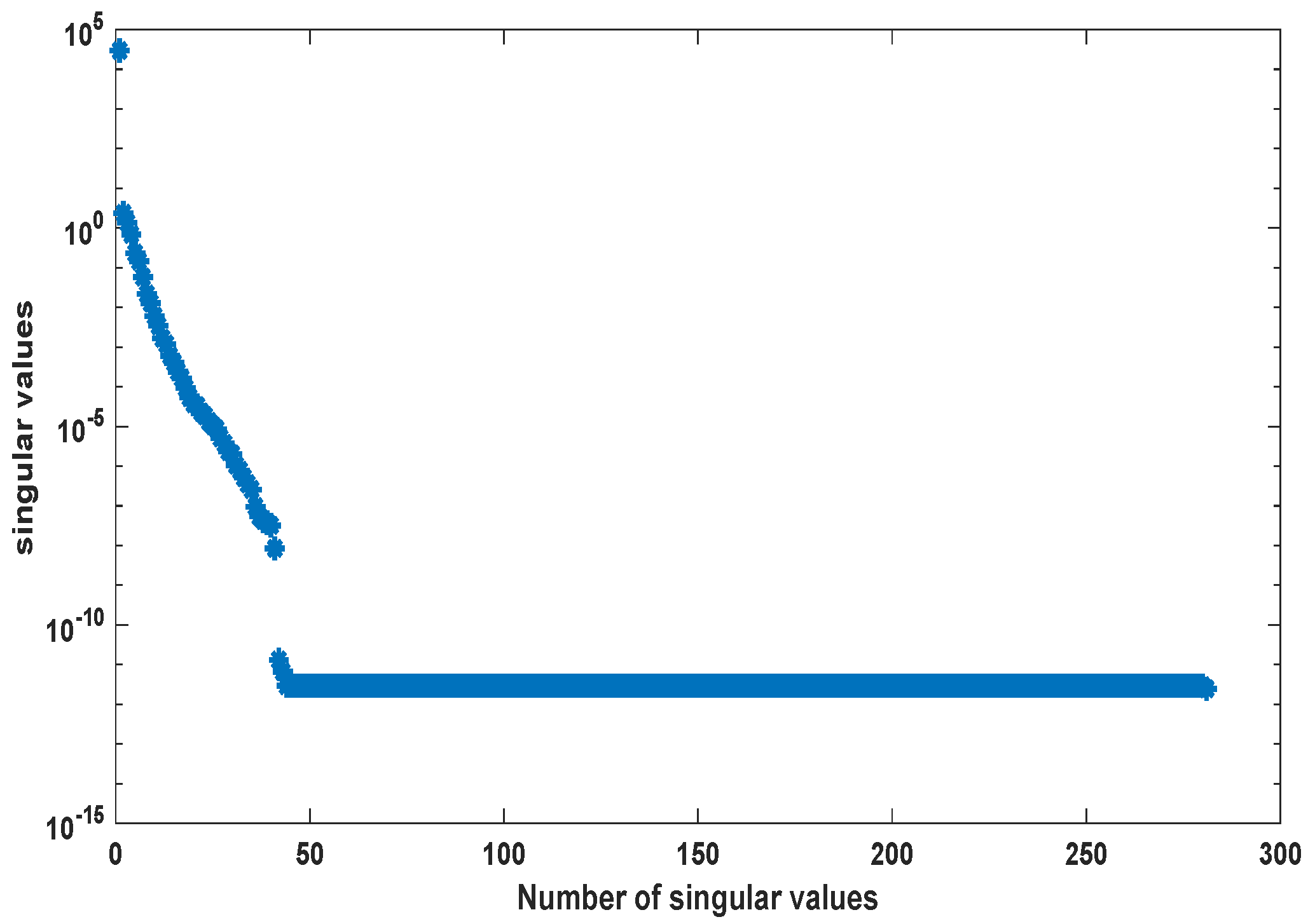
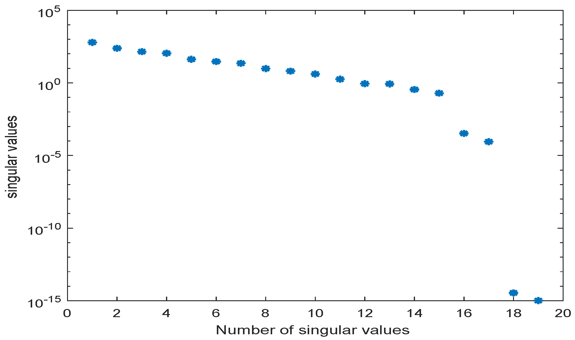
We use the MATLAB function ode23s with tolerances to compute a numerical solution of the ODE system (A2) with parameters as given in Table A2 in the time interval [0, 5] hr using a non-equidistant output time-grid. The initial concentrations of internal metabolites are assumed to be . The initial concentrations of external metabolites are taken from [26] for the different scenarios. This numerical solution yields the snapshot matrix and the nonlinear snapshot matrix . We used the MATLAB function svd to calculate the singular value decomposition of and . The singular values are depicted in Figure 2.
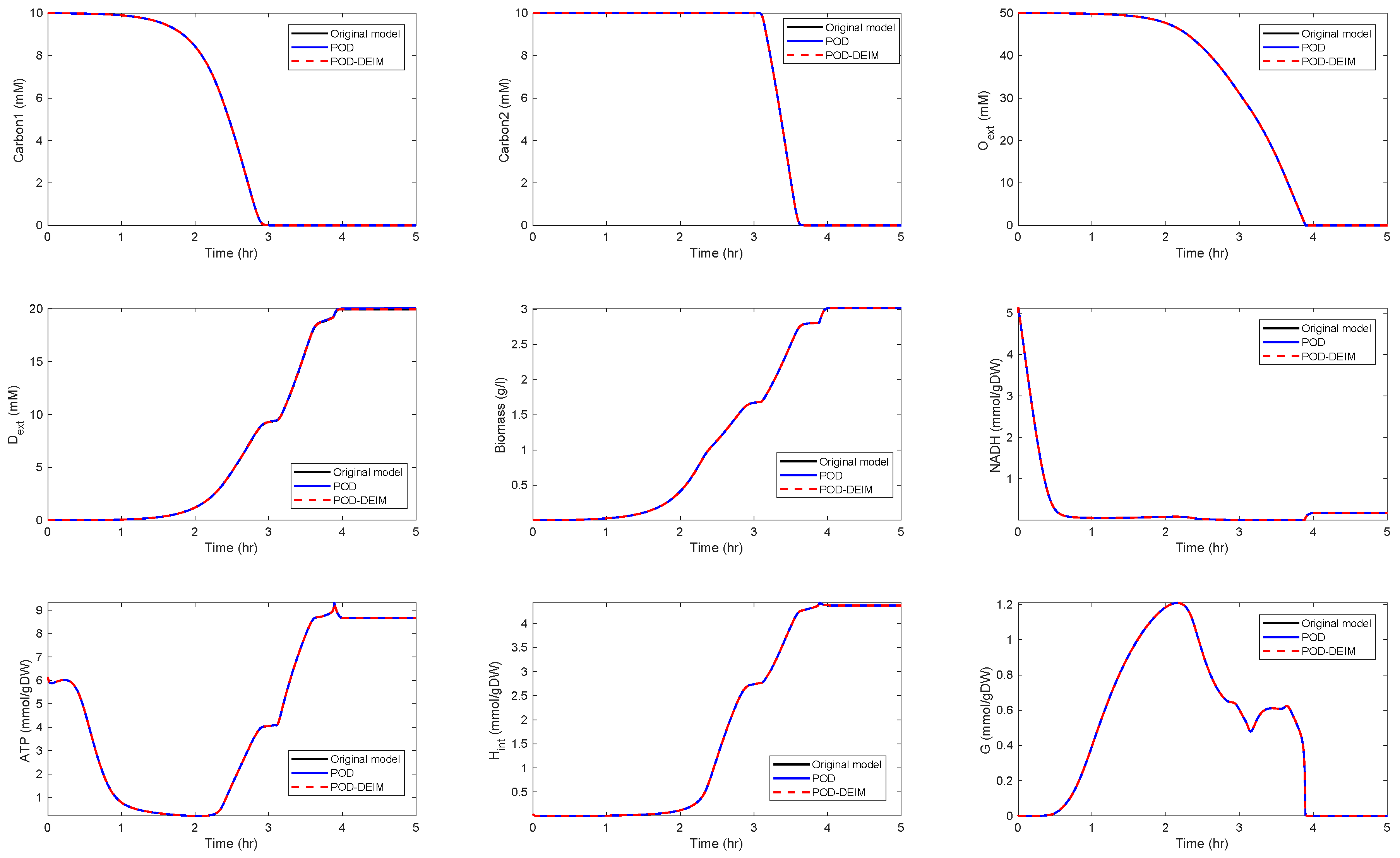
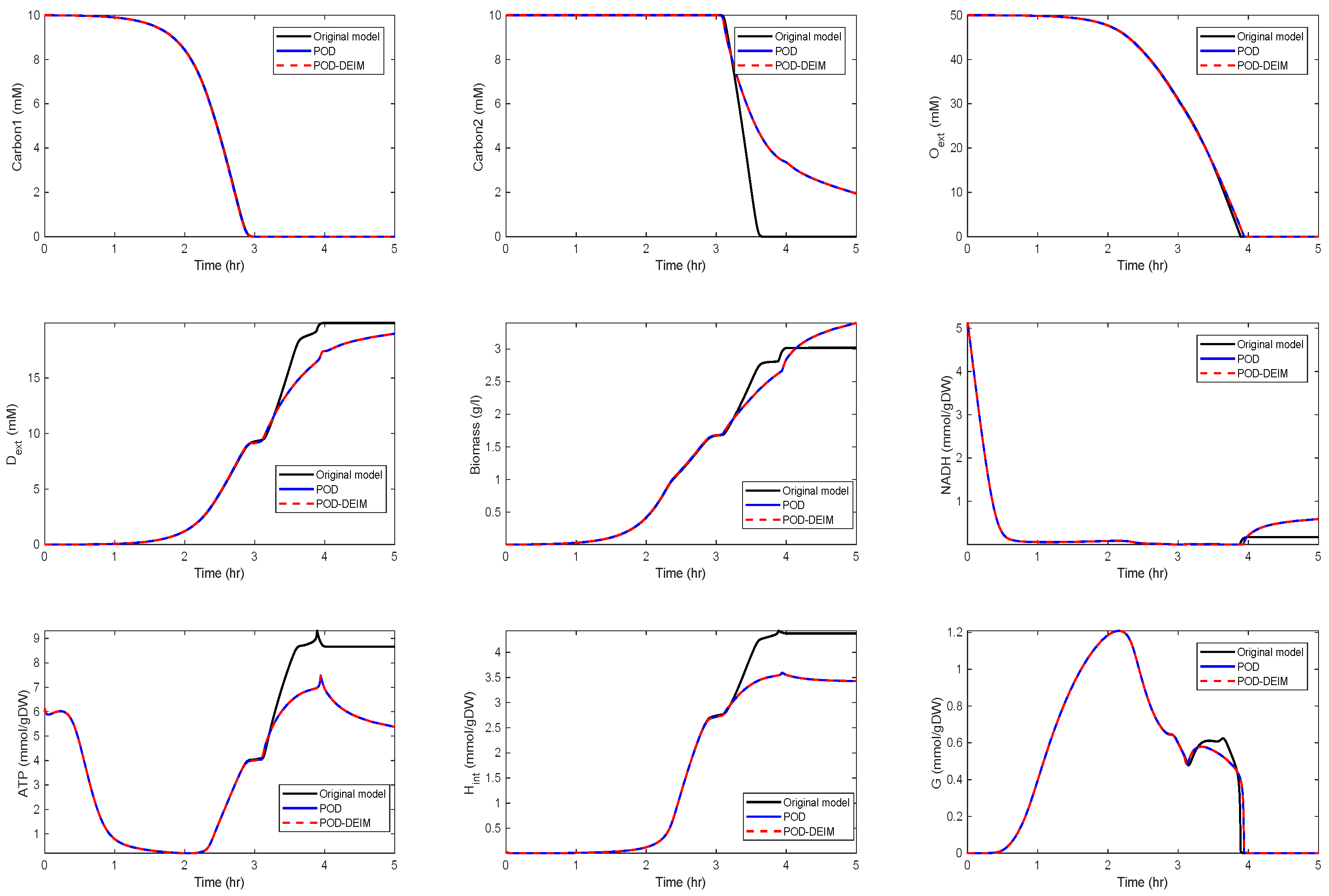
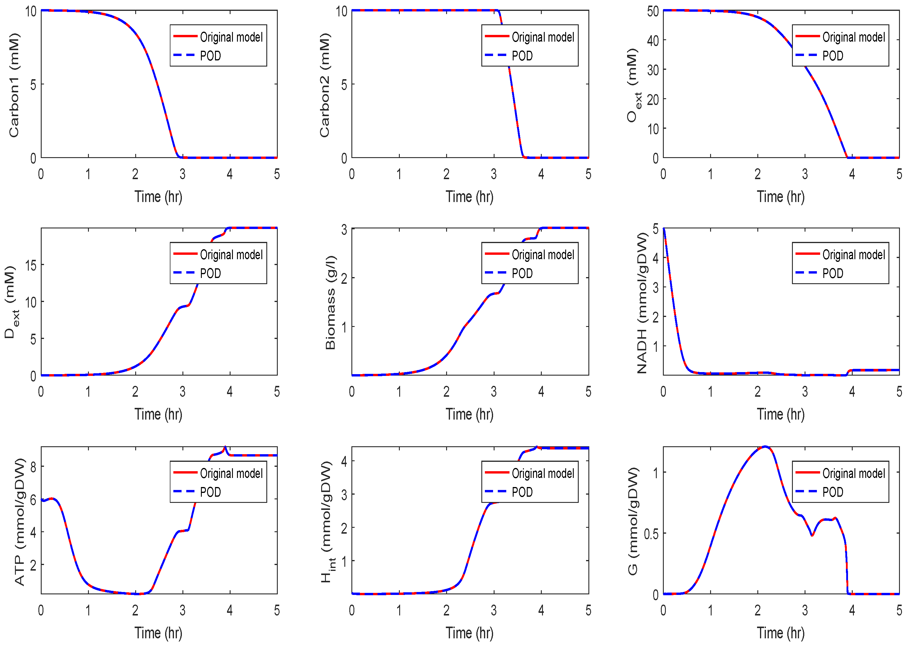
For , we could observe gradually decaying singular values with a strong decay for the smallest ones, indicating that neglecting these values would not result in any considerable loss of information in the reduced order model. A similar behavior could be observed for . The original model had a dimension of . We computed reduced order models of different dimensions, once using the POD approach and once using the POD-DEIM approach. In the first scenario, we used for both approaches. The simulation results of the reduced order system in comparison with the simulation results of the original system are depicted in Figure 3 for some selected components of the state vector. We could observe that the main features of the dynamical behavior of the original model states were preserved in both reduced order models.
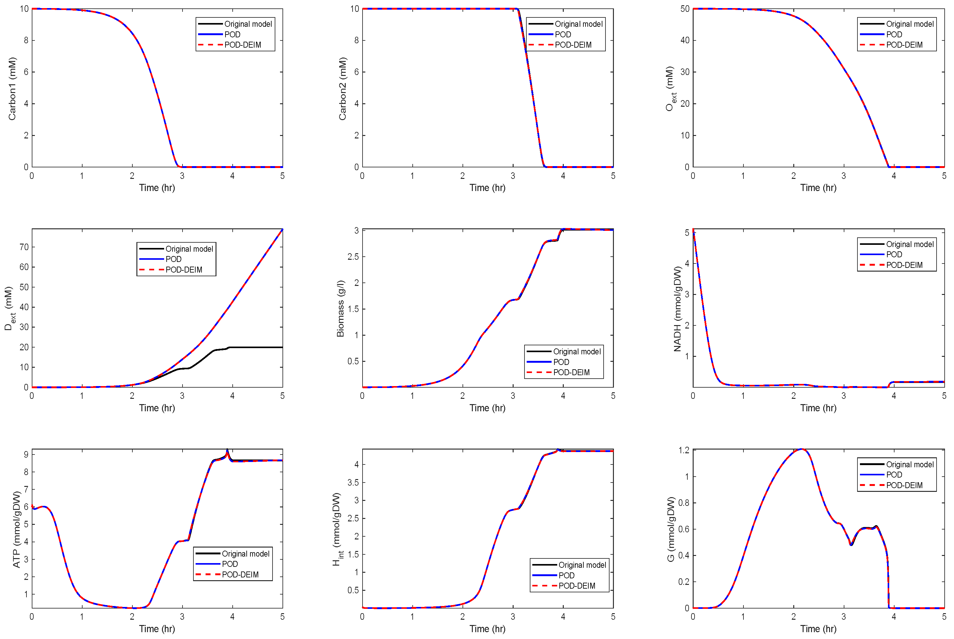
In a second scenario, we reduced the dimension to , . The results are depicted in Figure 4.
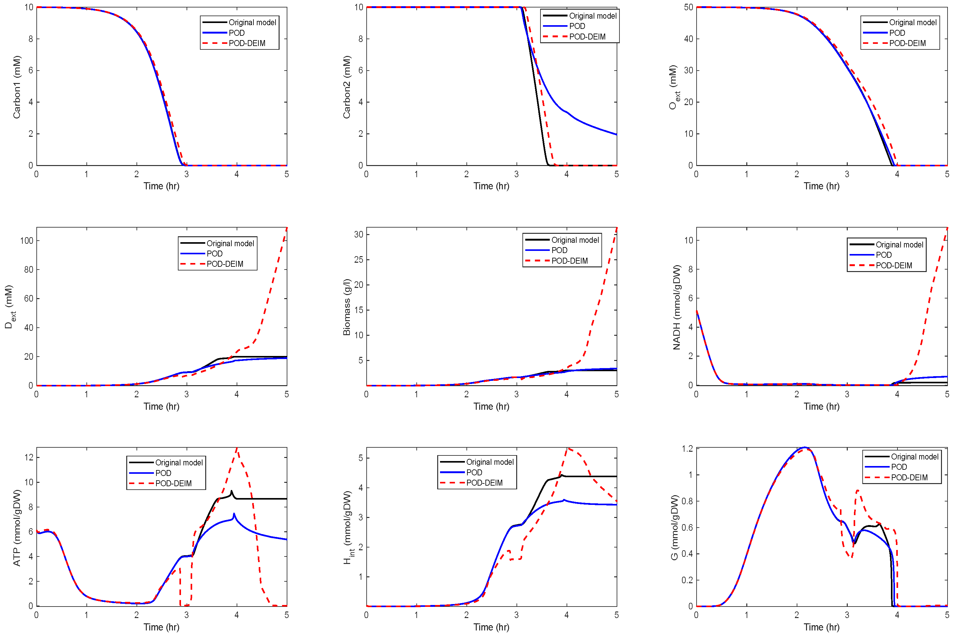
In a third scenario, we reduced the dimension to , . The results are depicted in Figure 5.
We can observe that some curves still matched well with the original model, while the solutions moved off, after hr in the second scenario and after hr in the third scenario. The behavior of , , and G still fit well for all reduced models.
Since biomass expresses the growth of the cell, it is an important component of the network that should also be preserved. We could observe that the reduced model preserved the biomass behavior quite well, such that we obtained approximately the same growth.
In the fourth scenario, we used and . The results are depicted in Figure 6.
We could observe that the trajectories of and still fit well, but deviations occurred for the other components. In particular, differences between the POD and the POD-DEIM models could be observed that suggested that information captured by the truncated SVDs was not sufficient to predict the original behavior. We also compared the time costs for the simulations; see Table 1. For evaluating the computing times, we used the MATLAB function timeit.
We could see that the calculation of the reduced order models required some additional computational effort, in particular the projections with and . If the reduced order model captured the features of the original model well, the computational effort for POD-DEIM model was about half of the effort for the POD model. This example was at a small scale, and the payoff in terms of computational time is shown in the later examples.
3.2. Kinetic Model of the Yeast Metabolic Network
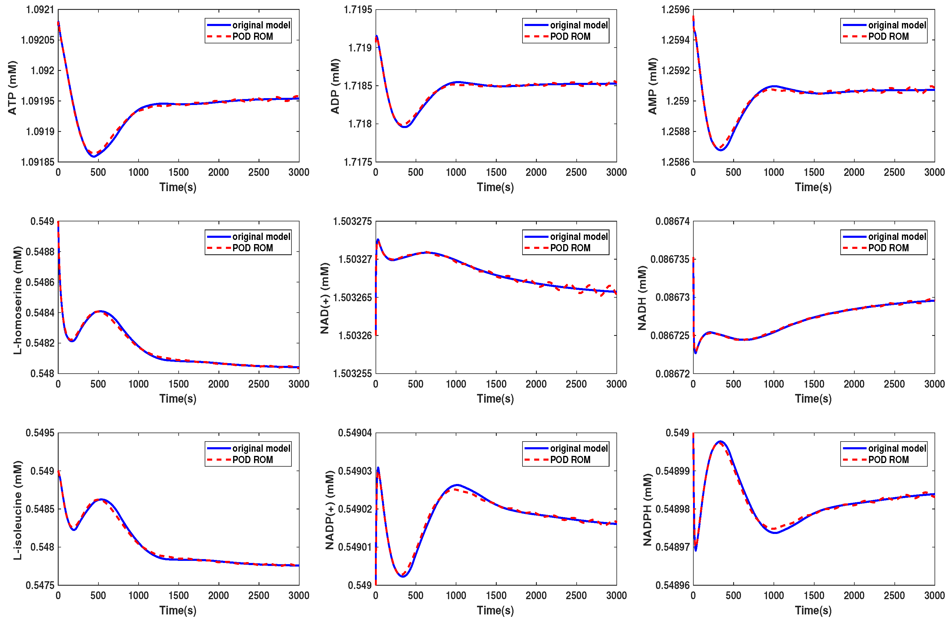
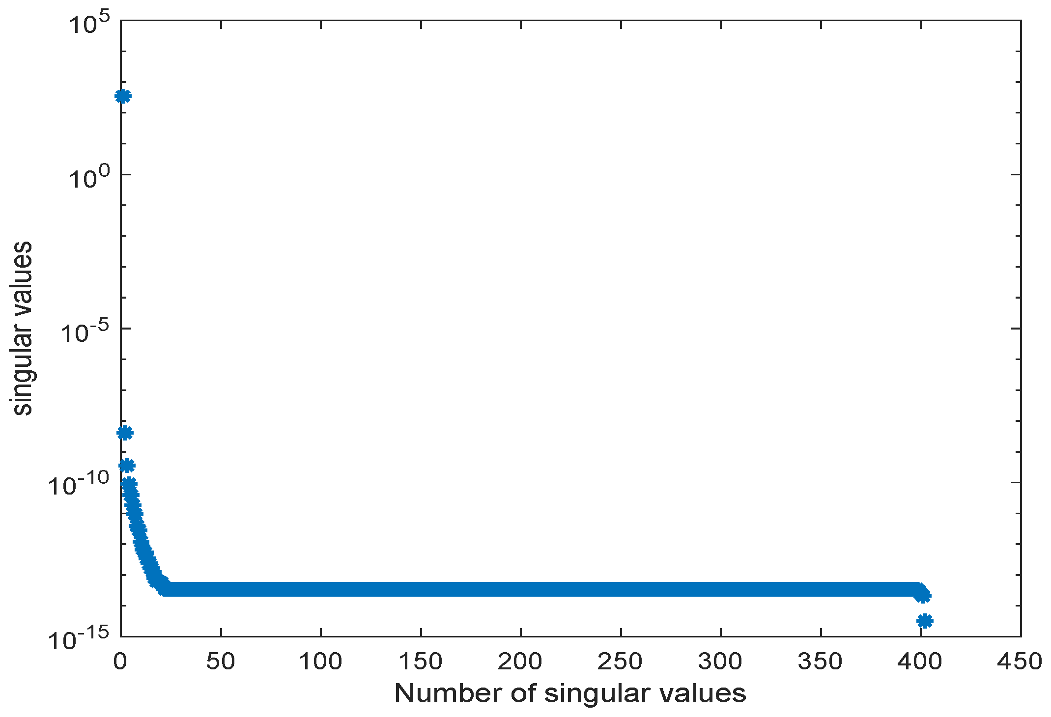
In [30], a workflow for converting metabolic reconstructions into large-scale kinetic models of yeast metabolism was developed. Its purpose was to take available datasets, perform a thorough analysis of the parameter constraints, and then, produce the kinetic model using large data integration. In this example, the generated kinetic model contained 281 metabolites. Here, we applied the order reduction method to the large-scale yeast model as described in [30]. The ODE model equations were taken from the BioModels database (http://identifiers.org/biomodels.db/BIOMD0000000496). Here, we used only some representative metabolites in order to compare the behavior of the original and the reduced order models. The snapshot matrix was obtained from a simulation of the ODE model over the time interval [0, 3000] s using the MATLAB solver ode23tb with the default setting and initial values taken from the database model. The behavior of the singular values of the snapshot matrix is depicted in Figure 7. We could observe a fast decay in the singular values with a large number of values of magnitude indicating that neglecting these values would not result in any considerable loss of information in the reduced order model.
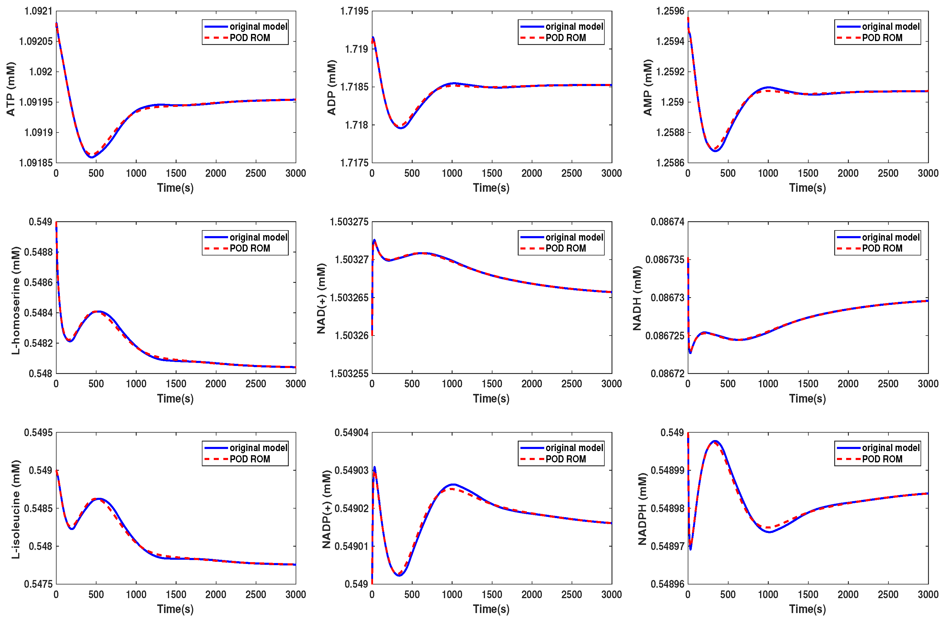
The original ODE system was of dimension , and we reduced it to (Scenario 1) and (Scenario 2). The results of the simulations are given in Figure 8 and Figure 9. A comparison of the computing times is given in Table 2.
We could see that in Scenario 1, the metabolites showed the same behavior in both models. We selected here the same metabolites as were presented in the Supplementary Information of [30]. In Scenario 2, the behavior of the metabolites was still well preserved, although we could see that some of the curves started to oscillate. The beginning oscillations suggested that the reduced order system was unstable, while the original system was stable. The problem of the instability of the reduced order model was addressed, e.g., in [34] or [35] and could be circumvented by taking additional measures. These oscillations increased if we further decreased the dimension of the reduced order model until the numerical simulation became unstable. The time cost of the simulation could be lowered by a factor of by approximately 3/4 in Scenario 1, whereas the oscillations led to a higher computational effort in Scenario 2.
For this example, we only applied the POD approach, since we could not gain any improvement in the computational efforts using the DEIM approach. The reason here was that the selection of the equation required in the DEIM method could not be achieved for the model equations provided by the BioModels database.
3.3. Kinetic Model of the E. coli Metabolic Network
A method for the generation of genome-scale kinetic models of the E. coli organism from reconstruction data was proposed in [31]. Building a kinetic model requires kinetic parameters, fluxes, and rate laws. In [31], a small kinetic model was used with the presence of experimental data, which was then extended using typical estimates in cases where experimental data were not available.
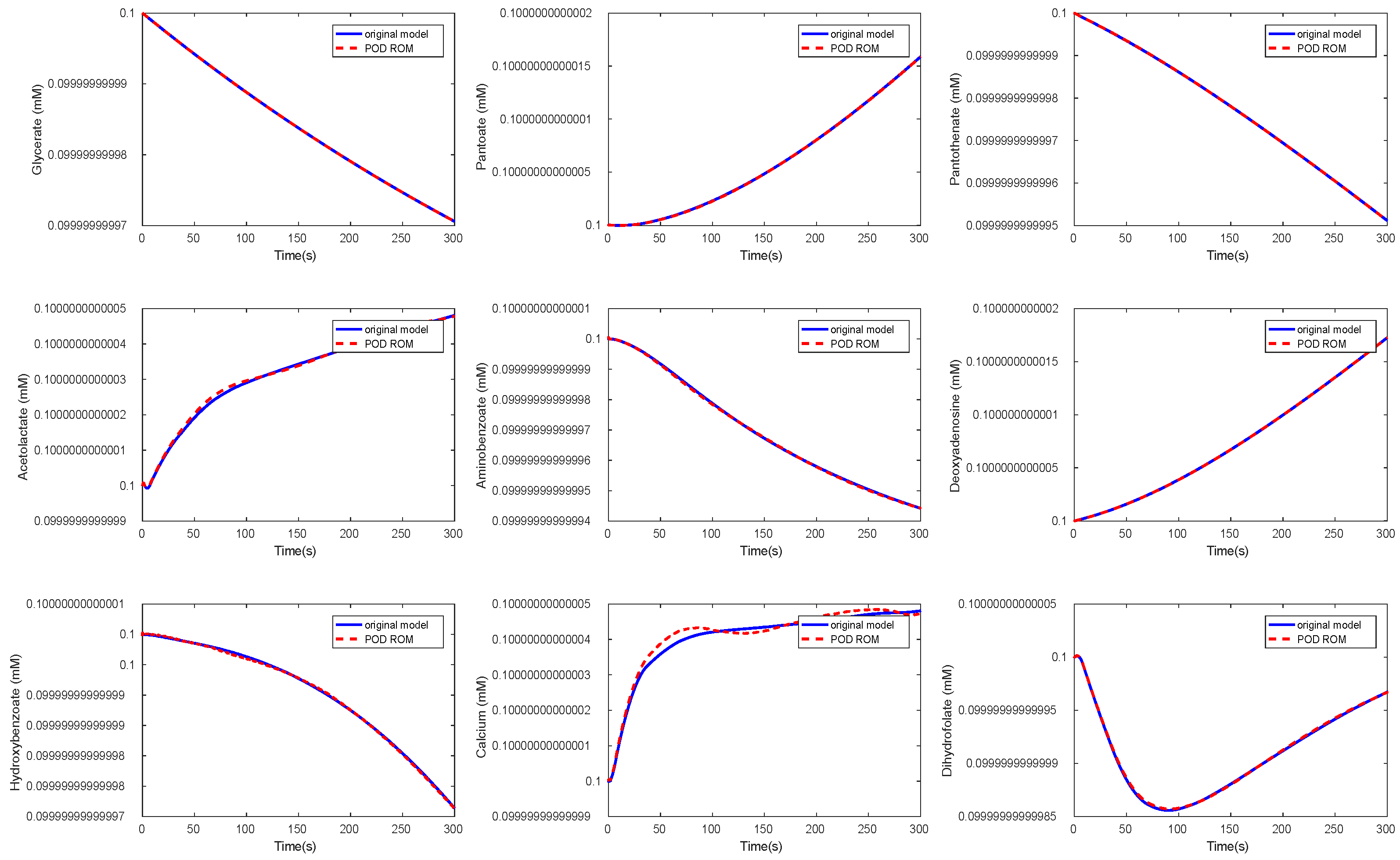
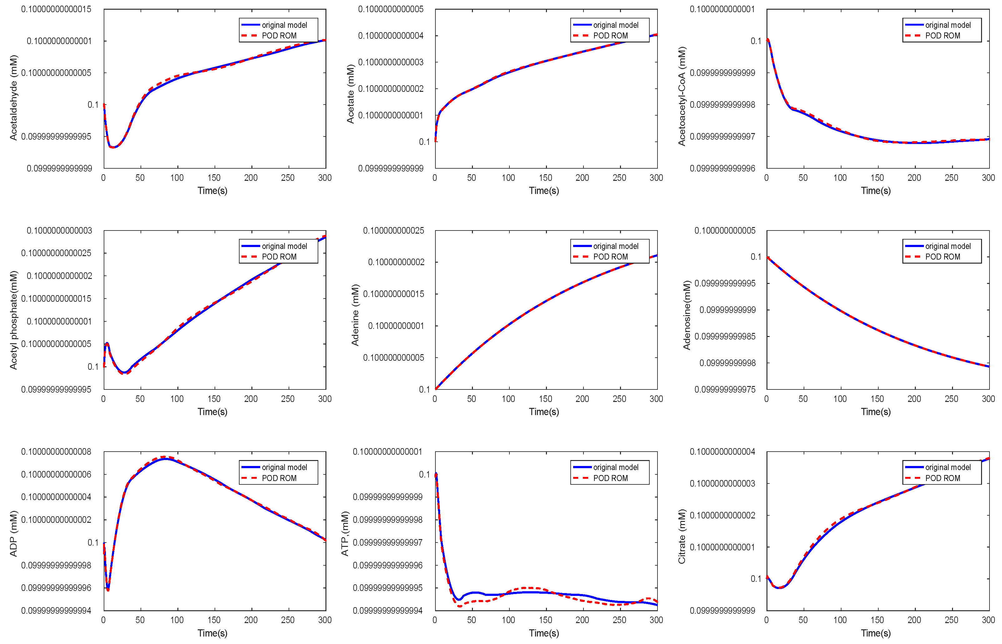
We applied the POD method to the generated kinetic model of E. coli as presented in [31] containing state variables, and we compared the original and reduced model for some of the metabolites’ behavior. The ODE model equations were taken from the BioModels database (http://identifiers.org/biomodels.db/BIOMD0000000469).
The snapshot matrix was obtained from a simulation of the ODE model over the time interval [0, 300] s using the MATLAB solver ode23tb setting and the initial values taken from the database model. The behavior of the singular values of the snapshot matrix is depicted in Figure 10.
Again, we could observe a fast decay in the singular values with a large number of values of magnitude indicating that neglecting these values would not result in any considerable loss of information in the reduced order model. The original ODE system was of dimension , and we reduced it to . The results of the simulations of some chosen metabolites are given in Figure 11 and Figure 12.
Here, we selected random metabolites for the comparison. We could observe that the metabolites showed the same behavior in both models. The time cost of the simulation in the reduced model could be lower by a factor of by approximately 1/7 compared to the original model, see Table 3.
From the previous discussions, we could conclude that the additional time cost required for the computation of the projection in the reduced order model in the POD approach was negligible for large-scale systems and was greatly exceeded by a gain in efficiency and computational speed. Naturally, the POD method was more effective and of more use in large-scale models.
4. POD for Kinetic Models With Different Initial Conditions
In this section, we study the POD method for a dynamical system with different initial conditions. In a kinetic system model, different initial conditions can be used to describe different scenarios or different modes of a biological system. We followed the same steps of the POD approach as in Section 2. At first, we computed the snapshot matrix by solving the system of ODEs (1) with the initial condition . Then, we computed another snapshot matrix with a different initial condition . We combined the two snapshot matrices in a snapshot matrix given in the following form:
Then, by applying the singular value decomposition, we obtained:
where and are unitary matrices with orthonormal columns. The term is a matrix with real, non-negative entries on the diagonal and zeros off the diagonal, and . By truncating the least dominant singular vectors and projecting the original system onto the lower-dimensional subspace, we obtain a reduced order model.
Application to the Kinetic Model of a Metabolic-Genetic Network
In the following, we apply the idea described above to the kinetic model of the metabolic-genetic network from [26] with model equations given in (A2) for different scenarios. The scenarios were the diauxic switch scenario and the aerobic/anaerobic-diauxie scenario, and both scenarios could be predicted using the kinetic model by prescribing specific initial values.
The model in the diauxic-switch scenario was already introduced in Section 3.1. We used the MATLAB function ode23s with tolerances and initial conditions
to compute a numerical solution of the ODE system (A2) with parameters in the time interval h using a non-equidistant output time-grid. This numerical solution yielded the snapshot matrix .
In the aerobic/anaerobic-diauxic scenario of transcriptional regulatory modeling, there was only one source of carbon (i.e., and ) and oxygen supplied to the culture. After some time, oxygen was removed [26]. We used the MATLAB function ode23s with tolerances and initial conditions
to compute a numerical solution of the ODE system (A2) with parameters in the time interval [0, 5] hr using a non-equidistant output time-grid. This numerical solution yielded the snapshot matrix .
We used the MATLAB function svd to calculate the singular value decompositions of . The singular values are depicted in Figure 13.
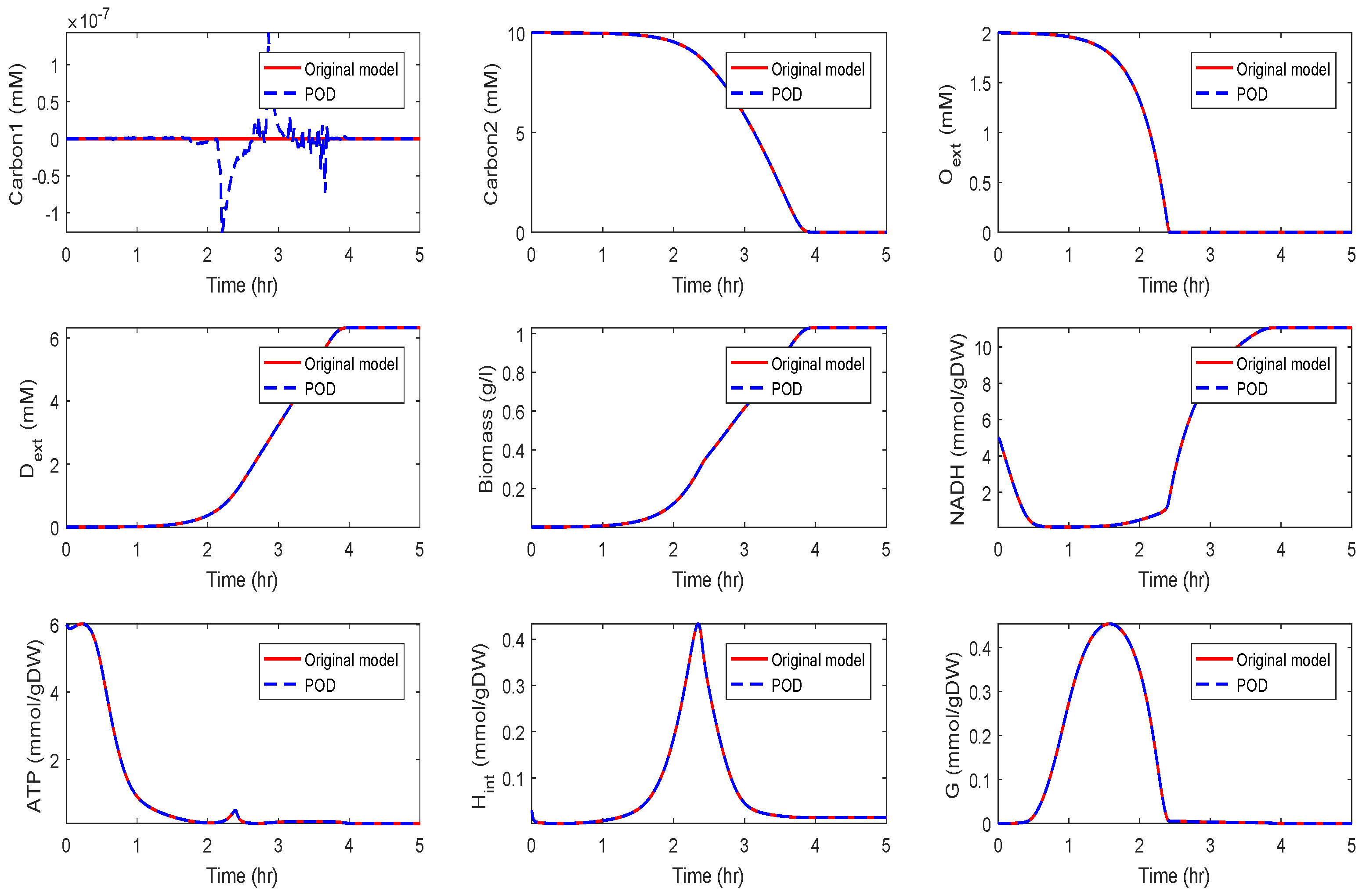
The original model had a dimension of . We computed a reduced order model of dimension using the POD approach. The results of a simulation of the reduced order system in comparison with the simulation results of the original system are depicted in Figure 14 and Figure 15 for the two different scenarios, diauxic switch and aerobic/anaerobic-diauxie, respectively.
We could observe that the main features of the dynamical behavior of the original model states were preserved for both scenarios using the same reduced order model. This was an important result, as it showed that as long as the snapshot matrix provided the essential information, a reduced order model had to be computed only once and could then be used to predict the dynamical behavior of the system for very different scenarios. The magnitude by which the system could be reduced depended on the decay of the singular values. Singular values of magnitude could be neglected, while singular values of order still contained important information. For large-scale networks as in Section 3.2 and Section 3.3, the difference in the dimension of the reduced and the original model could be assumed to be much larger.
5. Conclusions
In this paper, we discussed the model reduction for kinetic models of biological networks using the POD and the POD-DEIM approach. Since kinetic models of chemical networks can be very large, the possibility to obtain a reduced order model that replicates the desired dynamical behavior is of vital importance. We applied the model reduction techniques to several examples. It has to be noted that the computation of a reduced order model requires some additional computational effort. However, the computation of the snapshots and the SVD usually has to be computed only once (often, this is called the offline phase), while the simulations of the reduced order models are run several times, e.g., within an optimization process (in the so-called online phase). Thus, the effort for setting up a reduced order model will pay off if we can reduce a large-scale model to a much smaller dimension and run simulations of the reduced order model for a long time. Furthermore, the efficiency of the model order reduction strongly depends on the decay of the singular values of the snapshot matrix. How far the model can be reduced also depends on the application and on what components of the solution one is interested. In addition, we showed that the dynamical behavior of a biological network can be predicted for very different scenarios (diauxic switch and aerobic/anaerobic-diauxie) using the same reduced order model.
Author Contributions
N.A.E. wrote the first draft of the paper. All authors performed the numerical simulations, discussed the results, and contributed to the final version of the manuscript. All authors have read and agreed to the published version of the manuscript.
Funding
This research was supported by a PhD scholarship from the Egyptian Ministry of Higher Education (Cultural Affairs and Missions Sector) and the Deutsche Forschungsgemeinschaft (DFG, German Research Foundation) via the Research Training Groups (RTG 1772). L. Scholz was partially supported by the European Union’s Horizon 2020 research and innovation program under the Marie Skłodowska-Curie Grant Agreement No. 765374 and partially by the Berlin Mathematics Research Center MATH+.
Acknowledgments
We acknowledge support by the German Research Foundation and the Open Access Publication Fund of TU Berlin. We thank the anonymous reviewers for their helpful comments on the manuscript.
Conflicts of Interest
The authors declare no conflict of interest.
Appendix A
Appendix A.1. Derivation of Kinetic Model Equations
The simple metabolic-genetic network (see Figure 1) was presented in [26] via a discrete model of the regulatory flux balance analysis (rFBA). The rFBA model is based on steady-state assumptions and can be used to predict the time profile of the external metabolites and of the biomass concentration. Here, we derive a kinetic model of the metabolic-genetic network that mimics the discrete rFBA model, but allows describing the full dynamical behavior of the network.
The network has four regulatory rules that are expressed by Boolean logic in the rFBA model, defined in Table A1; see [26]. For instance, the presence of the metabolite will activate the regulatory protein , and the activation of (on) inhibits the transcriptional regulation (off).

Table A1.
Regulatory rules for the metabolic network Figure 1.
Table A1.
Regulatory rules for the metabolic network Figure 1.
| Regulatory Proteins | Transcriptional Regulation | ||
|---|---|---|---|
| IF () | IF NOT ( ) | ||
| IF () | IF NOT ( ) | ||
| IF () | IF NOT ( ) | ||
| IF Not () | IF NOT () | ||
In order to introduce a kinetic model for the network in Figure 1, the differential equations of a metabolic network can be given as follows:
where and are the vectors of external and internal metabolite concentrations, respectively, is the stoichiometric matrix [5] split into external and internal parts, v is the vector of reaction flux, and X denotes the biomass in the kinetic model. The factor describes the growth rate and is composed of the reaction fluxes , for all reactions , which produces biomass, multiplied by the corresponding yield coefficients . The yield coefficients are expressed as the mass of cells or product formed per unit mass of substrate consumed. Notice that in our model, . The regulatory proteins are expressed in our kinetic model by the Hill kinetics [36,37], yielding the following relations for the regulatory rules defined in Table A1:
where h is the Hill coefficient and , and are thresholds. We use the Michaelis–Menten kinetics [3] to model the reaction rates for the external metabolites, since the reactions are considered enzymatic reactions such that the enzyme active sites become saturated, yielding:
where , are the maximum transport rates and Michaelis–Menten constants, respectively. We use , , , and , all in mmol/(gDWh); see [26]. Furthermore, we use mass action kinetics [38] to model the reaction rates for internal metabolites, for the sake of simplicity and to reduce the number of kinetic parameters in comparison to the Michaelis–Menten kinetics, yielding:
where are the constant rates. Altogether, the differential equations to model the dynamical behavior of the simplified metabolic-genetic network are given by:
Appendix A.2. Model Fitting
The kinetic model we introduced contains unknown parameters (constant rates). In order to find the parameter values, we performed a model fitting process to best fit to the given datasets, i.e., the simulation results of the rFBA model and in particular the biomass and external metabolite concentrations over discrete time steps; see [26]. For the model fitting, the DataToDynamics (D2D) toolbox was used that is based on a maximum likelihood estimation [39,40]. We assumed that the kinetic model Equation (A1) was given by an ODE:
where denotes the concentration vector and is a vector of parameters (the kinetic parameters and the thresholds in the Hill functions). In order to calibrate the kinetic model (A3) to a given dataset, the dynamic states x are linked to measurements via:
where y is the simulation result of rFBA of external metabolites and biomass at some time point and g is the observation function involving the parameter . In our model, the observation function g is the dynamical state of external metabolites and biomass. The measurement noise is assumed to be normally distributed with mean 0 and variance such that ; see [39].
The model was fitted to two different datasets for the diauxic switch and aerobic/anaerobic-diauxie scenarios of the cell, which were mentioned in [26], with the initial conditions of external metabolites and , respectively. The estimated parameters are given in Table A2.
Table A2.
The set of all parameters of the model that are estimated of two datasets of the diauxic switch and aerobic/anaerobic-diauxie scenarios using the D2D toolbox.
Table A2.
The set of all parameters of the model that are estimated of two datasets of the diauxic switch and aerobic/anaerobic-diauxie scenarios using the D2D toolbox.
| Constant Rates | Value | Unit | |
|---|---|---|---|
| mM | estimated | ||
| mM | estimated | ||
| mM | estimated | ||
| mM | estimated | ||
| mmol/gDW | estimated | ||
| mmol/gDW | estimated | ||
| 41 | mM | estimated | |
| 980 | mmol3/gDW3 · h−1 | estimated | |
| 1000 | mmol2/gDW2 · h−1 | estimated | |
| 300 | mmol/gDW · h−1 | estimated | |
| 140 | mmol3/gDW3 · h−1 | estimated | |
| 23 | mmol/gDW · h−1 | estimated | |
| 25 | mmol/gDW · h−1 | estimated | |
| mmol/gDW· h−1 | estimated | ||
| 1000 | mmol/gDW· h−1 | estimated | |
| 13 | mmol/gDW· h−1 | estimated | |
| mmol2/gDW2· h−1 | estimated | ||
| 150 | mmol3/gDW3 · h−1 | estimated | |
| mmol/gDW· h−1 | estimated | ||
| 170 | mmol2/gDW2 · h−1 | estimated | |
| mM | estimated | ||
| mmol/gDW | estimated | ||
| mM | estimated | ||
| 290 | mmol/gDW | estimated | |
| 1 | gDW/mmol | assumed |
References
- Gerdtzen, Z.P.; Daoutidis, P.; Hu, W.-S. Non-linear reduction for kinetic models of metabolic reaction networks. Metab. Eng. 2004, 6, 140–154. [Google Scholar] [CrossRef]
- Briggs, G.E.; Sanderson Haldane, J.B. A note on the kinetics of enzyme action. Biochem. J. 1925, 19, 338. [Google Scholar] [CrossRef] [Green Version]
- Michaelis, L.; Menten, M.L. Die Kinetik der Invertinwirkung. Biochem Z 1913, 49, 333–369. [Google Scholar]
- Nelson, D.L.; Cox, M.M. Hormonal regulation of food metabolism. In Lehninger Principles of Biochemistry, 4th ed.; WH Freeman: New York, NY, USA, 2005; pp. 881–992. [Google Scholar]
- Sontag, E.D. Lecture Notes on Mathematical Systems Biology; Northeastern University: Boston, MA, USA, 2005. [Google Scholar]
- Snowden, T.J.; van der Graaf, P.H.; Tindall, M.J. Methods of model reduction for large-scale biological systems: A survey of current methods and trends. Bull. Math. Biol. 2017, 79, 1449–1486. [Google Scholar] [CrossRef] [Green Version]
- Costa, R.S.; Rocha, I.; Ferreira, E.C. Model Reduction Based on Dynamic Sensitivity Analysis: A Systems Biology Case of Study. 2008. Available online: http://citeseerx.ist.psu.edu/viewdoc/summary?doi=10.1.1.619.3225 (accessed on 8 May 2020).
- Zi, Z. Sensitivity analysis approaches applied to systems biology models. IET Syst. Biol. 2011, 5, 336–346. [Google Scholar] [CrossRef]
- Kuo, J.C.W.; Wei, J. Lumping analysis in monomolecular reaction systems. analysis of approximately lumpable system. Ind. Eng. Chem. Fund. 1969, 8, 124–133. [Google Scholar] [CrossRef]
- Wei, J.; Kuo, J.C.W. Lumping analysis in monomolecular reaction systems. analysis of the exactly lumpable system. Ind. Eng. Chem. Fund. 1969, 8, 114–123. [Google Scholar] [CrossRef]
- Okeke, B.E. Lumping Methods for Model Reduction. Ph.D. Thesis, University of Lethbridge, Lethbridge, AB, Canada, 2013. [Google Scholar]
- Pepiot-Desjardins, P.; Pitsch, H. An automatic chemical lumping method for the reduction of large chemical kinetic mechanisms. Combust. Theory Model. 2008, 12, 1089–1108. [Google Scholar] [CrossRef]
- Okino, M.S.; Mavrovouniotis, M.L. Simplification of mathematical models of chemical reaction systems. Chem. Rev. 1998, 98, 391–408. [Google Scholar] [CrossRef] [PubMed]
- Flach, E.; Schnell, S. Use and abuse of the quasi-steady-state approximation. IEE Proc.-Syst. Biol. 2006, 153, 187–191. [Google Scholar] [CrossRef] [Green Version]
- Khalil, H.K.; Grizzle, J.W. Nonlinear Systems; Prentice Hall: Upper Saddle River, NJ, USA, 2002; p. 3. [Google Scholar]
- Tikhonov, A.N. Systems of differential equations containing small parameters in the derivatives. Matematicheskii Sbornik 1952, 73, 575–586. [Google Scholar]
- Kuntz, J.; Oyarzún, D.; Stan, G.-B. Model reduction of genetic-metabolic networks via time scale separation. In A Systems Theoretic Approach to Systems and Synthetic Biology I: Models and System Characterizations; Springer: Berlin, Germany, 2014; pp. 181–210. [Google Scholar]
- Duan, Z.; Cruz Bournazou, M.N.; Kravaris, C. Dynamic model reduction for two-stage anaerobic digestion processes. Chem. Eng. J. 2017, 327, 1102–1116. [Google Scholar] [CrossRef]
- Belgacem, I.; Casagranda, S.; Grac, E.; Ropers, D.; Gouzé, J.-L. Reduction and stability analysis of a transcription–translation model of RNA polymerase. Bull. Math. Biol. 2018, 80, 294–318. [Google Scholar] [CrossRef] [PubMed] [Green Version]
- Karhunen, K. Über Lineare Methoden in der Wahrscheinlichkeitsrechnung. Sana 1947, 37. [Google Scholar]
- Loeve, M. Elementary probability theory. In Probability Theory I; Springer: Berlin, Germany, 1977; pp. 1–52. [Google Scholar]
- Brunton, S.L.; Kutz, J.N. Data-Driven Science and Engineering: Machine Learning, Dynamical Systems, and Control; Cambridge University Press: Cambridge, UK, 2019. [Google Scholar]
- Golub, G.H.; Reinsch, C. Singular value decomposition and least squares solutions. In Linear Algebra; Springer: Berlin, Germany, 1971; pp. 134–151. [Google Scholar]
- Strang, G. Introduction to Linear Algebra; Wellesley-Cambridge Press: Wellesley, MA, USA, 1993; Volume 3. [Google Scholar]
- Chaturantabut, S.; Sorensen, D. Nonlinear model reduction via discrete empirical interpolation. SIAM J. Sci. Comput. 2010, 32, 2737–2764. [Google Scholar] [CrossRef]
- Covert, M.W.; Schilling, C.H.; Palsson, B. Regulation of gene expression in flux balance models of metabolism. J. Theor. Biol. 2001, 213, 73–88. [Google Scholar] [CrossRef] [Green Version]
- Beattieand, C.; Gugercin, S.; Mehrmann, V. Model reduction for systems with inhomogeneous initial conditions. Syst. Control Lett. 2017, 99, 99–166. [Google Scholar] [CrossRef] [Green Version]
- Chaturantabut, S.; Sorensen, D. A state space error estimate for POD-DEIM nonlinear model reduction. SIAM J. Numer. Anal. 2012, 50, 46–63. [Google Scholar] [CrossRef]
- Afanasiev, K.; Hinze, M. Adaptive control of a wake flow using proper orthogonal decomposition1. Lect. Notes Pure Appl. Math. 2001, 1, 216. [Google Scholar] [CrossRef]
- Stanford, N.J.; Lubitz, T.; Smallbone, K.; Klipp, E.; Mendes, P.; Liebermeister, W. Systematic Construction of Kinetic Models from Genome-Scale Metabolic Networks. PLoS ONE 2013, 8, e79195. [Google Scholar] [CrossRef] [Green Version]
- Smallbone, K.; Mendes, P. Large-scale metabolic models: From reconstruction to differential equations. Ind. Biotechnol. 2013, 9, 179–184. [Google Scholar] [CrossRef] [Green Version]
- Badreddine, A.-A.; Henrik, P. Simulation of switching phenomena in biological systems. In Biochemical Engineering for 2001; Springer: Berlin, Germany, 1992; pp. 701–704. [Google Scholar]
- Kremling, A.; Kremling, S.; Bettenbrock, K. Catabolite repression in escherichia coli—a comparison of modelling approaches. FEBS J. 2009, 276, 594–602. [Google Scholar] [CrossRef] [PubMed] [Green Version]
- Rosa, C.S.; Boris, L.; Rudy, E. Stability Preservation in Projection-based Model Order Reduction of Large Scale Systems. Eur. J. Control 2012, 18, 122–132. [Google Scholar]
- Roland, P. Stability preservation in Galerkin-type projection-based model order reduction. arXiv 2017, arXiv:1711.02912. [Google Scholar]
- Gesztelyi, R.; Zsuga, J.; Kemeny-Beke, A.; Varga, B.; Juhasz, B.; Tosaki, A. The Hill Equation and the Origin of Quantitative Pharmacology; Springer: Berlin, Germany, 2012; Volume 66, pp. 427–438. [Google Scholar]
- Hill, A.V. The possible effects of the aggregation of the molecules of hæmoglobin on its dissociation curves. J. Physiol. 1910, 40, i–vii. [Google Scholar]
- Guldberg, C.M.; Waage, P. Etudes sur Les Affinités Chimiques; Brøgger & Christie: Oslo, Norway, 1867. [Google Scholar]
- Raue, A.; Steiert, B.; Schelker, M.; Kreutz, C.; Maiwald, T.; Hass, H.; Vanlier, J.; Tönsing, C.; Adlung, L.; Engesser, R.; et al. Data2Dynamics: A modeling environment tailored to parameter estimation in dynamical systems. Bioinformatics 2015, 31, 3558–3560. [Google Scholar] [CrossRef] [Green Version]
- Raue, A.; Schilling, M.; Bachmann, J.; Matteson, A.; Schelke, M.; Kaschek, D.; Hug, S.; Kreutz, C.; Harms, B.D.; Theis, F.J.; et al. Lessons Learned from Quantitative Dynamical Modeling in Systems Biology. PLoS ONE 2013, 8, 1932–6203. [Google Scholar] [CrossRef]
Figure 1.
A network of chemical reactions of the core carbon metabolic network [26].
Figure 1.
A network of chemical reactions of the core carbon metabolic network [26].

Figure 2.
Singular values of snapshot matrix (left) and nonlinear snapshot matrix (right) for the simple metabolic-genetic network example of [26].
Figure 2.
Singular values of snapshot matrix (left) and nonlinear snapshot matrix (right) for the simple metabolic-genetic network example of [26].

Figure 3.
Comparison of some of the model components in the original model and the reduced order models (proper orthogonal decomposition (POD) and POD-discrete empirical interpolation method (DEIM)) of dimension , .
Figure 3.
Comparison of some of the model components in the original model and the reduced order models (proper orthogonal decomposition (POD) and POD-discrete empirical interpolation method (DEIM)) of dimension , .

Figure 4.
Comparison of some of the model components in the original model and the reduced order models (POD and POD-DEIM) of dimension , .
Figure 4.
Comparison of some of the model components in the original model and the reduced order models (POD and POD-DEIM) of dimension , .

Figure 5.
Comparison of some of the model components in the original model and the reduced order models (POD and POD-DEIM) of dimension , .
Figure 5.
Comparison of some of the model components in the original model and the reduced order models (POD and POD-DEIM) of dimension , .

Figure 6.
Comparison of some of the model components in the original model and the reduced order models (POD and POD-DEIM) of dimension , .
Figure 6.
Comparison of some of the model components in the original model and the reduced order models (POD and POD-DEIM) of dimension , .

Figure 7.
Singular values of snapshot matrix .

Figure 8.
Comparison of the behavior of some metabolites in the yeast model for the original and the POD reduced model (Scenario 1).
Figure 8.
Comparison of the behavior of some metabolites in the yeast model for the original and the POD reduced model (Scenario 1).

Figure 9.
Comparison of the behavior of some metabolites in the yeast model for the original and the POD reduced model (Scenario 2).
Figure 9.
Comparison of the behavior of some metabolites in the yeast model for the original and the POD reduced model (Scenario 2).

Figure 10.
Singular values of snapshot matrix for the kinetic model of the E. coli metabolic network of [31].
Figure 10.
Singular values of snapshot matrix for the kinetic model of the E. coli metabolic network of [31].

Figure 11.
Comparison of the behavior of some metabolites in the yeast model for the original and the POD reduced model.
Figure 11.
Comparison of the behavior of some metabolites in the yeast model for the original and the POD reduced model.

Figure 12.
Comparison of the behavior of some metabolites in the yeast model for the original and the POD reduced model.
Figure 12.
Comparison of the behavior of some metabolites in the yeast model for the original and the POD reduced model.

Figure 13.
Singular values of snapshot matrix for the simple metabolic-genetic network example of [26].
Figure 13.
Singular values of snapshot matrix for the simple metabolic-genetic network example of [26].

Figure 14.
Comparison of the behavior of some metabolites in the diauxic switch scenario for the original and the POD reduced model.
Figure 14.
Comparison of the behavior of some metabolites in the diauxic switch scenario for the original and the POD reduced model.

Figure 15.
Comparison of the behavior of some metabolites in the aerobic/anaerobic-diauxie scenario for the original and the POD reduced model.
Figure 15.
Comparison of the behavior of some metabolites in the aerobic/anaerobic-diauxie scenario for the original and the POD reduced model.

Table 1.
Comparison of the computing times for the four different scenarios.
| Original Model | POD ROM | POD-DEIM ROM | |
|---|---|---|---|
| Scenario 1 (, ) | 0.3 s | 1.4 s | 0.7 s |
| Scenario 2 (, ) | 0.3 s | 1.4 s | 0.6 s |
| Scenario 3 (, ) | 0.3 s | 1.9 s | 0.9 s |
| Scenario 4 (, ) | 0.3 s | 1.9 s | 0.9 s |
Table 2.
Comparison of the computing times for the two different scenarios.
| Original Model | POD ROM | |
|---|---|---|
| Scenario 1 () | 0.28 s | 0.20 s |
| Scenario 2 () | 0.28 s | 0.46 s |
Table 3.
Computing times for the POD method.
| Original Model | POD ROM | |
|---|---|---|
| Scenario () | 0.10 s | 0.014 s |
© 2020 by the authors. Licensee MDPI, Basel, Switzerland. This article is an open access article distributed under the terms and conditions of the Creative Commons Attribution (CC BY) license (http://creativecommons.org/licenses/by/4.0/).
Share and Cite
MDPI and ACS Style
Ali Eshtewy, N.; Scholz, L. Model Reduction for Kinetic Models of Biological Systems. Symmetry 2020, 12, 863. https://0-doi-org.brum.beds.ac.uk/10.3390/sym12050863
AMA Style
Ali Eshtewy N, Scholz L. Model Reduction for Kinetic Models of Biological Systems. Symmetry. 2020; 12(5):863. https://0-doi-org.brum.beds.ac.uk/10.3390/sym12050863
Chicago/Turabian StyleAli Eshtewy, Neveen, and Lena Scholz. 2020. "Model Reduction for Kinetic Models of Biological Systems" Symmetry 12, no. 5: 863. https://0-doi-org.brum.beds.ac.uk/10.3390/sym12050863
Note that from the first issue of 2016, this journal uses article numbers instead of page numbers. See further details here.