Multi-Classifier Decision-Level Fusion Classification of Workpiece Surface Defects Based on a Convolutional Neural Network

Abstract

Various defects are formed on the workpiece surface during the production process. Workpiece surface defects are classified according to various characteristics, which includes a bumped surface, scratched surface and pit surface. Suppliers analyze the cause of workpiece surface defects through the defect types and thus determines the subsequent processing. Therefore, the correct classification is essential regarding workpiece surface defects. In this paper, a multi-classifier decision-level fusion classification model for workpiece surface defects based on a convolutional neural network (CNN) was proposed. In the proposed model, the histogram of oriented gradient (HOG) was used to extract the features of the second fully connected layer of the CNN, and the features of the HOG were further extracted by using the local binary patterns (LBP), which was called the HOG–LBP feature extraction. Finally, this paper designed a symmetry ensemble classifier, which was used to classify the features of the last fully connected layer of the CNN and the features of the HOG–LBP. The comprehensive decision was made by fusing the classification results of the symmetry structure channels. The experiments were carried out, and the results showed that the proposed model could improve the accuracy of the workpiece surface defect classification.

1. Introduction

Workpiece surface defects are one of the main factors that lower the quality of the workpiece. Some defects not only affect subsequent production, but also affect the corrosion resistance and wear resistance of the final product. However, due to technical and cost constraints, manpower is still used to detect surface defects in most companies. Magnifying glasses and auxiliary tools are often used to detect subtle surface defects by manual visual inspection. However, this method is inefficient and poorly flexible, the labor intensity is high and it is susceptible to subjective factors, which leads to inaccurate detection results and is unable to meet the requirement of online inspection. Machine vision detection has the advantages of a high degree of automation, high recognition rate and non-contact measurement. Therefore, it is a development trend to detect surface defects. A CCD camera is used to capture the images of the workpiece surface defects under special illumination. Some defect recognition algorithms are used to process these images, and surface defects are detected and classified [1,2,3].

Defect classification is the most important part of the surface defect detection system [4,5,6]. Classification results can be used to grade workpieces and improve manufacturing techniques. In recent years, many researchers have been studying the classification of workpiece surface defects. A weld defect detection based on support vector machines (SVM) was proposed; the trained SVM was used to distinguish real defects from potential defects [7], but there was a problem in that the degree of feature extraction was not high. The construction of a multi-core SVM classifier was designed and multi-core learning was converted into second-order cone programming; the new model was superior to the traditional SVM for surface defect images [8]. A method based on a decision tree was proposed to detect defects [9]; however, the method had low feature extraction and a low detection efficiency. A multi-stage convolutional neural network (CNN) and an ensemble CNN with different structures were proposed to accomplish the defect classification tasks automatically [10].

Effective feature extraction can improve the classification effect of the algorithm. Twelve typical features were extracted, and the defect types were differentiated by using two well-known classifiers: fuzzy k-nearest neighbor and multi-layer perceptron neural networks classifiers [11]. A method based on scale invariant feature transform (SIFT) and SVM was proposed to detect steel surface defects [12]. The SIFT was used for defect region detection and to extract features, and the SVM was used for classification. The results showed that the key to a successful classification was to choose the appropriate method for accurate feature extraction. To avoid the dimensional disaster, the classification effect was improved by using an effective feature extraction algorithm with an appropriate classifier [13]. However, the abovementioned feature extraction method requires relevant knowledge of professional surface defect image processing.

To date, many efforts have been focused on the design of feature extraction algorithms because traditional classifiers cannot automatically extract representative features from the original image. At present, deep learning is used for feature learning for image recognition and classification [14,15,16]. A CNN allows deep learning to learn more data features [17], and can achieve finding the important parameters by constructing multi-layer structures like human brains, which can remove many unimportant parameters to achieve better learning results. Therefore, additional step of feature extraction on the original image is unnecessary. The feature size can be synchronously reduced in the feature learning process of a CNN; thus, it can reduce the dimension and retain the feature. A CNN can easily adapt to the problem of image classification; if the number of samples is insufficient and the classification efficiency is low, it is effective to use the CNN with transfer learning to make the pre-trained deep network suitable for classification problems [18,19,20]. Moreover, CNNs have been successfully applied for almost all classification and detection tasks in image and speech analysis [21,22].

Traditional feature extraction methods are more reliable for capturing local image features, such as the gray-level co-occurrence matrix (GLCM), local binary pattern (LBP) analysis and histogram of oriented gradient (HOG), which are widely used in the field of classification detection [23,24,25]. When the surface defect features are not obvious, traditional extraction feature methods contain many unrelated certain features, and the features are not effectively selected. Therefore, a model is proposed in this paper that uses the HOG–LBP to assist the CNN to extract features, and the symmetry ensemble classifier output results is fitted to the posterior probability of the target category. The decision weights of each classifier are obtained from the correct classification rate, which is obtained and normalized by each classifier. Decision weights are used to perform decision-level fusion, and the traditional feature extraction method and the advantages of the CNN feature extraction method are effectively combined. Some experiments were carried out and the results indicated that the proposed model has high robustness and accuracy.

The rest of this paper is organized as follows: Section 2 describes the proposed model in detail; Section 3 presents the experimental results and discussions; and Section 4 draws some conclusions.

2. The Proposed Classification Model

2.1. CNN Feature Extraction

Most in-depth and broader CNN models have demonstrated their effectiveness in defect classification [26,27]. However, it is not appropriate to apply them directly to the classification task of workpiece surface defects; this is because the particularity of the surface defects, such as small and inconspicuous surface defect features, are not considered, and existing workpiece surfaces defect data is too small to train this deeper and wider model. The Alexnet model is used to extract features in the proposed method, which is a shallow CNN model, and the transfer learning can be used to compensate the problem of existing workpiece surface defect data shortage [28]. As shown in

Table 1. The parameters of the adopted convolutional neural network (CNN).

Layer	Layer Type	Convolution Kernel/Pooling Areas	Step Size	Graphs	Size
C1	convolutional layer	11 × 11	4	96	55 × 55
S2	pooling layer	3 × 3	2	96	27 × 27
C3	convolutional layer	5 × 5	1	256	27 × 27
S4	pooling layer	3 × 3	2	256	13 × 13
C5	convolutional layer	3 × 3	1	384	13 × 13
C6	convolutional layer	3 × 3	1	384	13 × 13
C7	convolutional layer	3 × 3	1	256	13 × 13
S8	pooling layer	3 × 3	2	256	6 × 6
F9	fully connected layer	−	−	4096	1 × 1
F10	fully connected layer	−	−	4096	1 × 1
F11	fully connected layer	−	−	4	1 × 1

, the Alexnet model consists of 5 convolution layers (i.e., C1, C3, C5, C6, C7), 3 pooling layers (i.e., S2, S4, S8) and 3 fully connected layers (i.e., F9, F10, F11).

In the input layer, an input image with a size of 227 × 227 × 3 was used. The convolutional layer with an 11 × 11 convolution kernel was preformed, and the pooling layer with a size of 3 × 3 was performed. The convolution and pooling operations were continuously performed, and the fully connected layer and the final classifier classification were calculated.

2.2. HOG–LBP Feature Extraction

2.2.1. Histogram of Oriented Gradients: HOG Feature

Dalal and Triggs proposed a representation of the HOG [29], which calculated the local histogram of the gradient direction on a dense grid, and the core idea was to express the local available edge of the detected object image and the distribution density of the gradient direction. This method has many similarities with SIFT, shape contexts [30] and histograms of contour orientation. The HOG is different from them, because the HOG is calculated on cell units of the dense grid and overlapping local contrast normalization techniques are also used to improve its performance.

The algorithm firstly divides the image into small cell units, then collects the direction histogram of each pixel gradient or edge in each cell unit, and finally it combines these histograms to form a HOG descriptor.

The specific steps of the HOG feature extraction are as follows:

(1) Image graying and gamma are used to process, with image graying to convert the RGB (red, green and blue) components into grayscale images. The common formula for converting RGB into grayscale images is

$$Gray=0.3R+0.59G+0.11B$$

(1)

where $R,G$ and $B$ are three color channels of red, green and blue, respectively.

Due to the unevenness of the image illumination, the overall brightness of the image can be increased or decreased by Gamma processing. The expression is

$$I(x,y)=I{(x,y)}^{C_{Gamma}}$$

(2)

where $I$ is an image, $C_{Gamma}$ is a correction value and $C_{Gamma}=0.5$ is taken herein.

(2) Obtaining gradients in the horizontal and vertical directions. The gradients can be expressed as

$$\{\begin{array}{c}{g}_x=I(x+1,y)-I(x-1,y)\\ g_y=I(x,y+1)-I(x,y-1)\end{array}$$

(3)

where $g_x$ is the oriented gradient in the $x$ direction, $g_y$ is the oriented gradient in the $y$ direction and $I(x,y)$ is the pixel value of the pixel point $(x,y)$.

Thus, the gradient magnitude and gradient direction of the pixel $(x,y)$ are calculated as

$$\{\begin{array}{c}\nabla g(x,y)=\sqrt{g_x^2+g_y^2}\\ \theta =\arctan \left(\frac{g_y}{g_x}\right)\end{array}$$

(4)

where $\nabla g(x,y)$ is the gradient magnitude, and $\theta$ is the gradient direction.

(3) Accumulating the local histogram gradient or all pixel cells of edge direction to construct the HOG of the cell unit. Each HOG divides the gradient angle range into a fixed number of predetermined bins and each pixel in the cell unit is used to vote for the HOG.

(4) Combining the cells into large blocks and normalizing the HOG within the block. The feature descriptors are combined into one block. The variety of illumination and background changes in the image will cause the relatively large range of gradient values, so good feature standardization is important for improving the detection rate.

2.2.2. Local Binary Pattern: LBP Feature

LBP is an operator that describes the local features of an image [31]. The LBP feature has the significant advantages of simple principle, small calculation, strong classification ability, high computational efficiency, gray invariance and rotation invariance.

The basic LBP operator is defined as the range of a 3 × 3 neighborhood, which regards the neighborhood center pixels as the threshold, and the gray values of the adjacent 8 pixels are compared with the pixel values of the neighborhood center. The position of the neighborhood point is marked as 1 if the gray value of the neighborhood point is greater than the gray value of center point pixel, and otherwise is 0. The marked value is sorted clockwise from the upper left corner of the entire range. The LBP value of the module pixel is an 8-bit binary number. It can be calculated as

$$LBP(x_c,y_c)={\displaystyle \sum _{p=0}^{p-1}{2}^{p}S(i_p-i_c)},S(x)=\{\begin{array}{l}1,x\ge 0\\ 0,x<0\end{array}$$

(5)

where $(x_c,y_c)$ is the coordinates of the center pixel, $p$ is the p th pixel of the neighborhood, $i_p$ is the gray value of the pixel, $i_c$ is the gray value of the center pixel and $S(x)$ is the sign function.

The LBP is obtained by each pixel value according to the neighborhood information and each pixel of the original image is traversed. The relative relationship between the central pixel and the neighboring pixels is considered in the calculation process, instead of the relationship between the global gray value and pixel gray value of some point. The LBP algorithm can be made uniform by the local binarization process in cases of differently illuminated images; thus, it is very robust to illumination.

The HOG has good invariance under slightly deformed features, but the HOG has insufficient ability to describe local features and is very sensitive to noise. The LBP has the significant advantages of good local expression ability and monotonic gray invariance; therefore, the HOG and the LBP have good complementarity. In this paper, the original image is extracted by the CNN, which is combined with local features in the fully connected layer; the important features are retained; and the dimension is reduced. The extracted features of the fully connected layer are further extracted by using the HOG–LBP; thus, the overall and local features of the image can be better described.

2.3. Multiple-Classifier Decision-Level Fusion

The proposed HOG–LBP is used to extract features from the second fully connected layer of CNN-F10. After feature extraction, symmetry ensemble classifiers are respectively established. The first ensemble classifier classifies the features of the last fully connected layer of CNN-F11. The second ensemble classifier classifies the HOG–LBP features, and the output results of the symmetry ensemble classifier are fitted to the posterior probability of the target category. The decision weight of each classifier is generated from the correct classification rate, which is obtained and normalized by each classifier; decision weights are then used to perform decision-level fusion.

The symmetry ensemble classifier using decision weights to make decision-level fusion are superior to the decision performance of a single ensemble classifier. The specific formula for decision-level fusion is as follows:

$$\begin{array}{l}p\left(c_j|x_i,G_1\cdots G_r\right)={\displaystyle \sum _{r=1}^R{w}_{r}p\left(c_j|x_i,G_r\right)}\\ j=1,2,\cdots ,n;i=1,2,\cdots ,m;r=1,2;R=2\end{array}$$

(6)

where $G_r$ represents the rth classifier, $p\left(c_j|x_i,G_r\right)$ indicates that the $x_i$th sample is identified as the posterior probability of the $c_j$ class under the rth classifier and $w_r$ represents the weight of the rth classifier and $p\left(c_j|x_i,G_1\cdots G_r\right)$ is the final weighted probability that the $x_i$th sample is identified as the $c_j$ class under all the classifiers.

In this paper, the weights are determined by a normalized method. The decision weight of each classifier is generated from the correct classification rate, which can be obtained and normalized by each classifier; the decision weights are used to perform decision-level fusion. The specific formula for weight determination is as follows:

$$w_r=\frac{A_r}{{\displaystyle \sum _{r=1}^n{A}_r}},r=1,2,\cdots ,n$$

(7)

where $w_r$ represents the weight assigned to the rth classifier, $A_r$ represents the correct recognition rate of the rth classifier and $n$ represents the number of classifiers.

2.4. Model Structure Design

The fully connected layer summarizes the local feature information of the workpiece surface defects extracted by the CNN. The CNN only classifies the output features of the last fully connected layer. The extracted features are not comprehensive. In order to further extract the features of the fully connected layer, a decision-level fusion theory is introduced in this paper, and a multi-classifier decision-level fusion algorithm based on a convolutional neural network (MDF-CNN) is proposed. The specific parameters are shown in

Table 2. Basic structural parameters of the multi-classifier decision-level fusion (MDF) CNN.

Layer	Layer Type	Convolution Kernel/Pooling Areas	Step Size	Graphs	Size
C1	convolutional layer	11 × 11	4	96	55 × 55
S2	pooling layer	3 × 3	2	96	27 × 27
C3	convolutional layer	5 × 5	1	256	27 × 27
S4	pooling layer	3 × 3	2	256	13 × 13
C5	convolutional layer	3 × 3	1	384	13 × 13
C6	convolutional layer	3 × 3	1	384	13 × 13
C7	convolutional layer	3 × 3	1	256	13 × 13
S8	pooling layer	3 × 3	2	256	6 × 6
F9	fully connected layer	−	−	4096	1 × 1
F10	fully connected layer	−	−	4096	1 × 1
T11	HOG-LBP feature layer	−	−	4	1 × 1
F12	fully connected layer	−	−	4	1 × 1
L13	classification layer	−	−	−	−

.

The MDF-CNN is mainly divided into a feature extraction layer and a classification layer. The feature extraction layer mainly includes 5 convolutional layers, 3 pooling layers, 3 fully connected layers, and the HOG–LBP feature layer. The classification layer mainly includes the classification process of symmetry ensemble classifier and the decision-level fusion process of multi-ensemble classifiers.

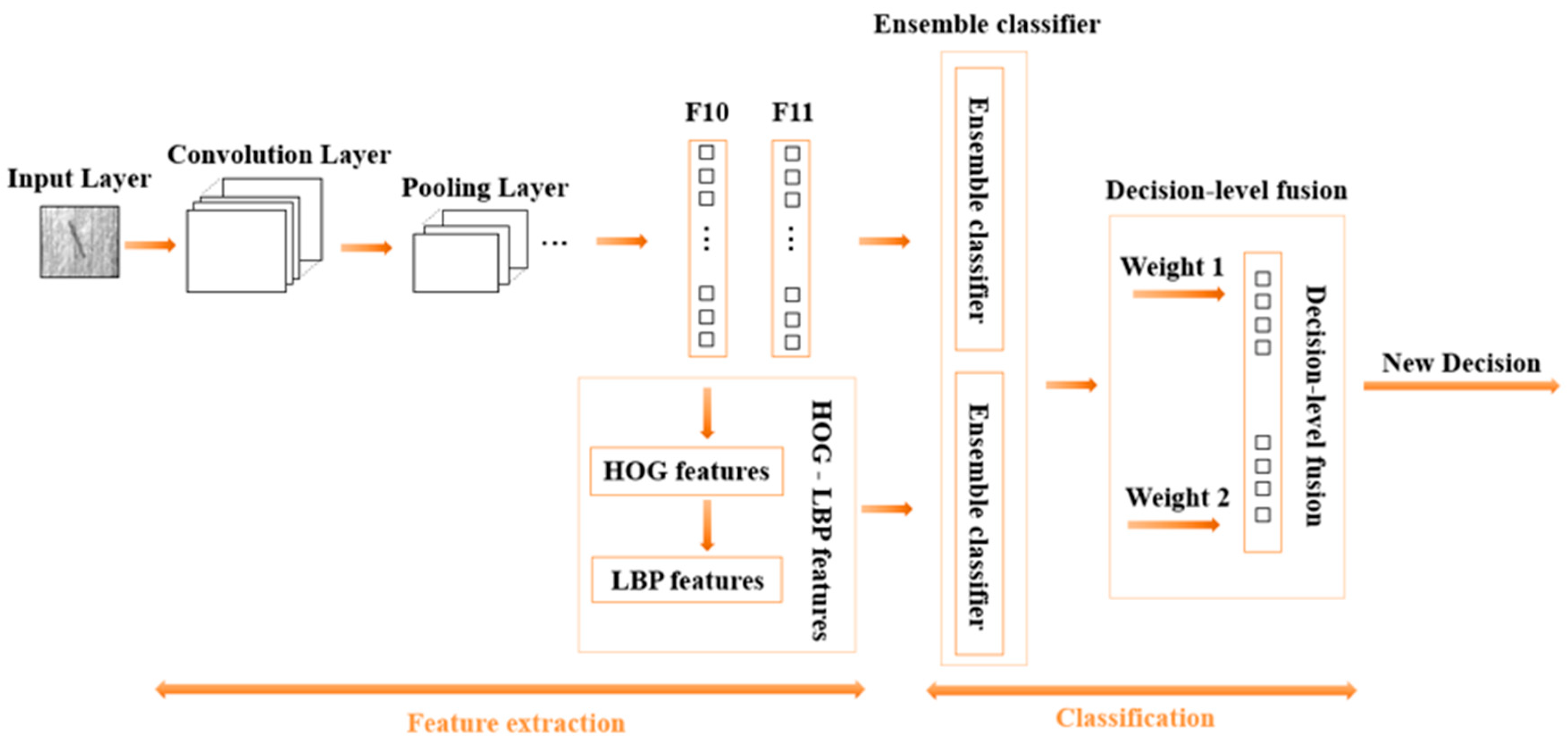
First, the size of the input image is 227 × 227. After the image is input into the neural network, it enters the first convolution layer. The convolution kernel is 11 × 11 pixels and the step size is 4. Then, the pooling operation is performed. The pooling window size of the first pooling layer is 3 and the step size is 2. The pooling operation is to reduce the dimension of the feature, and then a layer of convolution operation and a layer of pooling operation are performed; the convolution kernel of the convolution layer is 5 × 5 pixels, the step size is 1; the pooling window of the pooling layer is 3, the step size is 2; and then the operation of the three-layer convolution layer is performed, and their convolution kernels and step size is the same; the convolution kernel is 3 × 3 pixels and the step size is 1, then the last layer of the pooling layer operation is performed. The pooling window size is 3 and the step size is 2. The fully connected layer is performed after the pooling operation; the first fully connected layer summarizes all the features extracted by the above convolution layers and pooling layers. When the features enter the second fully connected layer, two branch operations are performed. The first branch is to use the HOG to extract the second fully connected layer, and then uses the LBP to further extract the HOG features; the output feature is called the HOG–LBP feature, which has strong robustness. In the symmetric ensemble classifier, the first ensemble classifier is used to classify the HOG–LBP feature. The second branch uses the second ensemble classifier to classify the third fully connected layer. The classification results of the symmetry branches ensemble classifier are fitted to the posterior probability of the target category; the classification results of each classifiers are used to calculate the decision weights. Finally, the decision weights are used for the symmetry ensemble classifier decision-level fusion. The output of the decision-level fusion is used as a new classification decision. The framework of the MDF-CNN is shown in Figure 1.

3. Experimental Results and Discussions

3.1. Datasets

The construction of the workpiece surface defect data set can be divided into two parts: image acquisition and data enhancement.

(1) Image acquisition:

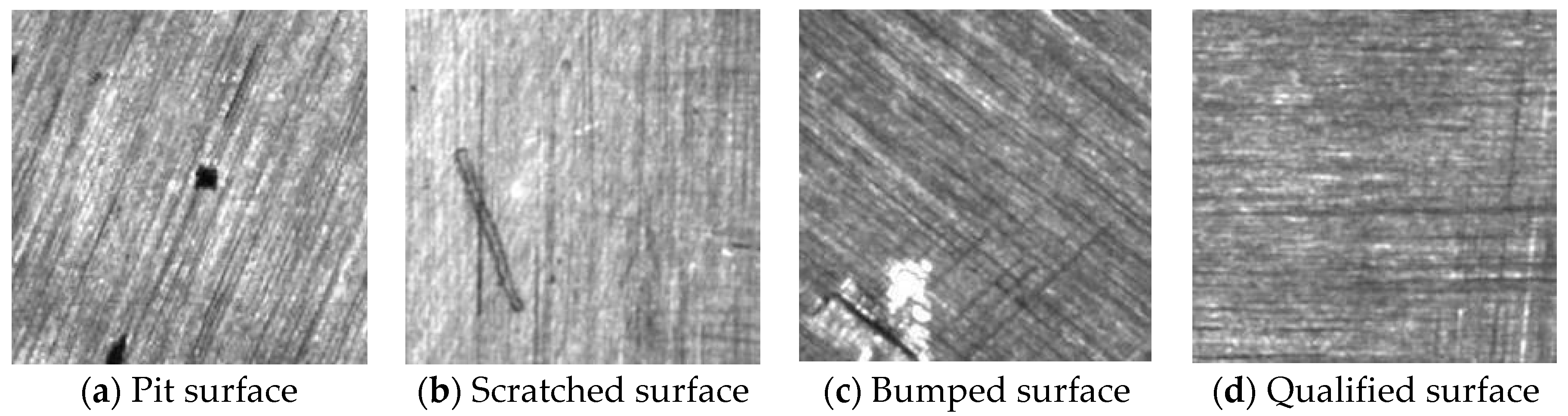
The experiments in this paper mainly focus on flat metal workpieces; the types of typical surface defects are pits, scratches and bumps, and the workpiece is milled. Defective workpieces are classified by quality inspection workers, which obtains 400 workpiece surface samples through the inspection system. The defective surfaces and the qualified surfaces are shown in Figure 2.

(2) Data enhancement:

To prevent over-fitting during the training process, the data samples are amplified, and the sample collection is performed by adjusting the hardware conditions of the collection environment, such as adjusting the intensity of the LED light source to change the lighting conditions, and rotating the workpiece to change the current position of the defect area. The number of the expanded image samples is 4600, which are the initial collection of the original workpiece surface. Manually selecting 2000 samples are used as the test set; the remaining 2600 samples are used as the training set.

The proportion of each defect type is shown in

Table 3. The test set.

Type	Parameter Value
Pit	500
Scratched surface	500
Bumped surface	500
Qualified surface	500
Total	2000

.

3.2. Hardware Platform

The used computer configuration was an Intel Xeon E5-1620 v3 3.5 GHz CPU, Quadro K2200 GPU, 8 G memory and 1 T hard disk capacity, and the GPU was used to accelerate the computation. The specific parameters of the industrial camera are shown in

Table 4. Industrial camera parameters.

Parameter	Parameter Value
Resolution	1280 × 960
Interface	Gigabit Ethernet
Pixel size	3.75 μm × 3.75 μm
Transmission distance	100 m
Maximum frame rate	40 fps

.

3.3. Performance Comparison

To prove the proposed model superiority, the proposed model is compared with some existing CNNs and the most advanced classification models for workpiece surface defects. The four defect types of normal, pit, scratch and bumped surfaces are used. The performance comparisons are shown in

Table 5. Performance comparisons.

Model	Accuracy
KNN	32.85%
MLP	25%
CNN	96.55%
CNN-SVM	96.90%
MDF-CNN	97.60%

; it can be seen that the proposed MDF-CNN has a higher classification accuracy than other models. The amount of parameters of the MLP and KNN algorithms is too large, which results in a huge calculation. Therefore, the detection accuracy is low: the accuracy of MLP is 25% and the accuracy of KNN is 32.85%. The CNN has a good detection effect in the field of defect detection. The accuracy of the CNN detection is 96.55%, while the detection accuracy of the proposed MDF-CNN model is 97.6%. The accuracy of the CNN-SVM model is 96.90%, the accuracy of the MDF-CNN model increased from 96.90% to 97.60% compared with the CNN-SVM model. Therefore, the proposed classification model has a higher generalization ability.

To further verify the effectiveness of the proposed algorithm, the MDF-CNN and other CNN models are used for comparison and verification in this experiment, as shown in

Table 6. Comparative experiments with other CNN models.

Model	Accuracy	Time (s)
AlexNet	96.55%	21.44
VGG16	96.40%	91.3
MDF-CNN	97.60%	24.47

. It can be seen that AlexNet is also used in the case of transfer learning. The classification accuracy is 96.55%, the detection time is 21.44 s, the VGG16 classification accuracy is 96.4% and the detection time is 91.3 s, which indicates that the VGG16 classification accuracy is not only lower than Alexnet, but also the complexity of the algorithm and the consumed time are the highest, which shows that merely deepening the network level cannot effectively improve the classification accuracy. The proposed MDF-CNN model has the highest classification accuracy, with a classification accuracy of 97.6%.

To further verify the effectiveness of the proposed algorithm, the comparison and verification experiment is carried out by using the MDF-CNN and other defect detection method, which is shown in

Table 7. Compared with other defect detection methods.

Model	Accuracy
SVM	50.20%
Decision tree	41.05%
MDF-CNN	97.60%

. It can be seen from the table that the classification accuracy of the SVM algorithm proposed in Reference [7] is 50.20%, and the classification accuracy of the decision tree algorithm proposed in Reference [9] is 41.05%; the MDF-CNN has the highest classification accuracy, with a classification accuracy of 97.6%.

3.4. Comparative Experiments of the Proposed Model with Different Kernel Functions

Although SVM is used as the basis weak classifier in the proposed model and the feature extraction degree is high, there are still nonlinear conditions. The feature extraction need be converted into a high-dimensional space to deal with nonlinear conditions. Kernel functions are adopted to avoid these problems.

In this section, the experiments are performed to compare and analyze the performances of the SVM, the CNN–SVM, the CNN and MDF-CNN with different kernel functions, such as linear kernel, polynomial kernel and RBF kernel, which are shown in

Table 8. The comparative experiments of different kernel functions.

Kernel	SVM	CNN-SVM	MDF-CNN
linear	48.15%	96.55%	97.55%
polynomial	50.20%	96.85%	97.60%
RBF	25%	25.25%	26.35%

. It can be seen that when using the polynomial kernel function, the detection accuracy of the SVM, the CNN-SVM and the proposed MDF-CNN model is the highest.

3.5. Effectiveness of Symmetry Ensemble Classifier

To demonstrate the effectiveness of the symmetry ensemble classifier, experiments are conducted to compare the performances of the MDF-CNN without and with a symmetry ensemble classifier combined with the SVM, which are shown in

Table 9. The MDF-CNN model without and with the symmetry ensemble classifier.

Model	Accuracy
MDF-CNN without symmetry ensemble classifier	97.00%
MDF-CNN with symmetry ensemble classifier	97.60%

. It can be seen that the symmetry ensemble classifier is useful for the MDF-CNN, in that the symmetry ensemble classifier can automatically combine weak classifiers with a high classification accuracy and is not prone to overfitting.

4. Conclusions

A workpiece surface defects classification model using a multi-classifier decision-level fusion classification based on a convolutional neural network is proposed in this paper. The HOG-LBP feature extraction is used to assist the CNN. The output results of the symmetry ensemble classifier are fitted to the posterior probability of the target category. The decision weight of each classifier is generated from the correct classification rate, which can be obtained and normalized by each classifier. Decision weights are used to perform decision-level fusion, and the traditional feature extraction method is effectively combined. Extensive experiments on multiple workpiece surface defects datasets show that the proposed model can effectively classify the workpiece surface defects, yield a good generalization ability and outperform the state-of-the-art methods.

References

- Jeffrey, K.; Feng, C. Automated defect inspection system for CMOS image sensor with micro multi-layer non-spherical lens module. J. Manuf. Syst. 2017, 45, 248–259. [Google Scholar] [CrossRef]
- Zhang, X.W.; Ding, Y.Q.; Lv, Y.Y. A vision inspection system for the surface defects of strongly reflected metal based on multi-class SVM. Expert Syst. Appl. 2011, 38, 5930–5939. [Google Scholar]
- Wang, P.; Zhang, X.; Mu, Y. The Copper Surface Defects Inspection System Based on Computer Vision. In Proceedings of the Fourth International Conference on Natural Computation, Jinan, China, 18–20 October 2008; pp. 535–539. [Google Scholar]
- Zhou, S.; Chen, Y.P.; Zhang, D.L. Classification of surface defects on steel sheet using convolutional neural networks. Mater. Tehnol. 2017, 51, 123–131. [Google Scholar] [CrossRef]
- Chu, M.X.; Jie, Z.; Liu, X.P. Multi-class classification for steel surface defects based on machine learning with quantile hyper-spheres. Chemom. Intell. Lab. Syst. 2017, 168, 15–27. [Google Scholar] [CrossRef]
- Bandhu, A.; Roy, S.S. Classifying multi-category images using deep learning: A convolutional neural network model. In Proceedings of the IEEE International Conference on Recent Trends in Electronics, Bangalore, India, 19–20 May 2017; pp. 915–919. [Google Scholar]
- Wang, Y.; Guo, H. Weld Defect Detection of X-ray Images Based on Support Vector Machine. IETE Tech. Rev. 2014, 31, 137–142. [Google Scholar] [CrossRef]
- Cui, D.Y.; Xia, K.W. Strip surface defects recognition based on PSO-RS&SOCP-SVM algorithm. Math. Probl. Eng. 2017, 2017, 1–9. [Google Scholar]
- Mohamed, A.; Hamdi, M.S.; Tahar, S. Decision Tree-Based Approach for Defect Detection and Classification in Oil and Gas Pipelines. In Proceedings of the Future Technologies Conference, Vancouver, BC, Canada, 13–14 November 2018; pp. 490–504. [Google Scholar]
- Zheng, T.; Jie, G.; Zhang, H.T. Innovative method for recognizing subgrade defects based on a convolutional neural network. Constr. Build. Mater. 2018, 169, 69–82. [Google Scholar]
- Wang, G.; Liao, T.W. Automatic identification of different types of welding defects in radiographic images. NDT E Int. 2002, 35, 519–528. [Google Scholar] [CrossRef]
- Suvdaa, B.; Ahn, J.; Ko, J. Steel surface defects detection and classification using SIFT and voting strategy. Int. J. Softw. Eng. Appl. 2012, 6, 161–166. [Google Scholar]
- D’Angelo, G.; Rampone, S. Feature extraction and soft computing methods for aerospace structure defect classification. Measurement 2016, 85, 192–209. [Google Scholar] [CrossRef] [Green Version]
- Rawat, W.; Wang, Z. Deep convolutional neural networks for image classification: A comprehensive review. Neural Comput. 2017, 29, 2352–2449. [Google Scholar] [CrossRef] [PubMed]
- Paoletti, M.E.; Haut, J.M.; Plaza, J. A new deep convolutional neural network for fast hyperspectral image classification. ISPRS J. Photogramm. Remote Sens. 2018, 145, 120–147. [Google Scholar]
- Zhao, D.; Wang, T.Y.; Chu, F.L. Deep convolutional neural network based planet bearing fault classification. Comput. Ind. 2019, 107, 59–66. [Google Scholar] [CrossRef]
- Gu, J.X.; Wang, Z.H.; Kuen, J. Recent advances in convolutional neural networks. Pattern Recognit. 2018, 77, 354–377. [Google Scholar] [CrossRef] [Green Version]
- Vogado, L.H.S.; Veras, R.M.S.; Araujo, F.H.D. Leukemia diagnosis in blood slides using transfer learning in CNNs and SVM for classification. Eng. Appl. Artif. Intell. 2018, 72, 415–422. [Google Scholar] [CrossRef]
- Han, D.M.; Liu, Q.G.; Fan, W.G. A new image classification method using CNN transfer learning and web data augmentation. Expert Syst. Appl. 2018, 95, 43–56. [Google Scholar] [CrossRef]
- Zhong, S.S.; Fu, S.; Lin, L. A novel gas turbine fault diagnosis method based on transfer learning with CNN. Measurement 2019, 137, 435–453. [Google Scholar] [CrossRef]
- Fahad, L.; Yassine, R. Survey on semantic segmentation using deep learning techniques. Neurocomputing 2019, 338, 321–348. [Google Scholar]
- Tompson, J.; Goroshin, R.; Jain, A. Efficient object localization using Convolutional Networks. In Proceedings of the IEEE Conference on Computer Vision and Pattern Recognition, Boston, MA, USA, 8–10 June 2015; pp. 648–656. [Google Scholar]
- Raheja, J.L.; Kumar, S.; Chaudhary, A. Fabric defect detection based on GLCM and Gabor filter: A comparison. Optik 2013, 124, 6469–6474. [Google Scholar] [CrossRef]
- Krishnan, K.G.; Vanathi, P.T. An efficient texture classification algorithm using integrated Discrete Wavelet Transform and local binary pattern features. Cogn. Syst. Res. 2018, 52, 267–274. [Google Scholar] [CrossRef]
- Lahiani, H.; Neji, M. Hand gesture recognition method based on HOG-LBP features for mobile devices. Procedia Comput. Sci. 2018, 126, 254–263. [Google Scholar] [CrossRef]
- Munir, N.; Kim, H.J.; Park, J. Convolutional neural network for ultrasonic weldment flaw classification in noisy conditions. Ultrasonics 2019, 94, 74–81. [Google Scholar] [CrossRef] [PubMed]
- Zhang, Y.X.; You, D.Y.; Gao, X.D. Welding defects detection based on deep learning with multiple optical sensors during disk laser welding of thick plates. J. Manuf. Syst. 2019, 51, 87–94. [Google Scholar] [CrossRef]
- Liu, R.X.; Yao, M.H.; Wang, X.B. Defects Detection Based on Deep Learning and Transfer Learning. Metall. Min. Ind. 2015, 7, 312–321. [Google Scholar]
- Dalal, N.; Triggs, B. Histograms of Oriented Gradients for Human Detection. In Proceedings of the IEEE Computer Society Conference on Computer Vision and Pattern Recognition, San Diego, CA, USA, 20–25 June 2005; pp. 886–893. [Google Scholar]
- Mahbod, A.; Chowdhury, M.; Smedby, Ö. Automatic brain segmentation using artificial neural networks with shape context. Pattern Recognit. Lett. 2018, 101, 74–79. [Google Scholar] [CrossRef]
- Ojala, T.; Pietikäinen, M.; Harwood, D.A. Comparative study of texture measures with classification based on featured distributions. Pattern Recognit. 1996, 29, 51–59. [Google Scholar] [CrossRef]
Figure 1.
The framework of the MDF-CNN.
Figure 2.
Typical surface defects and a normal surface.