Kane’s Formalism Used to the Vibration Analysis of a Wind Water Pump

Abstract

The paper uses Kane’s formalism to study two degrees of freedom (DOF) mechanisms with elastic elements = employed in a wind water pump. This formalism represents an alternative, in our opinion, that is simpler and more economical to Lagrange’s equation, used mainly by researchers in this type of application. In the problems where the finite element method (FEM) is applied, Kane’s equations were not used at all. The automated computation causes it to be reconsidered in the case of mechanical systems with a high DOF. Analyzing the planar transmission mechanism, these equations were applied for the study of an elastic element. An analysis was then made of the results obtained for this type of water pump. The matrices coefficients of the obtained equations were symmetric or skew-symmetric.

1. Introduction

The analytical mechanics gave, from the beginning, several equivalent formalisms useful in the analysis of mechanical systems with a large number of degrees of freedom (DOF). The advantage of these approaches lies in the fact that they are suitable for generalizations. However, in practice, despite a relatively large number of analysis possibilities, the Lagrange’s equation was used. The success of this method is based on the fact that it operates with classical and well-known notions of mechanics. However, due to the significant progress of the last five decades in the field of numerical computing methods and the use of computers in all domains, a reconsideration of these methods is required. Some of these formalisms can bring advantages in terms of modeling, writing algorithms, and computational time. The advantages and the drawbacks are summarized at the end of this section. By using a convenient method, it is possible to reduce the computing operations. For example, Hamilton’s method leads us to a system of first-order differential equations; therefore, there is no need to transform the second-order system of differential equations into a first-order system of differential equations.

The last decade shows us that we have begun to reconsider all the formalisms of analytical mechanics. This is a consequence of the desire to facilitate the representation of mathematical models and the need to reduce the amount of equations and steps that are required. Worldwide, there are different studies that have applied and analyzed alternative ways of obtaining the equations of motion. In the following, we show a summary of some of the most significant research studies on the subject.

Even if alternative methods were used in the analysis of multi body systems (MBSs), such as Gibbs–Appell equations, Hamilton equations, Maggi’s equations, Jacobi’s equations, Kane’s equations, etc., for problems that required the application of the finite element method (FEM) method, Lagrange’s equations were used almost exclusively. The disadvantage is the high level of calculus due to the large number of DOF. It is natural, therefore, to identify the most advantageous methods in terms of volume and calculus time. We mention that, even though different methods were used, the resulting system of differential equations was the same.

Using the results presented in [1,2,3,4,5,6,7,8,9,10,11,12,13,14,15,16], the following conclusions can be formulated regarding the advantages and the drawbacks of modeling an elastic mechanical system using the equivalent formalism of analytical mechanics.

As a method currently used, the Lagrange’s equations (LE) method, preferred in the case of mechanical systems with a high DOF, has proven that it can be successfully applied to a wide range of situations. The main advantage of the method is that basic and well-known notions are used. In the finite element analysis (FEA) of MBS systems with elastic elements, this method has been used by almost all researchers. Mechanical systems modeled with various types of finite elements have been studied using this method. In the first step, the equations of motion are computed. The next step is the assembly of these equations, which implies the writing of the constraint conditions between the finite elements, expressed generally by non-holonomic conditions. This step is actually the elimination of Lagrange’s multipliers from the obtained algebraic differential system (DAE). It has been proven that the method of LE is convenient for many applications [1,2,3,4,5,6,7]. The use of other equivalent formulations in analytical mechanics has been only sporadically investigated in relation to these problems.

The most used method by researchers to study such systems is the Lagrange’s method. The main reason is the degree of generality and abstraction that this method allows (as opposed to the Euler method, where every liaison force must be introduced and determined), but also the fact that researchers are accustomed to it. A major disadvantage is the fact that one must determine the multipliers, which, for large systems, can become a difficult thing.

Gibbs–Appell (GA) equations, although rarely used in the study of mechanical systems, have obvious advantages in terms of the representation form to be used. Compared with LE, it has advantages regarding the required computation time [8].

The disadvantage is that researchers are less familiar with some notions, such as energy of accelerations. The GA formalism is useful for non-holonomic systems. Advantages of the GA method have been presented in studies related to the calculus of MBSs with rigid elements [9]. The final equations obtained by applying this method are identical to those obtained with LE, but the computational effort is lower [10]. The major advantage of the method is that Lagrange’s multipliers do not appear in the written equations; the method eliminates them directly and, as a result, the number of unknowns is lower [11]. These advantages have been observed by the researchers and, lately, the method tends to become a [12] procedure. Gibbs–Appell equations have the advantage that the level of calculus involved in the modeling process is smaller. On the other hand, this method involves the introduction of a notion that researchers are less accustomed to operate with, namely the energy of accelerations.

Most analytical methods lead to a system of second-order differential equations. To solve this kind of system using commercial software, it is necessary to transform it by introducing additional variables to a system of first-order differential equations. Hamiltonian mechanics allows obtaining a system of first order and thus shorter time is needed to solve it. In this way, a time-consuming stage in the process of transforming from second-order differential equation systems to first-order differential systems is avoided. However, the method has a disadvantage in the need to perform numerous preliminary calculations [16]. We do not know a concrete study of all the aspects involved in the use of this method.

The last years have revealed increasing interest from researchers for Maggi’s equations (ME), which were little applied and which are an alternative formalism to the other formalisms in analytical mechanics [13,14]. The interest is also generated by the development of modern mechanical manufacturing systems (robots and manipulators) [15]. In the case of the study of non-linear systems, the feedback linearization technique involves the application of ME. However, this method is rarely used, despite all these advantages, and is less familiar to researchers. The use of Maggi’s and Kane’s equations (two equivalent formulations of the same principles) has advantages in the analysis of non-holonomic systems. The liaison conditions, expressed linearly, can be used immediately in the equations of motion. It also has the advantage that the obtained equations no longer contain Lagrange multipliers or the liaison forces from the Newton–Euler equations.

The paper aims to analyze the possibility of using Kane’s equations to derive the equations of motion for a finite element and also to identify the advantages of this approach for the researchers.

In order to test the possibility of applying the method and to find the potential problems that might appear during its use, we made an application based on a planar mechanism.

2. Finite Element Kinematics

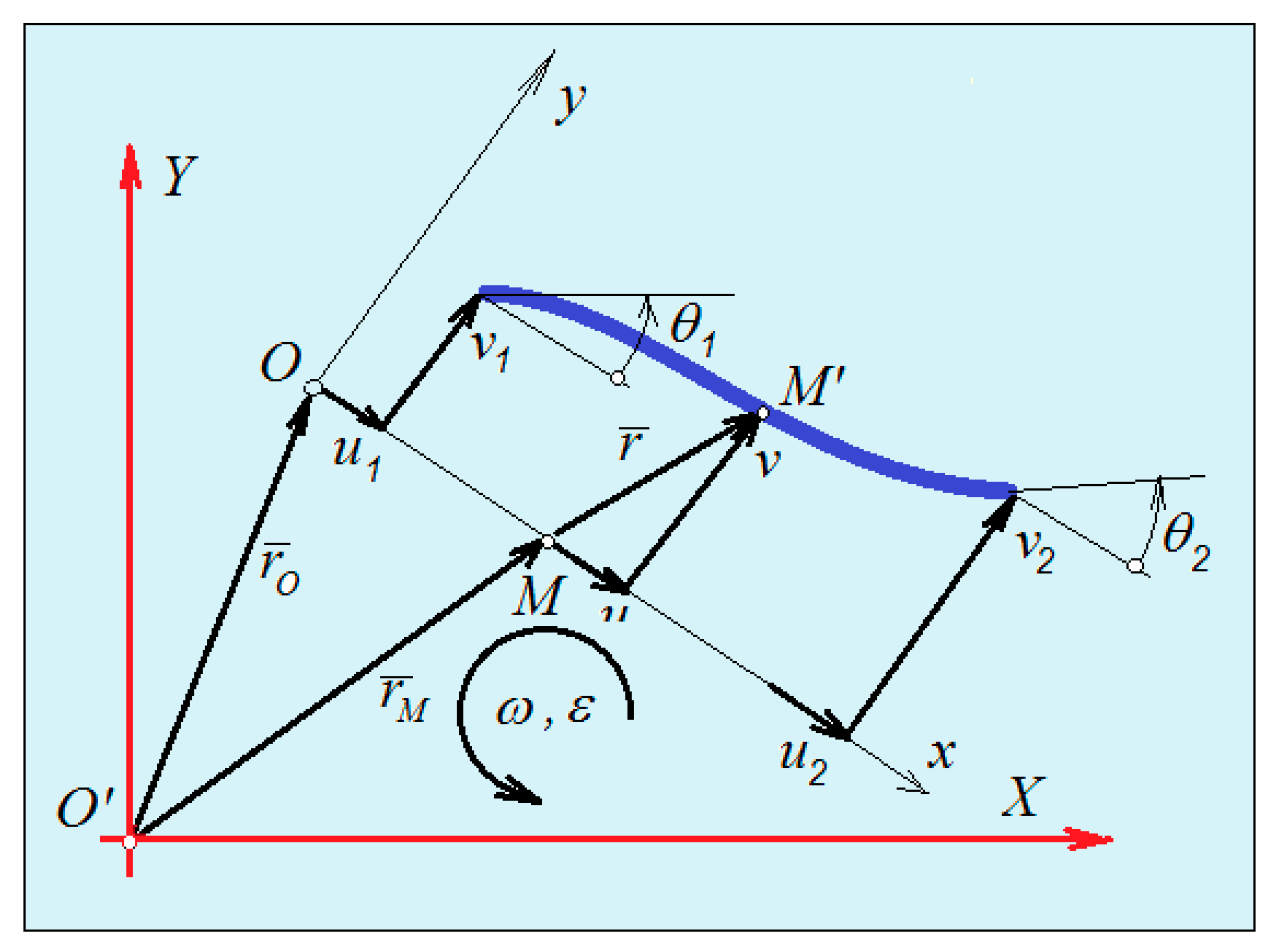
In our application, we used a one-dimensional finite element to study a planar mechanism with two degrees of freedom. To apply Kane’s equation (KE), it is necessary to know the kinematic of the element. In such analysis, the velocity and the acceleration of a point are of significant importance and are expressed in terms of nodal coordinates. An analysis of this problem can be found in [2,3,4,5,6]. The shape function that was used helped determine the displacements field in terms of independent nodal coordinates. (Figure 1)

The new position vector M’ of an arbitrary chosen point M becomes [7]:

$${\left\{r_{M^{\prime }}\right\}}_G={\left\{r_M\right\}}_G+{\left\{f\right\}}_G={\left\{r_M\right\}}_G+\left[R\right]\left\{\begin{array}{c}u\\ v\end{array}\right\}={\left\{r_o\right\}}_G+\left[R\right]\left\{\begin{array}{c}x\\ 0\end{array}\right\}+\left[R\right]\left[N\right]\left\{\delta \right\}$$

(1)

where $\left\{f(u,v)\right\}$ is the displacement vector; the shape functions are in $\left[N\right]=\left[\begin{array}{c}{N}_{\left(u\right)}\\ N_{\left(v\right)}\end{array}\right]=\left[\begin{array}{c}{N}_{\left(1\right)}\\ N_{\left(2\right)}\end{array}\right]$, and $\left\{\delta \right\}=\left\{\begin{array}{c}{\delta }_1\\ {\delta }_2\end{array}\right\}$ and $\left\{{\delta }_1\right\}$, $\left\{{\delta }_2\right\}$ are the displacement vectors. The slope is [6]:

$$\beta =\frac{dv}{dx}=\frac{d}{dx}\left(\left[N_{(v)}\right]\left\{{\delta }_e\right\}\right)=\left[N_{(v)}^{\prime }\right]\left\{{\delta }_e\right\}$$

(2)

With G index, we denote a vector or a matrix with components in the global coordinate system, and with L index, we denote a size with components in the local system.

From Equation (1), the velocity of a point results in:

$${\left\{v_{M^{\prime }}\right\}}_G={\left\{{\dot{r}}_{M^{\prime }}\right\}}_G={\left\{v_O\right\}}_G+\left[\dot{R}\right]{\left\{\begin{array}{c}x\\ 0\end{array}\right\}}_L+\left[\dot{R}\right]\left[N\right]{\left\{\delta \right\}}_L+\left[R\right]\left[N\right]{\left\{\dot{\delta }\right\}}_L$$

(3)

Calculated in [6,7], where ${\left\{v_O\right\}}_G={\left\{{\dot{r}}_O\right\}}_G$ is the velocity vector of the origin of the mobile coordinate system.

The transformation of a vector is performed by the matrix $\left[R\right]$:

$${\left\{t\right\}}_G=\left[R\right]{\left\{t\right\}}_L$$

(4)

In Appendix A are presented more results used in the paper.

3. Kane’s Equations Used in Conjunction with FEA

Kane’s method and equations have represented, during the last decades, a method that was successfully applied in the study of MBS systems. The KE method can be used for both holonomic and non-holonomic systems and can eliminate some of the disadvantages of classical methods in analytical mechanics (Newton–Euler and Lagrange). From a theoretical point of view, Maggi and Kane equations are equivalent, representing the same method very well suited for systems with non-holonomic constraints [17]. The application of Kane’s equations was determined by the need to study complex flexible structures such as robots and manipulators [18]. It has been found that applying this method allows efficient calculation for these systems [19,20,21,22]. The advantage of these equations is that they do not contain constraints forces [23]. The paper presents the necessary formalism to derive the motion equation for a finite element. A planar mechanism is studied, but the method can be applied for every type of an elastic MBS. Of course, the specific form of the equations must be calculated each time considering the shape functions required by the specific finite element chosen.

A short presentation of the Kane’s equations is presented in Appendix B. For an elastic finite element, considered as a solid, the Kane’s equation can be written as:

$${\displaystyle \sum _{i=1}^N{\overline{F}}_i\frac{\partial {\overline{v}}_i}{\partial {\dot{q}}_k}}={\displaystyle \underset{V}{\int }\overline{a}}\frac{\partial \overline{v}}{\partial {\dot{q}}_k}dmk=\overline{1,n}$$

(5)

where by $k=\overline{1,n}$ is meant $k=1,2,\dots \dots ,n$.

Differentiating the expression of velocity Equation (3), we obtain:

$${\left\{a_{M^{\prime }}\right\}}_G={\left\{a_o\right\}}_G+\left[\ddot{R}\right]\left\{\begin{array}{c}x\\ 0\end{array}\right\}+\left[\ddot{R}\right]\left[N\right]{\left\{\delta \right\}}_L+2\left[R\right]\left[N\right]{\left\{\dot{\delta }\right\}}_L+\left[R\right]\left[N\right]{\left\{\ddot{\delta }\right\}}_L$$

(6)

From Equation (1), we obtain:

$$\frac{\partial {\left\{{v^{\prime }}_M\right\}}_G}{\partial {\left\{\dot{\delta }\right\}}_L}=\left[R\right]\left[N\right]\mathrm{and}{\left(\frac{\partial {\left\{{v^{\prime }}_M\right\}}_G}{\partial {\left\{\dot{\delta }\right\}}_L}\right)}^T={\left[N\right]}^T{\left[R\right]}^T$$

(7)

The expression $\frac{\partial \left\{T\right\}}{\partial \left\{\delta \right\}}$, if $\left\{T\right\}=\left[A\right]\left\{\delta \right\}$, is $\left[A\right]$. It is possible to write:

$${\left(\frac{\partial {\left\{v_{M^{\prime }}\right\}}_G}{\partial {\left\{\dot{\delta }\right\}}_G}\right)}^T{\left\{a_{M^{\prime }}\right\}}_G={\left[N\right]}^T{\left[R\right]}^T{\left\{a_{M^{\prime }}\right\}}_G$$

(8)

$$\begin{array}{cc}& {\displaystyle \underset{V}{\int }{\left(\frac{\partial {\left\{v_{M^{\prime }}\right\}}_G}{\partial {\left\{\dot{\delta }\right\}}_G}\right)}^T{\left\{a_{M^{\prime }}\right\}}_G}=\left({\displaystyle \underset{V}{\int }\rho {\left[N\right]}^{T}dV}\right){\left\{a_O\right\}}_L+{\displaystyle \underset{V}{\int }{\left[N\right]}^T\left({\left[\epsilon \right]}_L+{\left[\omega \right]}_L{\left[\omega \right]}_L\right){\left\{r\right\}}_L\rho dV}+\hfill \\ \hfill +& \left({\displaystyle \underset{V}{\int }{\left[N\right]}^T\left({\left[\epsilon \right]}_L+{\left[\omega \right]}_L{\left[\omega \right]}_L\right)\left[N\right]\rho dV}\right){\left\{\delta \right\}}_L+2\left({\displaystyle \underset{V}{\int }\rho {\left[N\right]}^T{\left[\omega \right]}_L\left[N\right]dV}\right){\left\{\dot{\delta }\right\}}_L+\left({\displaystyle \underset{V}{\int }{\left[N\right]}^T\left[N\right]\rho dV}\right){\left\{\ddot{\delta }\right\}}_L\hfill \\ & =-\left[m_O^i\right]{\left\{a_O\right\}}_L-\left\{q^i(\epsilon )\right\}-\left\{q^i(\omega )\right\}+\left[k\left(\epsilon \right)\right]\left\{\delta \right\}+\left[k\left(\omega \right)\right]\left\{\delta \right\}+\left[c\left(\omega \right)\right]{\left\{\dot{\delta }\right\}}_L+\left[m\right]{\left\{\ddot{\delta }\right\}}_L\hfill \end{array}$$

(9)

The following notations were made:

$$\left[m\right]={\displaystyle \underset{V}{\int }{\left[N\right]}^T\left[N\right]\rho dV}=\left[m_{11}\right]+\left[m_{22}\right];\left[m_O^i\right]={\displaystyle {\int }_V\rho \left[N\right]d}V;$$

(10)

$$\left[c\left(\omega \right)\right]={\displaystyle \underset{0}{\overset{L}{\int }}{\left[N\right]}^T\left[{\omega }_L\right]\left[N\right]\rho Adx}=\omega \left(\left[m_{21}\right]-\left[m_{12}\right]\right);\left[k\left(\epsilon \right)\right]={\displaystyle \underset{0}{\overset{L}{\int }}{\left[N\right]}^T\left[{\epsilon }_L\right]\left[N\right]\rho Adx}=\epsilon \left(\left[m_{21}\right]-\left[m_{12}\right]\right);$$

(11)

$$\left[k\left(\omega \right)\right]=-{\displaystyle \underset{0}{\overset{L}{\int }}{\left[N\right]}^T{\left[\dot{R}\right]}^T\left[\dot{R}\right]\left[N\right]\rho Adx}={\displaystyle \underset{0}{\overset{L}{\int }}{\left[N\right]}^T\left[{\omega }_L\right]\left[{\omega }_L\right]\left[N\right]\rho Adx}=-{\omega }^2\left(\left[m_{11}\right]+\left[m_{22}\right]\right)$$

(12)

$$\left\{q^i\left(\epsilon \right)\right\}={\displaystyle \underset{0}{\overset{L}{\int }}{\left[N\right]}^T\left[{\epsilon }_L\right]\left\{\begin{array}{c}x\\ 0\end{array}\right\}\rho Adx}=\epsilon \left\{m_{2x}\right\};\left\{q^i\left(\omega \right)\right\}={\displaystyle \underset{0}{\overset{L}{\int }}{\left[N\right]}^T\left[{\omega }_L\right]\left[{\omega }_L\right]\left\{\begin{array}{c}x\\ 0\end{array}\right\}\rho Adx}={\omega }^2\left\{m_{1x}\right\}$$

(13)

We obtain:

$$\begin{array}{cc}\hfill \left[m\right]\left\{\ddot{\delta }\right\}+& 2\omega \left(\left[m_{21}\right]-\left[m_{12}\right]\right)\left\{\dot{\delta }\right\}+\left(\left[k_b\right]+\left[k_a\right]+\epsilon \left(\left[m_{21}\right]-\left[m_{12}\right]\right)-{\omega }^2\left(\left[m_{11}\right]+\left[m_{22}\right]\right)+\left[k^g\right]\right)\left\{\delta \right\}=\hfill \\ & =\left\{q^{ext}\right\}+\left\{q^{liaison}\right\}-\epsilon \left\{m_{2x}\right\}-{\omega }^2\left\{m_{1x}\right\}-\left[m_o^i\right]{\left\{{\ddot{r}}_o\right\}}_L\hfill \end{array}$$

(14)

In Equation (14), Equation (7) was applied. Thus, in a nodal point, k acts as generalized forces $\left\{F_k\right\}$ composed by the external forces (concentrated and distributed), the liaison forces, and the forces deriving from a potential. The corresponding velocities of these points can be found inside the velocities vector ${\left\{\dot{\delta }\right\}}_G$. We obtain:

$${\left(\frac{\partial {\left\{v_{M^{\prime }}\right\}}_G}{\partial {\left\{\dot{\delta }\right\}}_G}\right)}^T\left\{F_k\right\}\rho dV=\left(\left[k\right]+\left[k\left(\epsilon \right)\right]+\left[k\left(\omega \right)\right]+\left[k^g\right]\right){\left\{\delta \right\}}_L-{\left\{q^{ext}\right\}}_L-{\left\{q^{liaison}\right\}}_L$$

(15)

${\left\{q^{ext}\right\}}_L$ is the generalized external nodal forces vector, $\left(\left[k\right]+\left[k\left(\epsilon \right)\right]+\left[k\left(\omega \right)\right]+\left[k^g\right]\right){\left\{\delta \right\}}_L$—is the vector of forces deriving from a potential, ${\left\{q^{liaison}\right\}}_L$—is the liaison vector [6], and $\left\{v_{M^{\prime }}\right\}$ is, in this representation, the velocity of the nodal point k.

4. Study of a Planar Mechanism Used in a Wind Water Pump

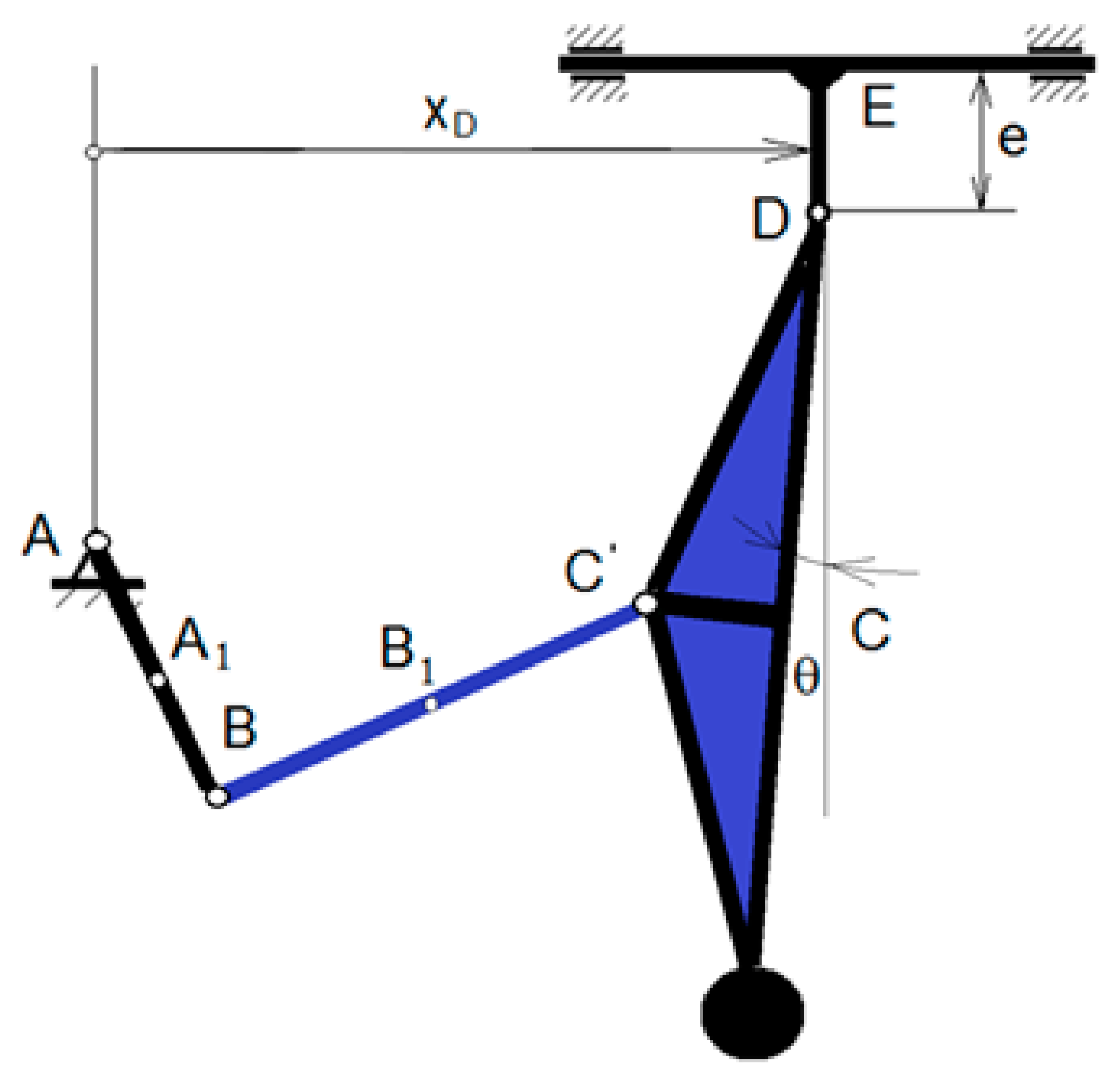
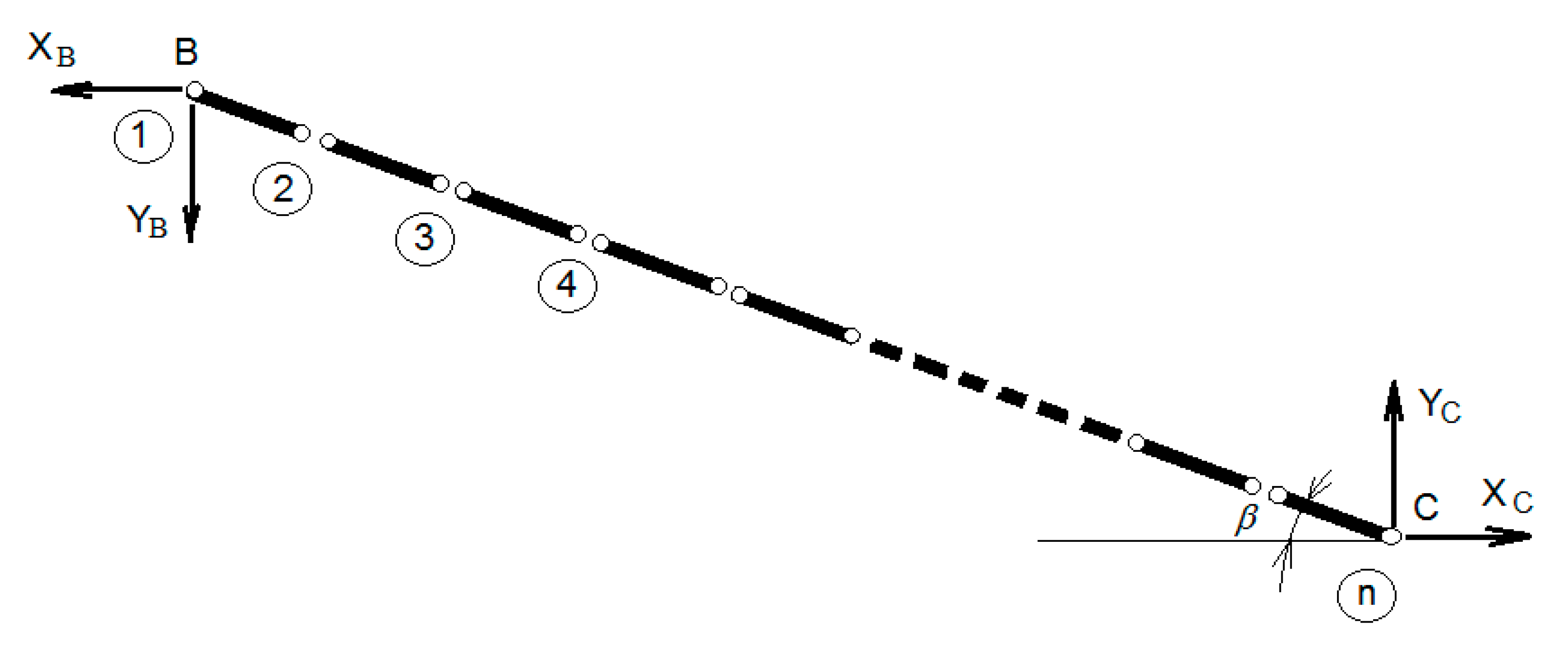
The mechanism of the transmission of the wind water pump is presented in Figure 2 [24]. The elements of the mechanism are rigid despite the B C’ beam, which is considered linear elastic.

To determine the constraint forces in the connection point, we consider all the elements of the mechanism being rigid (it is a first approximation, and we consider that the deformability of the beam does not influence the rigid body motion of the mechanism) [25,26]. In this case, if we know the moment offered by the electric engine and the friction in the joint after the integration of the equations, we can compute the liaison forces in the hinges B and C’. These forces can be introduced now in the finite element model.

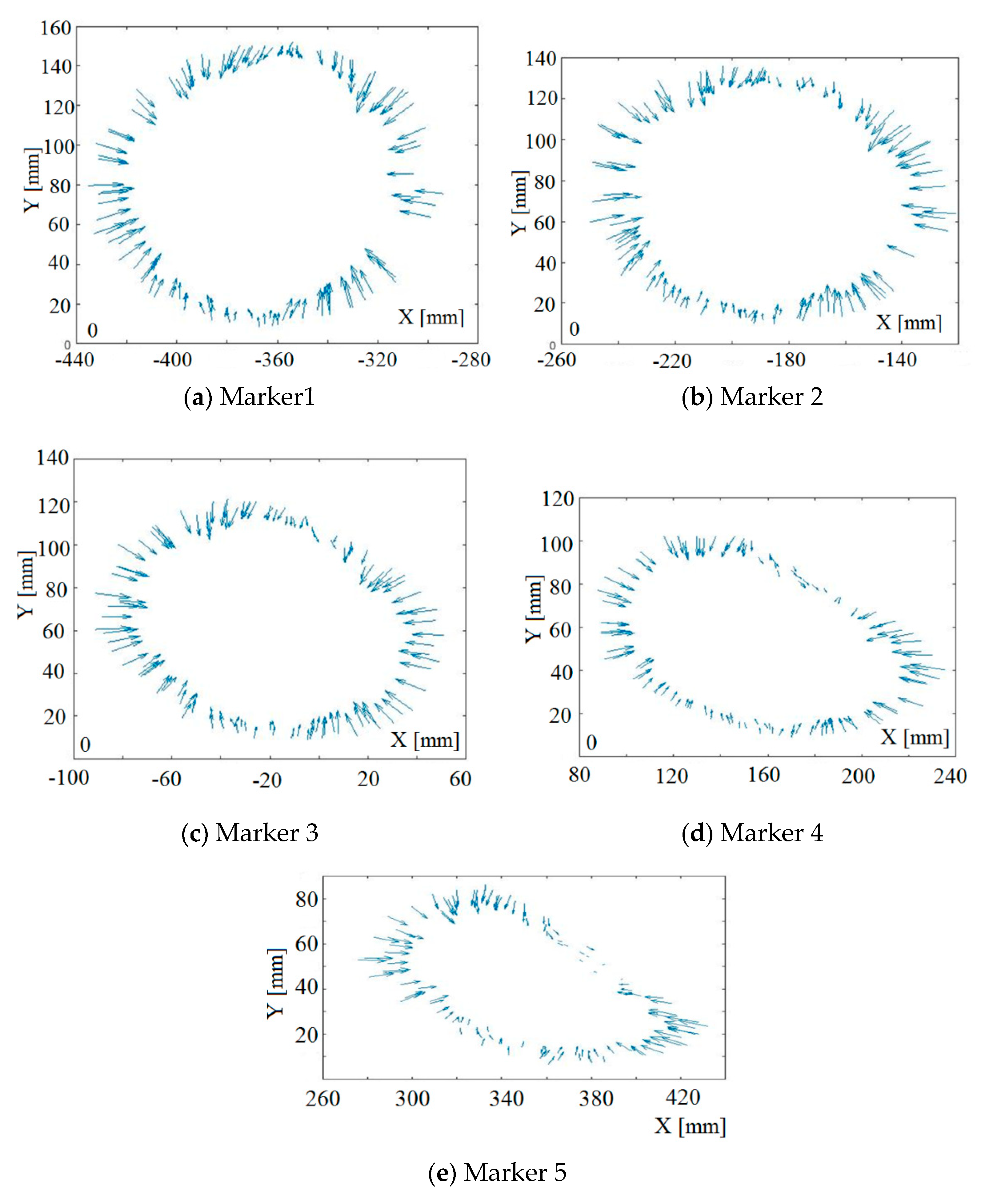
However, due to the many parameters that we have to take into account and which are difficult to determine or approximate, we used another method of determining the liaison forces. Recordings were made of the movement of some characteristic points of the mechanism, their trajectories were obtained, and, based on them, the speed and the acceleration fields of the mechanism were determined. Knowing the accelerations and the equations of motion, we could determine the forces that appeared in the two hinges (by solving a linear system) and use them in the finite element model.

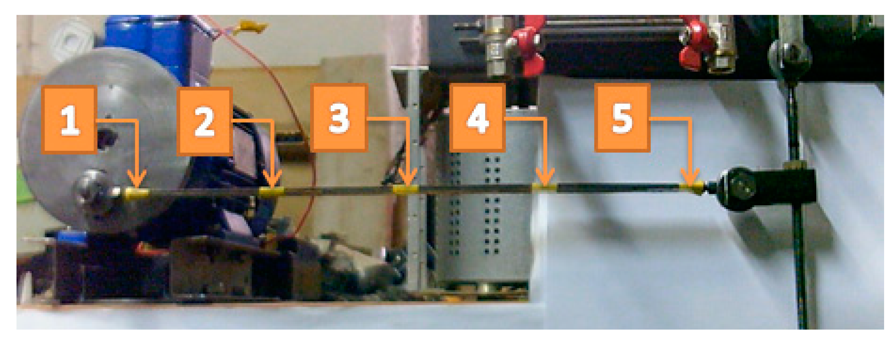
In Figure 3 are presented the points where the markers were glued. These forces are necessary for writing the equations of motion of the BC’ elastic beam. They were determined previously using Kane’s equations. After this step, we computed the free vibrations of the equation system that was obtained.

The markers placed on the bar were tracked using a video analysis and modeling program. Following the recording of the markers’ positions with the help of the analysis program, the speeds and the accelerations of the points were determined as well as the trajectories traveled by them.

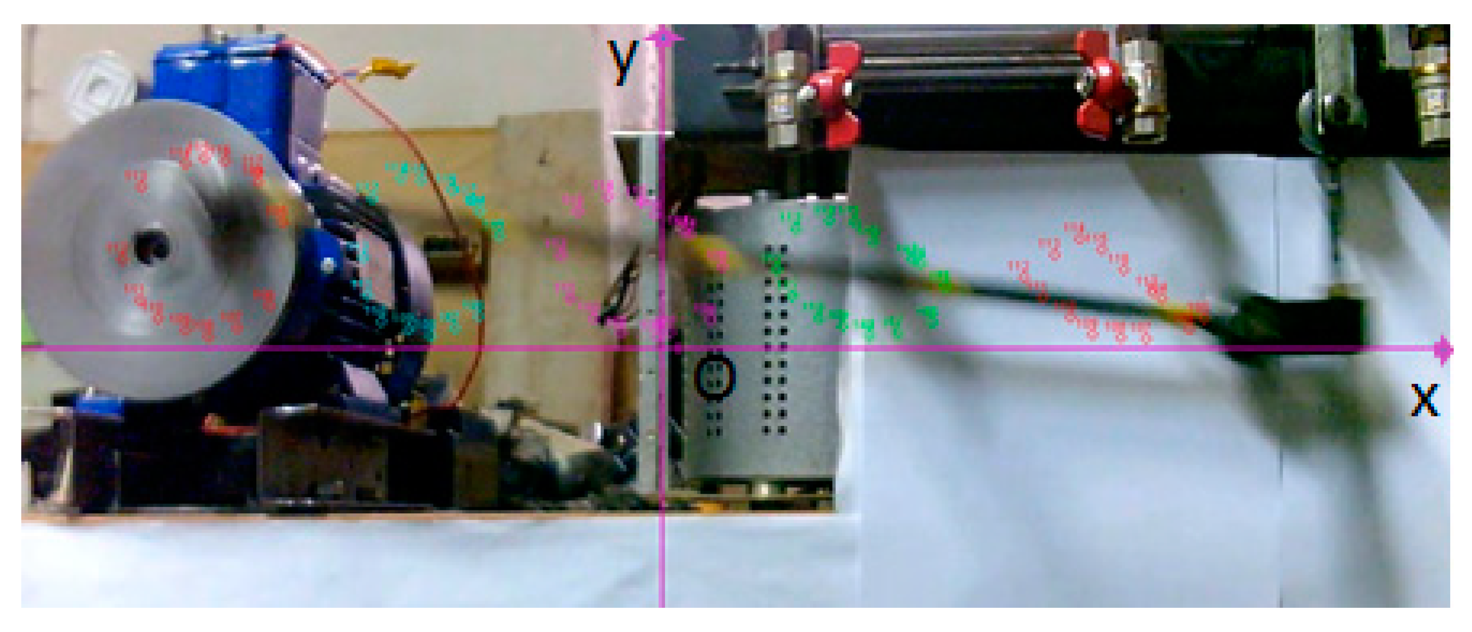
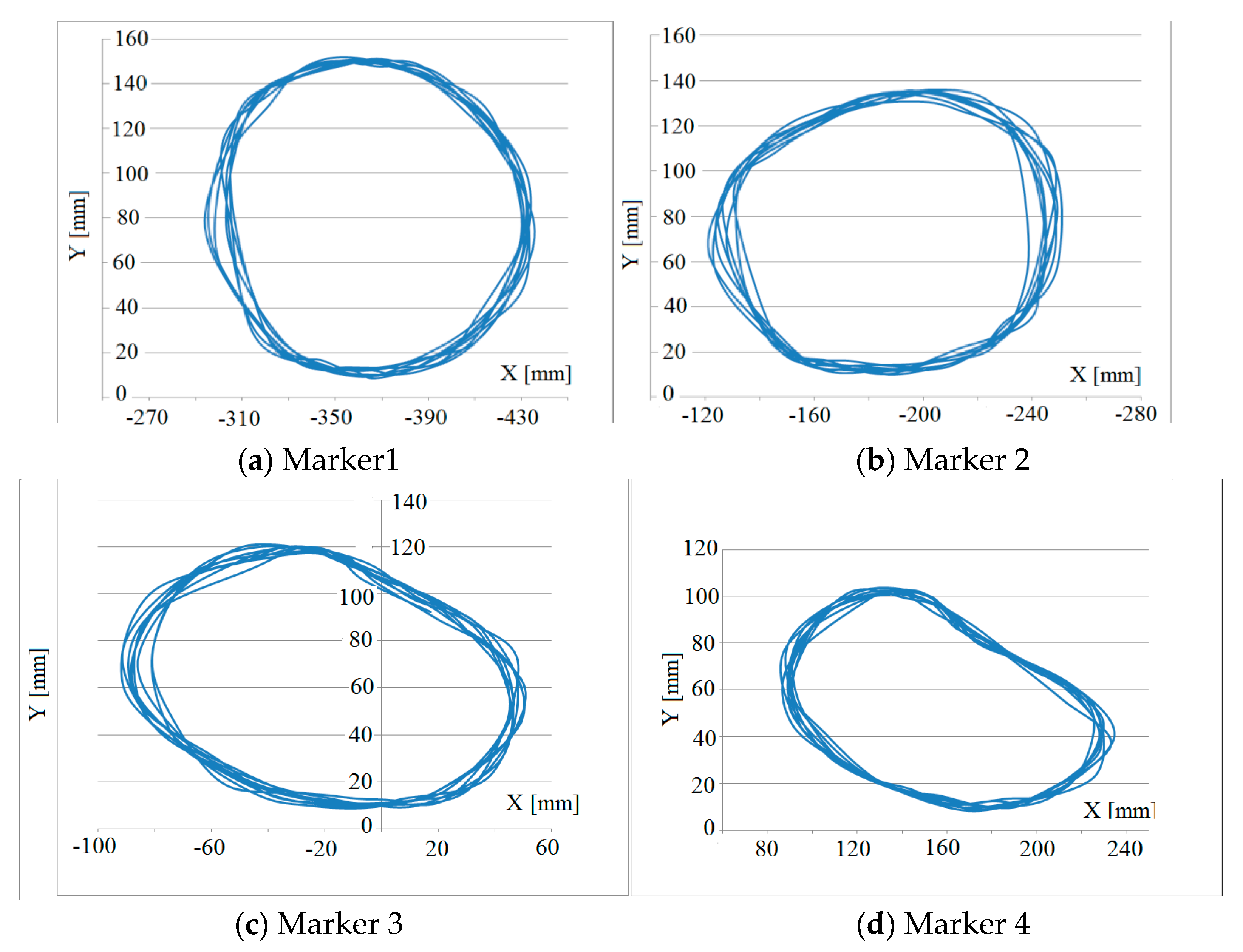
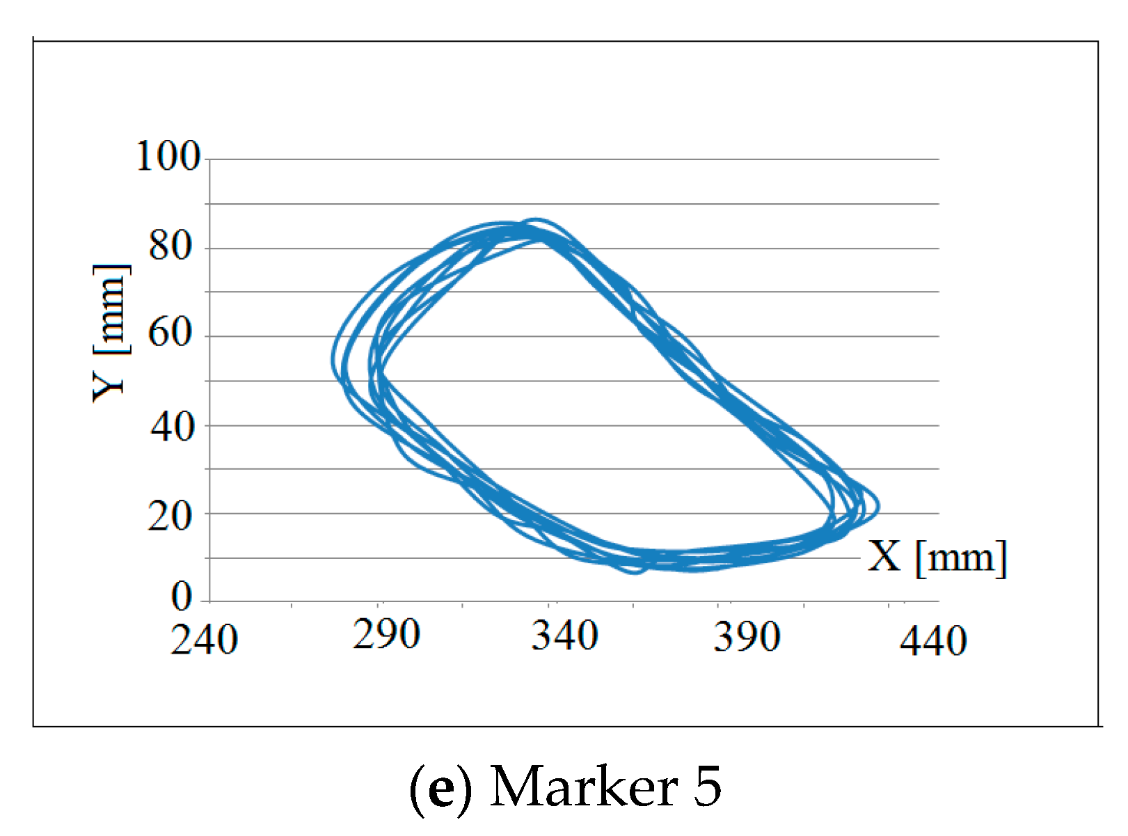
In Figure 4 are presented the trajectories of each chosen point on the bar using the data taken by the video analysis program. These are represented according to the positions given by the main coordinate axes of the chosen system, XOY, OX being the horizontal axis and OY the vertical axis.

For analysis and processing of the results as well as for the modeling with finite elements, simple codes written in MATLAB were used. This was done due to the simplicity and the versatility of this programming environment. Some of its advantages would be that it allows the easy implementation of algorithms, it is possible to develop codes easily, corrections can be made quickly, it allows the use of relatively large data sizes of the studied system, and it shows fast graphical results. The trajectories were presented in Figure 5.

The velocity and the acceleration fields (Figure 6) were determined using the aforementioned optical method. The acceleration fields are presented in the figures below for the five nodes studied.

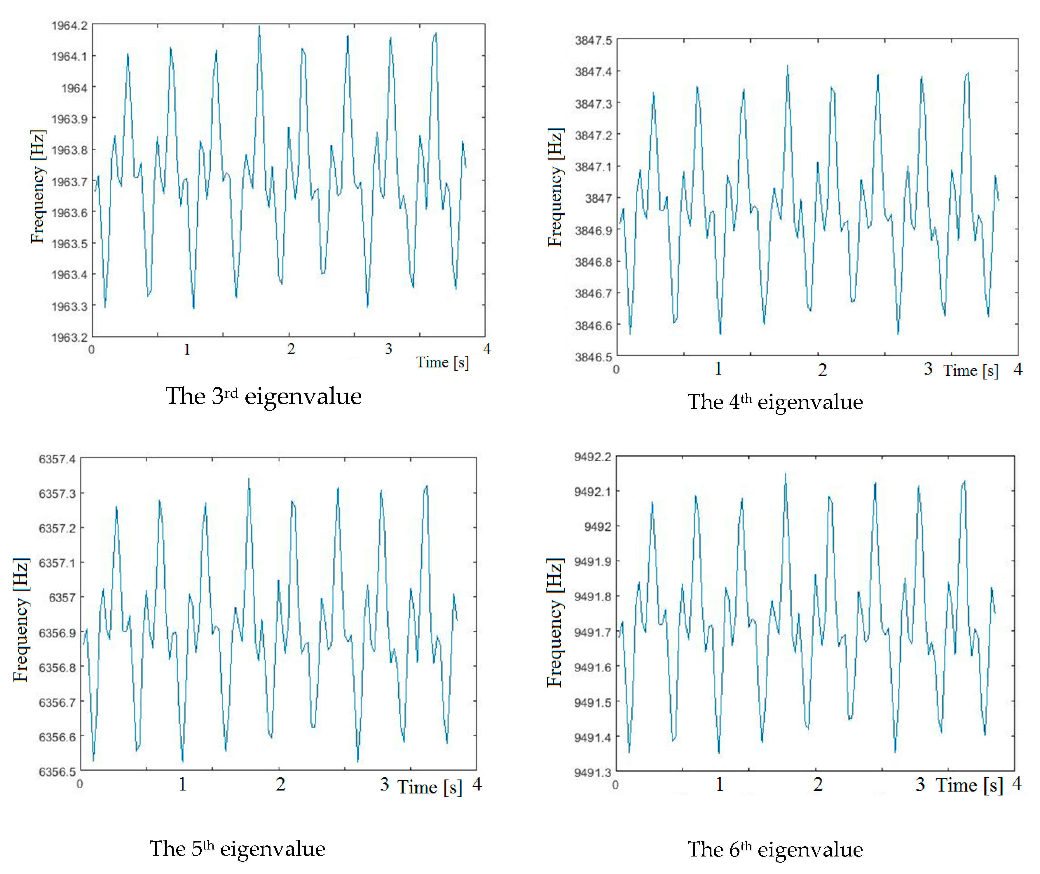
The model of the beam divided in finite elements is presented in Figure 7. In the hinge B and C, we could introduce the reactions previously determined using the optical measurement and solving the linear system of equation containing the reaction (liaison forces). Then, it was possible to perform a modal analysis of the beam. The results presented in the graphs below were taken for the same operating angular velocity, 140 rpm, this being the maximum speed at which experimental measurements were made (Figure 8).

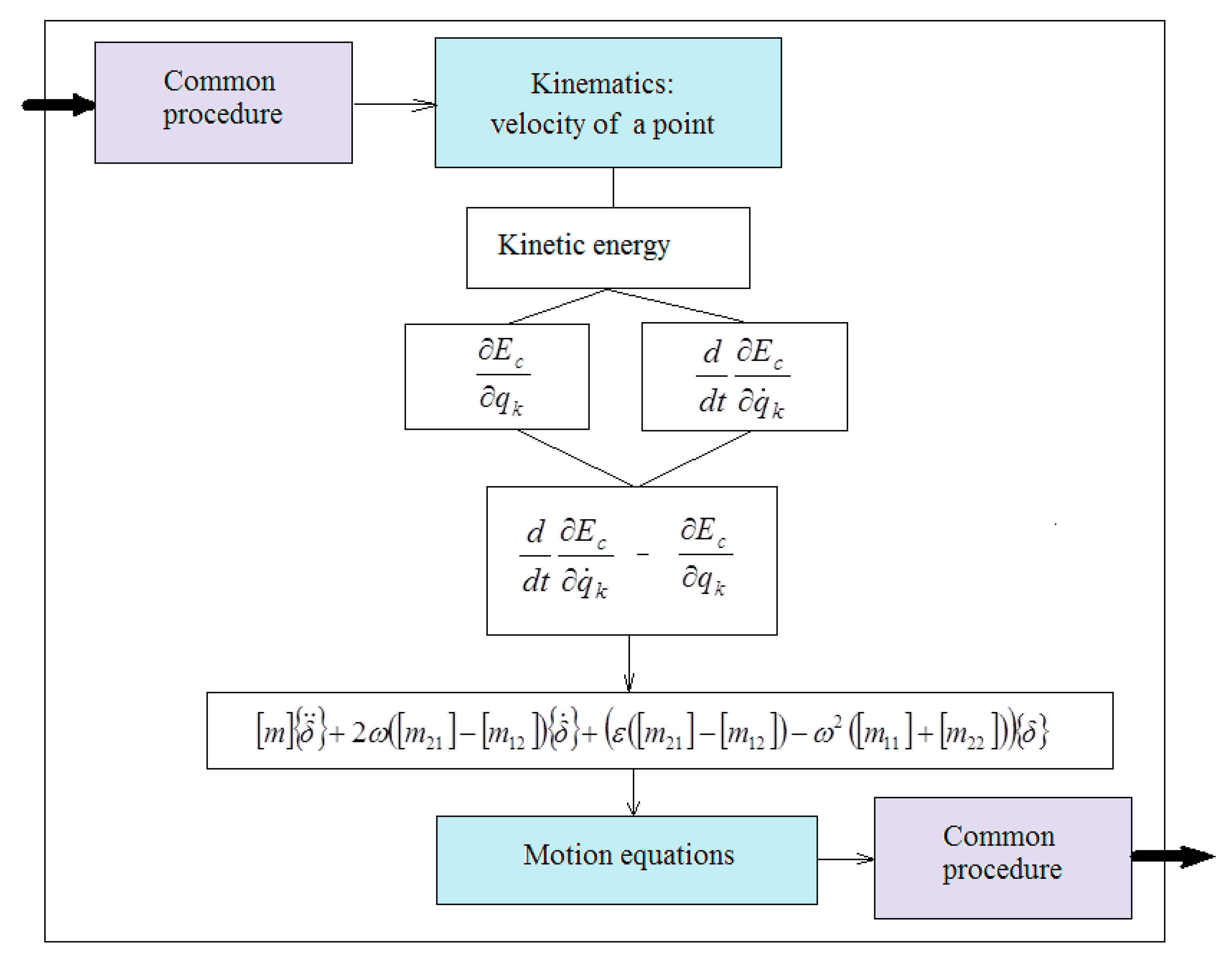
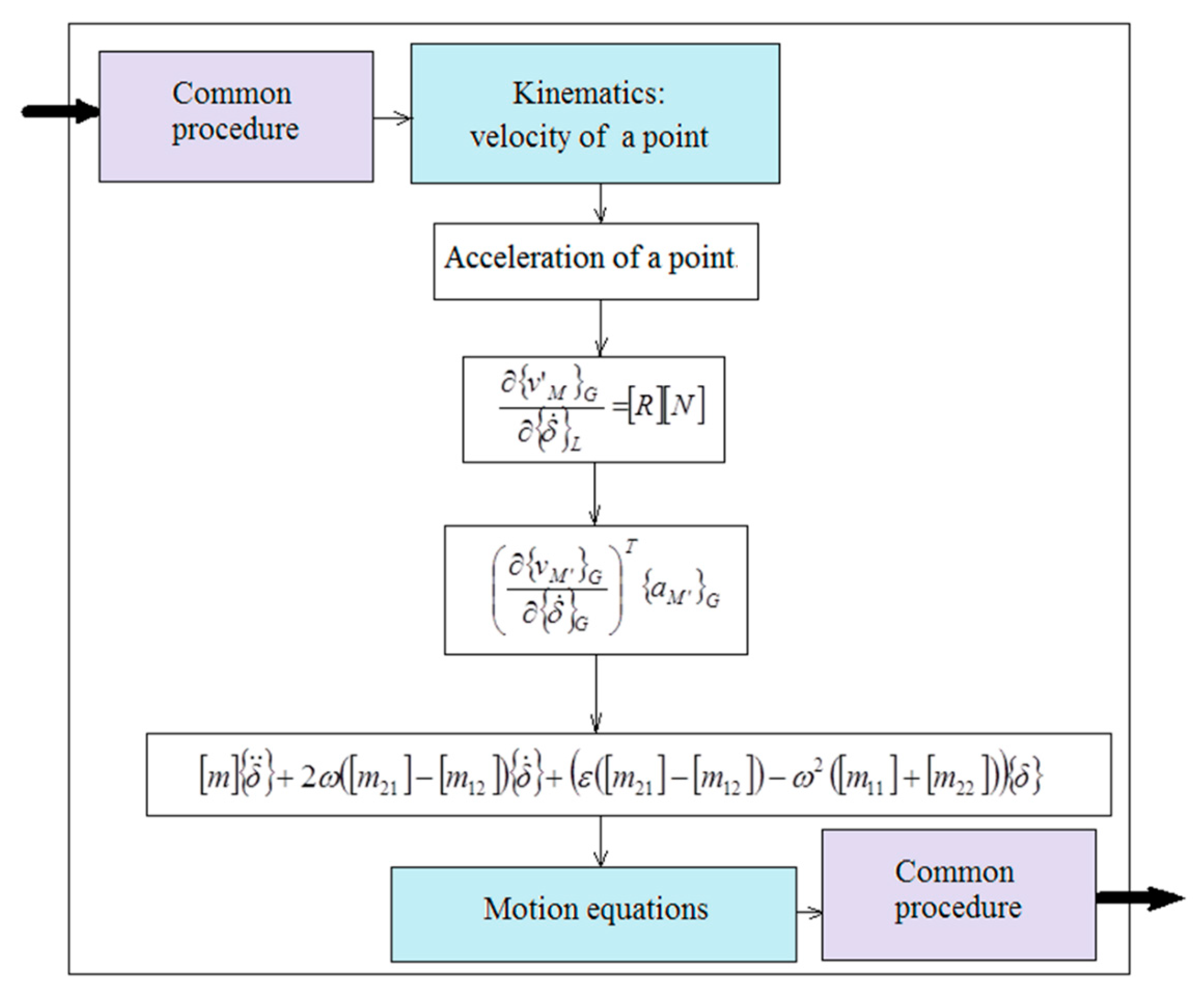
In the following, we try a comparison between the use of Kane’s and Lagrange’s equations based on reference books [27,28]. The procedure follows a series of similar steps. The differences occur when Lagrange’s formulas and Kane’s formulas are actually applied (Figure 9 and Figure 10). The number of distinctive operations in the two cases is studied. There are still elementary matrix operations, but we do not make the comparison there, considering that the number of terms in the case of Lagrange’s method is significantly higher than in the case of applying Kane’s method (

Table 1. Comparison between the numbers of operations for the two methods.

$\frac{\partial E_c}{\partial {\dot{q}}_k},\frac{\partial E_c}{\partial q_k}$			$\left(\frac{\partial {\left\{v_{M^{\prime }}\right\}}_G}{\partial {\left\{\dot{\delta }\right\}}_G}\right)$
Number of elements			Number of elements
1	10	30	1	10	30
Number of operations
78	1008	9486	6	33	93

).

From the analysis of the presented calculus, it was found that there was an obvious difference between the numbers of differences implied by the two methods. Apparently, the difference was very large and should have led to significant time savings if the method of Kane’s equations was applied. In reality, this step represented only a fraction of the multitude of operations necessary to perform. Consequently, the economy achieved was much smaller. For example, in the case of writing a calculus program in MATLAB for the calculation of the beam studied in the paper, which was discretized in 30 finite elements, the comparison led to a decrease in calculation time of only 7%.

5. Conclusions and Discussions

The literature studied suggests that LE presents some advantages for the researchers. The main disadvantage is the need to determine the Lagrange multipliers from the DAE obtained, which is difficult to achieve in the case of large DOF systems. This involves numerous calculations and large computational times. By comparison, the GA method seems to eliminate this disadvantage but introduces a new notion, energy of the accelerations. An alternative is ME, very useful when the constraints are non-holonomic. The last years have indicated an interest in researchers towards this method in the context of the need to study complex systems such as robots and manipulators applied at the present time on a large scale in the manufacturing industry. Hamiltonian formalism has the advantage of obtaining a system of first-order differential equations, which can become a plus in the case of using numerical calculation. However, the complexity of the intermediate calculations makes the method inconvenient for the researchers. The KE method, which is equivalent to the ME method, has begun to be used more widely in the last decade, with studies also led by the automation industry and industrial robots. In the paper, the KE formalism was applied to determine the dynamic response of an elastic MBS. The application considered was that of the transmission of a water pump driven by the wind. The finite element chosen was a one-dimensional element where classical third and fifth degree interpolation polynomials were used. It can be seen that KE can be a successful alternative in determining the equations of motion with the advantage of being economical. The uses of these equations present a natural alternative for non-holonomic mechanical systems. A comparison between the two methods was made in the paper. For the example highlighted in the paper, which is of small size, this difference may seem minor, but for large systems with high DOF, the difference may become significant.

Kane’s equations can be an economical and a simple alternative to the problem. The mentioned methods and the other known ones from the analytical mechanics with their equivalents will be re-evaluated in the context of the development of the modern industry, characterized by working mechanisms with high speeds and high loads. This implies the fact that new technologies and software development on these new methods are needed.

References

- Erdman, A.G.; Sandor, G.N.; Oakberg, A. A General Method for Kineto-Elastodynamic Analysis and Synthesis of Mechanisms. J. Eng. Ind. 1972, 94, 1193. [Google Scholar] [CrossRef]
- Nath, P.K.; Ghosh, A. Kineto-Elastodynamic Analysis of Mechanisms by Finite Element Method. Mech. Mach. Theory 1980, 15, 179. [Google Scholar] [CrossRef]
- Thompson, B.S.; Sung, C.K. A survey of Finite Element Techniques for Mechanism Design. Mech. Mach. Theory 1986, 21, 351–359. [Google Scholar] [CrossRef]
- Gerstmayr, J.; Schöberl, J. A 3D Finite Element Method for Flexible Multibody Systems. Multibody Syst. Dyn. 2006, 15, 305–320. [Google Scholar] [CrossRef]
- Vlase, S.; Marin, M.; Öchsner, A.; Scutaru, M.L. Motion equation for a flexible one-dimensional element used in the dynamical analysis of a multibody system. Contin. Mech. 2019, 31, 715–724. [Google Scholar] [CrossRef]
- Vlase, S. Dynamical Response of a Multibody System with Flexible Elements with a General Three-Dimensional Motion. Rom. J. Phys. 2012, 57, 676–693. [Google Scholar]
- Vlase, S.; Dănăşel, C.; Scutaru, M.L.; Mihălcică, M. Finite Element Analysis of a Two-Dimensional Linear Elastic Systems with a Plane “rigid Motion”. Rom. J. Phys. 2014, 59, 476–487. [Google Scholar]
- Negrean, I.; Crișan, A.-D.; Vlase, S. A New Approach in Analytical Dynamics of Mechanical Systems. Symmetry 2020, 12, 95. [Google Scholar] [CrossRef] [Green Version]
- Vlase, S.; Marin, M.; Scutaru, M.L. Maggi’s Equations Used in the Finite Element Analysis of the Multibody Systems with Elastic Elements. Mathematics 2020, 8, 399. [Google Scholar] [CrossRef] [Green Version]
- Mehrjooee, O.; Dehkordi, S.F.; Korayem, M.H. Dynamic modeling and extended bifurcation analysis of flexible-link manipulator. Mech. Based Des. Struct. Mach. 2019. [Google Scholar] [CrossRef]
- Korayem, M.H.; Dehkordi, S.F. Motion equations of cooperative multi flexible mobile manipulator via recursive Gibbs-Appell formulation. Appl. Math. Model. 2019, 65, 443–463. [Google Scholar] [CrossRef]
- Korayem, M.H.; Dehkordi, S.F. Derivation of dynamic equation of viscoelastic manipulator with revolute-prismatic joint using recursive Gibbs-Appell formulation. Nonlinear Dyn. 2017, 89, 2041–2064. [Google Scholar] [CrossRef]
- Haug, E.J. Extension of Maggi and Kane Equations to Holonomic Dynamic Systems. J. Comput. Nonlinear Dyn. 2018, 13. [Google Scholar] [CrossRef]
- Vlase, S.; Negrean, I.; Marin, M.; Scutaru, M.L. Energy of Accelerations Used to Obtain the Motion Equations of a Three-Dimensional Finite Element. Symmetry 2020, 12, 321. [Google Scholar] [CrossRef] [Green Version]
- Ladyzynska-Kozdras, E. Application of the Maggi equations to mathematical modeling of a robotic underwater vehicle as an object with superimposed non-holonomic constraints treated as control laws. Mechatron. Syst. Mech. Mater. 2012, 180, 152–159. [Google Scholar] [CrossRef]
- Malvezzi, F.; Matarazzo Orsino, R.M.; Hess Coelho, T.A. Lagrange’s, Maggi’s and Kane’s equations to the dynamic modelling of serial manipulator. In Proceedings of the DINAME 2017-XVII International Symposium on Dynamic Problems of Mechanics, ABCM, São Sebastião, Brazil, 5–10 March 2017. [Google Scholar]
- Wang, J.T.; Huston, R.L. Kane’s equations with undetermined multipiers-application to constrained multibody systems. ASME J. Appl. Mech. 1987, 54, 424–429. [Google Scholar] [CrossRef]
- Kane, T.R.; Levinson, D.A. Multibody dynamics. ASME J. Appl. Mech. 1983, 50, 1071–1078. [Google Scholar] [CrossRef]
- Rosenthal, D. An order n formulation for robotic systems. J. Astronaut. Sci. 1990, 38, 511–529. [Google Scholar]
- Banerjee, A. Block-diagonal equations for multibodyelastodynamics with geometric stiffness and constraints. J. Guid. Control Dyn. 1993, 16, 1092–1100. [Google Scholar] [CrossRef]
- Anderson, K.; Critchley, J. Improved order-N performance algorithm for the simulation of constrained multi-rigid-body dynamic systems. Multibody Syst. Dyn. 2003, 9, 185–212. [Google Scholar] [CrossRef]
- Kane, T.R.; Levinson, D.A. Use of Kane’s Dynamical Equations in Robotics. Int. J. Robot. Res. 1983, 2, 3–21. [Google Scholar] [CrossRef]
- Bajodah, A.H.; Hodges, D.H.; Chen, Y.-H. New Form of Kane’s Equations of Motion for Constrained Systems. J. Guid. Control Dyn. 2003, 26, 79–88. [Google Scholar] [CrossRef]
- Scutaru, M.L. Models for the Study of Mechanical Response of the Solids and Systems of Solids. Ph.D. Thesis, Transylvania University, Lexington, KY, USA, 2014. [Google Scholar]
- Itu, C.; Oechsner, A.; Vlase, S.; Marin, M. Improved rigidity of composite circular plates through radial ribs. Proc. Inst. Mech. Eng. Part L J. Mater. Des. Appl. 2019, 233, 1585–1593. [Google Scholar] [CrossRef]
- Nastac, S.; Debeleac, C.; Vlase, S. Hysteretically Symmetrical Evolution of Elastomers-Based Vibration Isolators within alpha-Fractional Nonlinear Computational Dynamics. Symmetry 2019, 11, 924. [Google Scholar] [CrossRef] [Green Version]
- Papastavridis, J.G. Analytical Mechanics: A Comprehensive Treatise on the Dynamics of Constrained Systems; For Engineers, Physicists, and Mathematicians; Oxford University Press: Oxford, UK, 2002. [Google Scholar]
- Roithmayr, C.M.; Hodges, D.H. Dynamics: Theory and Application of Kane’s Method, 1st ed.; Cambridge University Press: Cambridge, UK, 2016. [Google Scholar]
- Ursu-Fisher, N. Elements of Analitical Mechanics; House of Science Book Press: Cluj-Napoca, Romania, 2015. [Google Scholar]
Figure 1.
Plane finite element.
Figure 2.
Kinematic mechanism of the transmission of a wind water pump.
Figure 3.
Position of the markers.
Figure 4.
Test bench.
Figure 5.
The trajectories of the five points analyzed at an engine angular velocity of 140 rpm.
Figure 6.
Acceleration field of the five points analyzed at an engine angular velocity of 140 rpm. The value of the maximum acceleration was 14.33 m/s2.
Figure 7.
Elastic lever BC’ divided in finite elements.
Figure 8.
Four eigenfrequencies (eigenfrequencies 3, 4, 5, and 6) of the beam discretized in 10 finite elements for an angular velocity at 140 rpm.
Figure 9.
The section from the procedure of deriving the motion equations differences using Kane’s or Lagrange’s formalism. The use of Lagrange’s formalism.
Figure 10.
The section from the procedure of deriving the motion equations differences using Kane’s or Lagrange’s formalism. The use of Kane’s formalism.