An Improved MV Method for Stock Allocation Based on the State-Space Measure of Cognitive Bias with a Hybrid Algorithm


1
College of Economics and Management, Nanjing University of Aeronautics and Astronautics, Nanjing 211106, China
2
College of Economics, Northeastern University at Qinhuangdao, Qinhuangdao 066000, China
*
Author to whom correspondence should be addressed.
Symmetry 2020, 12(6), 1036; https://0-doi-org.brum.beds.ac.uk/10.3390/sym12061036
Submission received: 25 May 2020
/
Revised: 10 June 2020
/
Accepted: 17 June 2020
/
Published: 20 June 2020
Abstract
:In classical finance theory, cognitive bias does not play any role in predicting returns. With the development of the economy, the classical theory gradually finds it difficult to offset the irrational demand through arbitrage. Due to the rise of behavioral economics, how to allocate stock portfolios in the highly subjective environment is an unavoidable problem. Considering the decision heterogeneity between the rational market and the irrational one, the mean-variance (MV) method was improved in the construction of a market bias index for stock portfolio allocation, which we called EMACB (exponential moving average of cognitive bias)-variance method. Besides, due to the lack of related research, we introduced a measure of aggregate investor cognitive bias by adopting the state-space model. Finally, the proposed method was applied in an investment allocation example to prove its feasibility, and its advantages were emphasized by a comparison with another relevant approach.
1. Introduction
How to improve investment efficiency in a complex capital environment is a timeless trope. The efficiency of investment largely depends on the asset allocation strategy. Asset allocation management is a process that involves the assignment of funds to different asset classes [1,2]. Because of the uncertainty of returns and high volatility, stock weight setting is the key point of assets allocation [3]. A smart stock portfolio can reap unexpected benefits for investors. Thus, for the sake of investment efficiency improvement, stock allocation is a critical strategic decision in asset optimization and has become a very fundamental component of wealth management.
The problem of stock allocation mainly depends on the evaluation of expected stock returns. Unlike classical theory, which argues that prices equal the discounted value of future cash flows, evaluation methods under the efficient market hypothesis have been challenged by many researchers in the behavioral finance field [4,5]. For instance, Mazumdar et al. [6] considered that the market pricing in reality is weakly efficient, and assumed investors should make assessments on the basis of anchor price or reference price. In Völckner et al. [7,8], investors not only considered the investment value but also paid attention to the role of history price as an informational cue, thereby inducing the changes of price perception. In the view of Vanhuele et al. [9,10,11], the sensitivity of investment intention to subjective price images could not be well explained under the efficient market environment. By contrast, the difference between two kinds of methods is whether the investors’ cognitive biases hidden in stock price are treated as the basis of return pricing [12,13,14]. When facing stimulus information, there is a high probability of cognitive biases, which are decided by human evolution [15,16]. Because of this, it seems possible to use the bias information hidden in the stock price for stock portfolio allocation. However, we have to confront two difficulties in the process of realization: First, what kind of method can be used to measure the collective cognitive biases hidden in prices based on the available trading data; second, how to use the cognitive bias in the stock price to evaluate the expected return.
For the problem of cognitive bias measurement, a review of the related literature can be roughly classified into several classes. The first class chooses to utilize the available indicators as the agent variables of cognitive bias [17,18,19,20], and investigate the regular changes of cognitive bias via these variables. The second class tends to measure by extracting the principal components from the influencing factors [21,22], with the hope that it could better eliminate the interference of other characteristics to the measurement. Additionally, another way seeks to conduct a sample test and estimate the degree of cognitive bias according to the results [23,24,25]. Besides, Barberis et al. [26] constructed a random model to obtain the cognitive bias consistent with the empirical findings. Bollen et al. [27] measured collective cognitive biases in daily Twitter using two text content tracking tools. These methods indeed give us much valuable information about the cognitive bias; however, they still cannot explain how information stimulus affects price changes by cognitive biases. An ambiguous understanding will inevitably elicit the measure errors of cognitive bias hidden in the price and reduce the efficiency of decision-making.
When talking about the role of collective cognitive biases in prediction, we cannot ignore the importance of transaction information. There is an agreement that investors’ information processing is determined by three cognitive biases (i.e., representativeness, availability, and anchoring) [5,28,29,30], which indirectly confirms the validity of the notable market inefficiency theories developed by Barberis et al. [4,13,26]. With the influence of heuristics, human beings instinctively rely on information stimulus to make decisions [31]. Ascribe to the intuitive behavior that most investors cannot outrun [32,33,34], it becomes feasible for us to evaluate the expected return using collective cognitive bias. Reviewing the past, the most successful case was the appliance of MACD (moving average convergence/divergence) [18,35]. With full use of the anchoring bias, it has made more progress in return prediction compared to rational pricing. However, considering the unbalanced expression of cognitive bias, MACD is still weak in revealing the consistency between market cognition and return.
Besides, when it comes to specific research findings, plenty of allocation methods can be obtained in the process of exploration [36,37]. However, there is no doubt that the mean-variance (MV) method can be regarded as the most efficient decision-making method at the beginning of the study. With the deepening research of investment, a series of improved MV methods have been proposed. These improved methods can be classified according to the difference of constraints. In the literature, many researchers have attempted to improve the existing MV method by altering the objective constraints of functions. On the one hand, researchers provide more ideas for better expression of risk constraints. For example, Sharp constructed a simplified model based on the MV method to avoid the dimension disaster of risk constraints [38,39]. Mao employed an extended MV method under an effective semi-risk boundary to release the positive excess risk benefits [40]. In Konno [41] and Feinstein [42], absolute deviation was applied to replace the variance to measure the constraint of risk in the revised method. Dowd K et al. [43,44] introduced the value at risk (VaR) method for portfolio selection to depict constraints in the perspective of probability. Young [45] treated the worst return as the indicator of risk and built the mini-max model to obtain the investment strategy under the worst situation. On the other hand, other extra constraints have received much attention by some researchers. In Guijarro [46], the cardinality constrained frontier was taken into the MV method to meet the changing demand for expected returns. When faced with an unknown market environment, Qin et al. [47] chose to construct uncertain mean-semiabsolute deviation adjusting models for portfolio optimization in the trade-off between risk and return on investment. Furthermore, some realistic constraints have been taken into account as well. Kalayci et al. [48] summarized various kinds of improved MV methods based on multiple targets and constraints, and clarified the feasibility of different constraints (transaction, turnover, roundlot, etc.) in practical applications. In Alexander [49], the short-selling constraint was combined with the MV method to analyze the impact on returns. Athanasios [50] extended the MV method under a discrete stochastic framework to discuss the investment strategy considering the lending rate policy. In Thomas et al. [51], background risk constraints were put into the existing MV method to solve the practical problem of portfolio selection.
In contrast, improved methods with subjective constraints put more emphasis on the effects of emotion, psychology, and behavior on decision making. For instance, Lopes [52] introduced investor sentiment into expected wealth as a constraint on the MV method. Shefrin and Statman [53] expanded the MV method under dual psychological accounts to discuss how to allocate treasure to two accounts for utility maximization. Roy et al. [54,55,56] combined Maslow’s hierarchy of needs with the MV method to create the portfolio framework, and set different constraints based on the needs of safety, respect, and self-actualization. In Kondor [57], investment transaction noise is regarded as the extra constraint to portfolio allocation. Yang and Xie [58] employed sentiment perceived return and sentiment perceived risk to solve the problem of the investment boundary. Boyle et al. [59] built a behavioral portfolio model with the constraint of investors’ fuzzy aversion, combining Keynes’ perspective and Markowitz’s portfolio theory. In Sanjiv [60], the connection between the MV method and behavioral theory was found to realize portfolio optimization with mental accounts.
In this paper, we also present an improved MV method, which we called the EV (EMACB-variance) method, in combination with cognitive bias to cope with the issue of unbalanced expression of cognitive bias and the deficiency of interaction between cognition and trading behavior in stock allocation. The trend deviation of collective cognitive bias in different periods is taken as an indicator of aggregate investors’ expected returns. Investors judge the value-added space of stocks by these deviations and complete the stock allocation accordingly. Especially in terms of measuring cognitive bias, the sensitivity of the trading volume changes to information stimulus is defined as the cognitive bias, which can exactly represent the feedback mechanism of collective investors to external information. To ensure the feasibility of the proposed method, an example was applied to verify the method. In addition, the general validation and the comparative analyses were made to demonstrate the superiority of our proposed method.
The remaining paper is structured as follows. In Section 2, the material preparation and the preliminaries about basic methods are introduced. In Section 3, we present the research results, including the extended MV method for stock allocation with the measure of cognitive bias and the corresponding illustrative example. In Section 4, the general validation and the performance comparison are made to testify the rationality of the proposed method. Finally, the conclusions are drawn in Section 5.
2. Material and Methods
2.1. Material Preparation
Before the measure of cognitive bias, we have to confirm what kinds of factors can induce cognitive deviation so as to become the reason of trading fluctuation. The stimulus factors can be selected from three causes of cognitive bias mentioned by Kahneman and Tversky, which we called representativeness, availability, and anchoring [28]. The factor selection basis is presented in Table 1.
In Table 1, we chose the industry sector index to be the agent factor of representativeness information, which is consistent with the perspective in [61]. PE, which means price-to-earnings ratio, is arguably one of the most widely used valuation metrics in financial decision-making. Its efficiency and ease of access bring reasons for being the agent variable of available information [62]. Meanwhile, EMA (5) refers to a 5-day weighted average price of exponential decays. Its expression for the initial features of stocks can be much useful to represent anchoring information. These factors can be expressed as the vector , which can be used in Section 3.1.
2.2. Methods
2.2.1. State-Space Model
The state-space model was constructed for describing the dynamic features and the variable relation of the system. The standard model was developed in the early 1970s and then applied to solve multivariate time series economic problems. The advantages of this model can be summarized in two aspects. For the one, it smartly depicts the dynamic relationship between unobservable variables and observable variables; for another, with the use of Kalman filtering, the problem of estimating unobservable variables can be solved.
Definition 1.
Suppose is an observable vector containingeconomic variables, andis related to the vector. Letbe the dimensions of, andbe the dimensions of. is called the state vector. Additionally, the measurement equation can be denoted as follows:
where T represents the sample length, represents a matrix, and represents a vector, .
Definition 2.
The unobservable vectorcan be expressed as a first-order Markov process. The state equation can be denoted as:
whereis amatrix,is avector,is amatrix,is avector, and.
Hypothesis 1.
The mean value and covariance of the initial state variable can be expressed as:
The initial mean value and covariance need to be set in accordance with prior data in the state-space model, so that the iteration can be continued.
Hypothesis 2.
The disturbance termsandare assumed to be independent of each other in all time intervals. Additionally, they are not related to the initial state. It can be shown like this:
The expression of this hypothesis can better prevent the correlation between the disturbance of the state equation and the one of the space equation.
2.2.2. Markowitz Mean-Variance Method (MV Method)
In this research, the MV model is applied to compute the stock weights in portfolios, and the procedural steps are explained as below:
Step 1. Calculate expected return (single/ portfolio).
For a single security, the expected return can be expressed as follows:
where .
For a portfolio, the expected return can be expressed as follows:
Step 2. Measure the investment risk (single/portfolio).
For a single security, it can be measured in this way:
For the portfolio with m securities, the risk can be measured like this:
Step 3. Construct the investment model.
The MV model can be expressed in many ways. For the risk averter, the model can be constructed in this way:
Additionally, for investors looking to return maximization, the model can be constructed like this:
3. Results
3.1. The Proposed Stock Allocation Method
In consideration of the invisible connection between cognition and price, the cognitive bias needs to be measured if it is applied as criteria for stock allocation. In this section, we first construct a state-space model to describe how cognitive biases play a role in the trading procedure. Then, collective cognitive biases are estimated by incorporating the hybrid algorithm of Kalman filtering and EM (expectation maximization). Finally, with the help of previous estimation, the symmetric investment allocation is accomplished based on the investors’ risk preference.
Step 1. Build a state-space model.
The construction of variables can be found in Section 2.1. For a better understanding, the concepts of the variables are described in Table 2.
The state-space model can be expressed as follows:
Equation (12) is the signal equation, and Equation (13) is the state equation. are the known variables; denotes the logarithm of ; and xi (i = 1, 2, 3) represents the cognitive bias induced by factor , which will lead to changes in the trading volume. The value of cognitive bias cannot be observed directly. and are independent Gaussian noise, and their variances are denoted as and , respectively. Parameters of the equation need to be estimated.
By ascribing to the cognitive bias in decision-making, people think they can balance their portfolio in a rational way, whereas they cannot. The brain mechanism always leads people to make similar cognitive choices when facing information stimuli. These similar decisions push the trading volume away from average so that stock prices are changed, which is reflected in Equation (12). Besides, habitual thinking can also have an impact on existing cognition, which is reflected in Equation (13). Therefore, we are convinced that it is feasible to denote cognitive bias in the form of “trading elasticity” (i.e., the sensitivity of the trading volume to a specific information stimulus).
Step 2. Kalman filtering.
In addition to measuring the unobservable value (the value of at time t), the application of the hybrid algorithm can better reflect the interaction effect between parameters and variables. The initial setting on estimation can be acquired by the Monte Carlo stochastic points method. In the first round of iteration, we used Kalman filtering to estimate .
The conditional distribution mean of is the unbiased estimator under the minimum mean square error, which is performed as follows:
The covariance of the corresponding estimate error can be expressed in the form:
where is denoted in Equation (17):
can be corrected once is obtained, and the modified equation is constructed as:
where is represented as below:
The expression of can be given in the same way:
Based on the output and , the backward recursion starts from to , which is represented as:
where . The first unbiased estimation of is acquired via iteration.
Step 3. EM algorithm.
Before the EM algorithm, the joint probability density of and VR need to be derived:
Due to the invisibility of variable , the likelihood function cannot realize maximization. If it does apply in the algorithm as a need, it is required to get the conditional expectation in logarithmic form, which is called the E-step. For reasons of space, the conditional expectation omits the conditional representation in the process:
We can obtain the partial derivative of every parameter as above, targeting the maximum conditional expectation. This process is called the M-step. After transformation, the explicit expression for the parameter is as follows:
These expressions and the output in step 3 can be combined to find the unbiased parameter estimates via the second round of iteration.
Step 4. Multiple iteration until convergence.
By using Kalman filtering and the EM algorithm alternately, these parameters and the variable are continually put into the cyclic iterations and constantly updated, until the convergence of the conditional likelihood function. After rounds of iteration, we finally gain three kinds of cognitive biases, which are denoted as , and .
Step 5. Calculate EMACB (exponential moving average of cognitive bias).
First, we tried to calculate the 12-day EMACB, which denotes the slow-trend moving average of cognitive bias:
where means the value of the ith cognitive bias of a portfolio, and denotes the weight of the kth stock in the portfolio.
Then, the 5-day EMACB is chosen to be calculated, which denotes the fast-trend moving average of cognitive bias:
Step 6. Make the EMACB-variance model (EV Model) for risk seekers to obtain the optimal weights of each stock.
As risk seekers, they would rather take more attention on how to acquire higher compensation for risk, rather than focus on the potential possibility of loss. Based on this, the optimal decision can be constructed as follows:
where denote the price of stock m and stock . Under the limited risk, the gap between two EMACB indicates the changing trend of cognitive biases. It reveals the deviation from traders’ price expectation to real value. Additionally, this kind of deviation will increase the possibility of a price rebound, which is similar to the momentum reversal principle. Therefore, the trend gap can be regarded as the effective signal of prospective return.
Step 7. Make the EMACB-variance model (EV model) for risk averters to obtain optimal weights of each stock.
As a risk aversion decision-maker, they would like to get steady returns with minimum risk. Based on this, the optimal decision can be constructed as follows:
3.2. Illustrative Example for Stock Allocation
In order to get heterogenous decisions based on symmetric risk preference, we would like to give an example to illustrate the application of the proposed method for stock allocation.
A stock agent from a security company in Guizhou, China intends to make investment plans for two clients with different preferences. The plans aim at optimizing the portfolio allocation in September, 2019. Through risk assessment tests, the results indicate that one of the two clients is a risk seeker while the other one is a risk averter. The stock agent decides to pick stock as the alternative stocks in portfolios. Considering the correlated risks, the chosen stocks come from different industry segments (i.e., precision instruments, liquor, virtual game, chip and biomedical treatment). The specific descriptive statistics of the stocks can be found in Table 3. Meanwhile, Table 4 shows that there is no significant correlation between any two stocks at the 95% confidence level. In view of differential risk appetites, the agent suggests the risk seeker invests 70% of funds in the stocks while the risk averter 30%. The stock portfolio allocation procedure is shown as follows.
For measuring collective cognitive bias in the chosen stocks’ price, the agent firstly collects data from September, 2010 to August, 2019. A few missing values in this period can be filled by multiple imputation with a mice package in R language; in other words, we can estimate the conditional probability of the missing value by using the existing data to complete the filling work.
Then, with the collected data, the process of stock allocation based on the measurement of cognitive bias is presented as follows.
Step 1. Before measuring, the ADF test needs to be used to recognize whether each time series participated in construction is a stationary sequence, including the series of the volume ratio (VR) and the logarithmic forms of , which are defined in Table 1 and Table 2. the results are shown in Table 5.
Step 2. to avoid false regression, these variables need to be tested by the Johansen co-integration test, which concludes the trace test and maximum characteristic value test. The results are shown in Table 6.
Step 3. Construct the state-space model based on collected data.
Step 4. Estimate cognitive bias using Kalman filtering.
Step 5. Modify the coefficients’ estimation generated in step 4 by the EM algorithm.
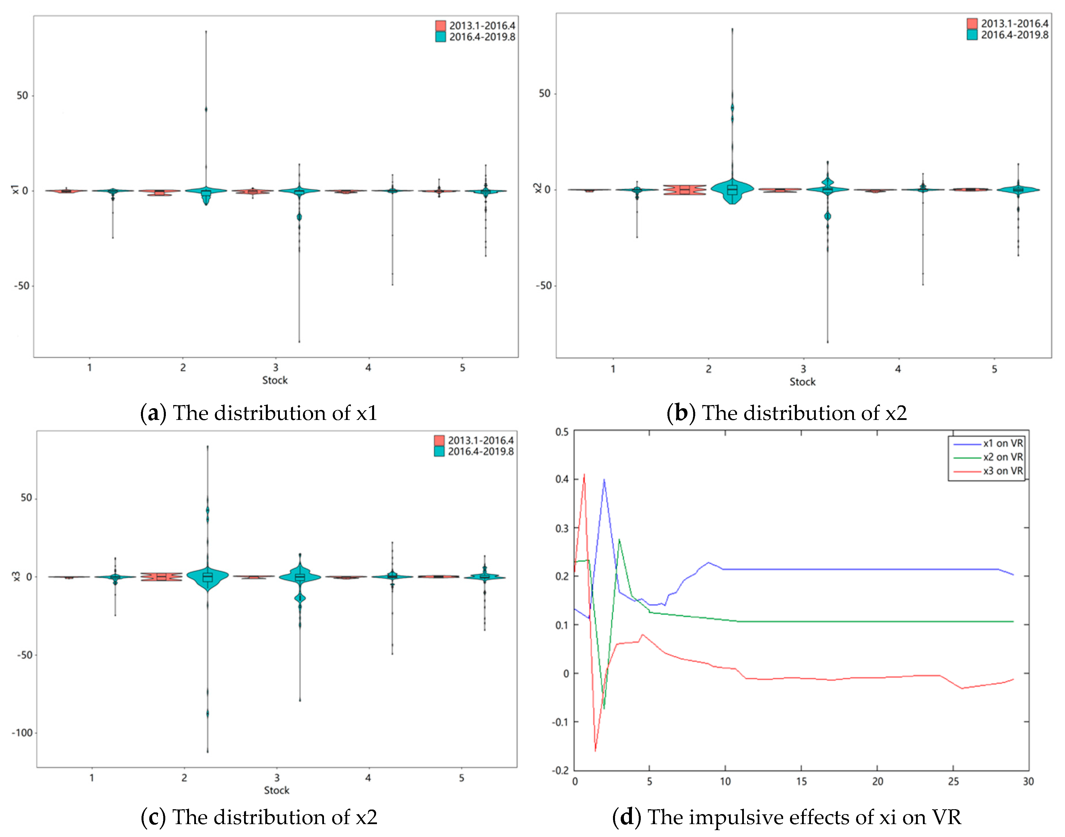
Step 6. Put the revised estimation into Kalman Filtering to continue the next round of iteration, until convergence. Based on the results, some features of cognitive biases are shown in Figure 1, Figure 2 and Figure 3. Additionally, the estimation results are shown as follows:
Step 7. Calculate the 5-day and 12-day EMACB based on the previous measurement outcomes.
Step 8. Construct the EV model for the risk seeker and calculate the objective weights of each stock.
Step 9. Construct the EV model for the risk averter and obtain the weights allocation. The results of step 8 and 9 are expressed in Table 7.
Figure 1a–c reveal the distributions of the chosen stocks’ collective cognitive bias (x1, x2, x3). These distributions are acquired by a series of data that originated from two periods. What can be found in the figures is that the possible value range of three cognitive biases in the second time period are much broader than the first period. The features shown in the picture support the fact that the increasing volume of information in the economic environment does interfere with judgment, and leads to more severe cognition bias.
In Figure 1d, the stock trading volume ratio varies with the changes of the cognitive bias in a short period. Sudden changes in cognitive bias can lead to violent trading swings. In the long run, the equilibrium price is determined by the asset value, which is not affected by short-term cognition. Besides, the red curve has the strongest impulsive effects among the three curves, which indicates the VR (volume ratio) is more sensitive to anchoring values.
It is obvious in Table 7 that the risk averter tends to give more evenly weights for each chosen stock, which is different from the risk seeker. In other words, the risk averter has stronger demand to diversify risk in the investment prediction of September, 2019. However, the results only represent the investment features in one month with a 5-stock portfolio. Whether the proposed method has value in general applications still need to be verified in Section 4.
4. Discussion
In order to discuss the general applicability of the EV method, we suggest demonstratation from the following aspects.
4.1. General Validation of the Example
To avoid the chance of the previous results, we decided to expand the size of the sample data, which was collected from January, 2000 to August, 2019. After stripping out the stocks with significantly incomplete data, we selected 100 stocks from 44 major sectors SHCI (Shanghai Securities Composite Index) as experimental samples. The general validation experiments are as follows.
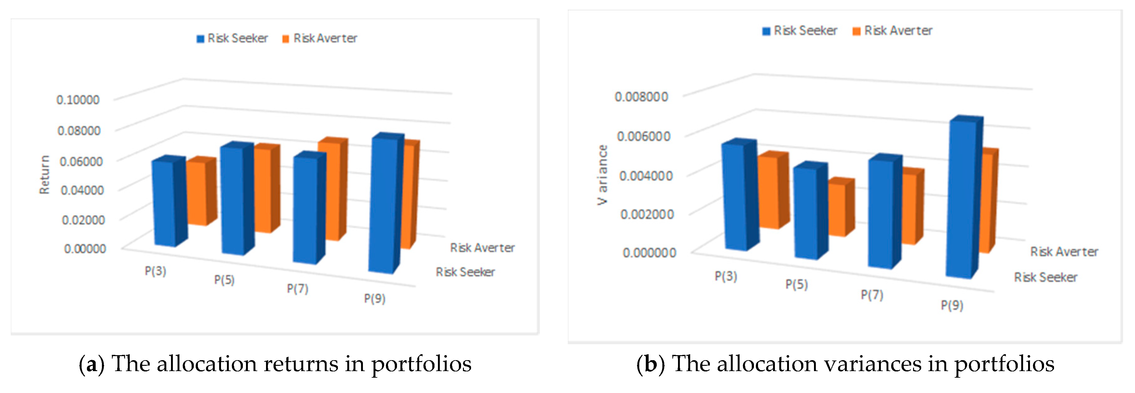
(1) Changes in the number of stocks
First, it has to be validated whether the number of stocks in a portfolio could impact the initial results. We identified the decision heterogeneity between two kinds of investor in the previous 5-stock portfolio. However, what will happen if the number of stocks in a portfolio changes? To acquire convincing results, we randomly extracted stocks from the experimental sample base as candidates for the experiment. These candidates cannot come from the same sector and show no correlation in the Pearson tests. The relevant results are shown in Figure 2.
In Figure 2, the allocation results of two kinds of investors are presented under the premise of the 3/5/7/9 stock in a portfolio. (P (j) represents there are j stocks in a portfolio, j = 3,5,7,9. Most of the results show that the risk seeker obtains higher returns, while the risk averter undertakes less risks in the investment, except group P (7), without a significant difference in returns. After comparison, more than 75% of the results are consistent with the previous results.
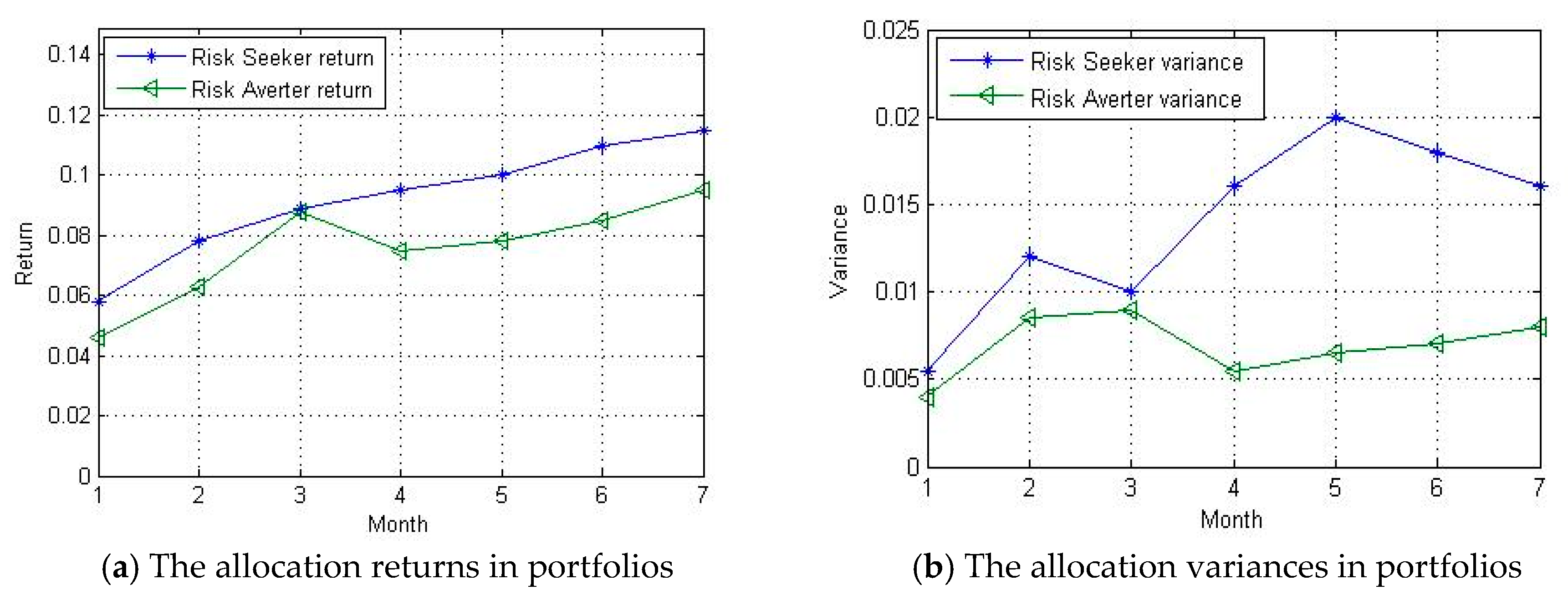
(2) Changes in the experimental periods
Meanwhile, the results can also be influenced by the experimental periods. The initial results in one month can hardly reveal the true features with the appliance of the EV method. As such, the above example in Section 3.2 should be put in different periods (1 month, 2 months, …, 7 months) to verify whether the proposed method creates a contingency to some extent. The allocation weights acquired from the EV method will be updated based on the existing data. The corresponding results are reflected in Figure 3.
According to Figure 3, we can tell that the gap between two investors’ returns seems small in the first three periods, and becomes much bigger in the last four periods. While in Figure 3b, the variances of the risk seeker have a larger fluctuation and are always higher than the risk averter’s. Additionally, there is no evidence to suggest that the risk averter could gain more returns than the risk seeker with a stable variance. Based on the comparison analysis, the results are consistent with the initial one.
4.2. Performance Comparison of Different Methods
Besides the general validation of the example, the efficiency of the proposed method needs to be testified by the comparison of similar methods as well. We respectively calculated the allocation results through different methods (e.g., the EV method, the existing MV method, and two improved MV methods mentioned by Dai et al. [63]), and the performance comparison is shown in Table 8.
In Table 8, the efficiency of these methods is compared from the aspects of return, variance, turnover, and sharp ratio, respectively. In terms of return, the portfolio obtained from the EV method performs much better than the other three, while there is no obvious difference between the returns of the MVSRB method and the MVSRE method.
When talking about variance, it has long been regarded as the indicator of risk. In Table 8, for the risk seeker, he gains a big pay-off from the EV method portfolio with a lower risk compared to the others. For the risk averter, the variance from the MVSRE method seems less than that from the EV method but not that much.
The turnover refers to the average monthly trading volume. In consideration of the transaction costs, a high turnover will offset the achievements of portfolios. In Table 8, the turnover rates of the portfolio in the EV method are relatively low in comparison, which means the transaction costs from the EV method are under control, though not the lowest.
In the end, we chose to calculate the sharp ratio (SR) to evaluate the effective gains after removing the risk. As is in Table 8, the EV method shows big advantages in investment achievement, which demonstrates its efficiency in applications. Based on the performances shown above, the EV method is suitable to be applied in the investment decision-making process.
Compared to the improved MV methods, the defect of the MV method is that the mean value cannot effectively represent the expected return. For one, the mean value is weak in reflecting irregular fluctuations of stock prices. For another, the mean value does not show investors’ expectations, so that it cannot be used as an effective boundary constraint under the target of minimum risk. The construction of the EV method can exactly remedy these drawbacks.
5. Conclusions
This paper proposed the measurement method of collective cognitive bias and improved the MV method to solve the problem of stock allocation. The primary contributions of this study are summarized as follows: (1) Based on the formation mechanism of collective cognitive bias, a state-space method with a hybrid algorithm was proposed to measure the cognitive biases; (2) given the importance of the collective cognitive bias in return prediction, EMACB-V was constructed to evaluate the expected return in stock allocation; and (3) considering the difference of investors’ risk preferences, a symmetric investment method was put forward to obtain the heterogeneous stock allocation.
However, there are still some limitations in the application of this method. The proposed method is suitable for stock investment, but the impact of cognitive bias on other investment situations was not investigated. In addition, in this research, the authors are more inclined to understand the cognitive states of Chinese investors, and it is unclear sure whether the investors in other countries have equal sensitivities to these stimulus factors. In the future, we will highlight the following directions. First, stock portfolios were regarded as the main research objects in this paper. In practical applications, however, investors must be challenged by composite portfolios, including bonds, stocks, funds, options, etc. Therefore, an investment method with diversified capital should be improved in the future work. Second, this method is more available for short-term investments. Thus, a dynamic investment allocation accompanied with a subjective environment should be established in the long run.
Author Contributions
Conceptualization, L.W. and H.W.; methodology, L.W.; software, G.L. and W.L.; validation, L.W., H.W. and G.L.; formal analysis, L.W. and W.L.; investigation, L.W. and W.L.; resources, L.W.; data curation, L.W. and W.L.; writing—original draft preparation, L.W.; writing—review and editing, G.L.; supervision, H.W.; funding acquisition, G.L. All authors have read and agreed to the published version of the manuscript.
Funding
This research was funded by Hebei Municipal Natural Science Foundation (Grant No. G2019501105).
Conflicts of Interest
The authors declare no conflict of interest.
References
- Sharpe, W.F. Asset allocation: Management style and performance measurement. J. Portf. Manag. 1992, 18, 7–19. [Google Scholar] [CrossRef]
- Yam, S.C.P.; Yang, H.; Yuen, F.L. Optimal asset allocation: Risk and information uncertainty. Eur. J. Oper. Res. 2016, 251, 554–561. [Google Scholar] [CrossRef] [Green Version]
- Meucci, A. Evaluating allocation. In Risk and Asset Allocation, 2nd ed.; Avellaneda, M., Barone-Adeisi, G., Broadie, M., Davis, M.H.A., et al., Eds.; Springer: New York, NY, USA, 2005; Volume 6, pp. 1–532. [Google Scholar]
- Hong, H.; Stein, J. A unified theory of under reaction momentum trading, and overreaction in asset markets. J. Financ. 1999, 54, 2143–2184. [Google Scholar] [CrossRef] [Green Version]
- Chan, W.S.; Frankel, R.; Kothari, S.P. Testing behavioral finance theories using trends and consistency in financial performance. J. Account. Econ. 2004, 38, 3–50. [Google Scholar] [CrossRef]
- Mazumdar, T.; Raj, S.P.; Sinha, I. Reference price research: Review and propositions. J. Mark. 2005, 69, 84–102. [Google Scholar] [CrossRef]
- Völckner, F. The dual role of price: Decomposing consumers’ reactions to price. J. Acad. Mark. Sci. 2008, 36, 359–377. [Google Scholar] [CrossRef]
- Bauer, R.; Cosemans, M.; Schotman, P.C. Conditional asset pricing and stock market anomalies in Europe. Eur. Financ. Manag. 2010, 16, 165–190. [Google Scholar] [CrossRef]
- Vanhuele, M.; Drèze, X. Measuring the price knowledge shoppers bring to the store. J. Mark. 2002, 66, 72–85. [Google Scholar] [CrossRef] [Green Version]
- Zielke, S. How price image dimensions influence shopping intentions for different store formats. Eur. J. Mark. 2010, 44, 748–770. [Google Scholar] [CrossRef]
- Ball, R.; Kothari, S.P.; Shanken, J. Problems in measuring portfolio performance: An application to contrarian investment strategies. J. Financ. Econ. 1995, 38, 79–107. [Google Scholar] [CrossRef]
- Coval, J.; Shumway, T. Do behavioural biases affect prices. J. Financ. 2005, 60, 1–34. [Google Scholar] [CrossRef] [Green Version]
- Daniel, K.D.; Hirshleifer, D.; Subrahmanyam, A. Investor psychology and security market under- and overreactions. J. Financ. 1998, 53, 1839–1885. [Google Scholar] [CrossRef] [Green Version]
- De Bondt, W.; Thaler, R. Does the stock market overreact. J. Financ. 1985, 40, 793–805. [Google Scholar] [CrossRef]
- Hou, K.; Xue, C.; Zhang, L. Digesting anomalies: An investment approach. Rev. Financ. Stud. 2015, 28, 650–705. [Google Scholar] [CrossRef] [Green Version]
- Subrahmanyam, A. Behavioral finance: A review and synthesis. Eur. Financ. Manag. 2007, 14, 12–29. [Google Scholar] [CrossRef]
- Banholzer, N.; Heiden, S.; Schneller, D. Exploiting investor sentiment for portfolio optimization. Bus. Res. 2018, 12, 671–702. [Google Scholar] [CrossRef] [Green Version]
- Kariofyllas, S.; Philippas, D.; Siriopoulos, C. Cognitive biases in investors’ behaviour under stress: Evidence from the london stock exchange. Int. Rev. Financ. Anal. 2017, 54, 54–62. [Google Scholar] [CrossRef]
- Antoniou, C.; Doukas, J.A.; Subrahmanyam, A. Cognitive dissonance, sentiment and momentum. J. Financ. Quant. Anal. 2013, 48, 245–275. [Google Scholar] [CrossRef] [Green Version]
- Goetzmann, W.N.; Zhu, N. Rain or shine: Where is the weather effect. Eur. Financ. Manag. 2005, 11, 559–578. [Google Scholar] [CrossRef]
- Baker, M.; Wurgler, J. Investor sentiment in the stock market. J. Econ. Perspect. 2007, 21, 129–151. [Google Scholar] [CrossRef] [Green Version]
- Baker, M.; Wurgler, J. Investor sentiment and the cross-section of stock returns. J. Financ. 2006, 4, 1645–1680. [Google Scholar] [CrossRef] [Green Version]
- Brown, G.W.; Cliff, M.T. Investor sentiment and asset valuation. J. Bus. 2005, 78, 405–440. [Google Scholar] [CrossRef]
- Wattanacharoensil, W.; Laornual, D. A systematic review of cognitive biases in tourist decisions. Tour. Manag. 2019, 75, 353–369. [Google Scholar] [CrossRef]
- Jesse, M.P.; Andrew, S. Cognitive baises in emergency physicians: A pilot study. J. Emerg. Med. 2019, 57, 168–172. [Google Scholar] [CrossRef]
- Barberis, N.; Shleifer, A.; Vishny, R.W. A model of investor sentiment. J. Financ. Econ. 1998, 49, 307–343. [Google Scholar] [CrossRef]
- Bollen, J.; Mao, H.; Zeng, X. Twitter mood predicts the stock market. J. Comput. Sci. 2011, 2, 1–8. [Google Scholar] [CrossRef] [Green Version]
- Tversky, A.; Kahneman, D. Judgement under uncertainty: Heuristics and biases. Science 1974, 185, 1124–1131. [Google Scholar] [CrossRef]
- Shefrin, H.; Stateman, M. The disposition to sell winners too early and ride losers too long: Theory and evidence. J. Financ. 1985, 40, 777–790. [Google Scholar] [CrossRef]
- Duclos, R. The psychology of investment behavior: Biasing financial decision-making one graph at a time. J. Consum. Psychol. 2015, 25, 317–325. [Google Scholar] [CrossRef]
- Tversky, A.; Kahneman, D. Availability: A heuristic for judging frequency and probability. Cogn. Psychol. 1973, 5, 207–232. [Google Scholar] [CrossRef]
- Kumar, S.; Goyal, N. Behavioural biases in investment decision making—A systematic literature review. Qual. Res. Financ. Mark. 2015, 7, 88–108. [Google Scholar] [CrossRef]
- Statman, M.; Thorley, S.; Vorkink, K. Investor overconfidence and trading volume. Rev. Financ. Stud. 2006, 19, 1531–1565. [Google Scholar] [CrossRef]
- Seasholes, M.S.; Zhu, N. Individual investors and local bias. J. Financ. 2010, 65, 1987–2010. [Google Scholar] [CrossRef]
- Corcoran, C.M. Long/Short Market Dynamics: Trading Strategies for Today’s Markets, 3rd ed.; John Wiley & Sons Ltd: West Sussex, UK, 2007; pp. 1–358. [Google Scholar]
- Kandel, S.; Stambaugh, R.F. On the predictability of stock returns: An asset-allocation perspective. J. Financ. 1996, 51, 385–424. [Google Scholar] [CrossRef]
- Marston, R.C. Portfolio Design: A Modern Approach to Asset Allocation, 7th ed.; John Wiley & Sons Ltd.: Hoboken, NJ, USA, 2011; pp. 1–337. [Google Scholar]
- Sharpe, W.F. Capital asset prices: A theory of market equilibrium under conditions of risk. J. Financ. 1964, 19, 425–442. [Google Scholar] [CrossRef]
- Sharpe, W.F. A simplified model for portfolio analysis. Manag. Sci. 1963, 9, 277–293. [Google Scholar] [CrossRef] [Green Version]
- Mao, J.C.T. Models of capital budgeting, E-V vs E-S. J. Financ. Quant. Anal. 1970, 4, 657–675. [Google Scholar] [CrossRef]
- Konno, H.; Yamazaki, H. Mean-absolute deviation portfolio optimization model and its applications to Tokyo stock market. Manag. Sci. 1991, 37, 519–531. [Google Scholar] [CrossRef] [Green Version]
- Feinstein, C.D.; Thapa, M.N. Notes: A reformulation of a mean-absolute deviation portfolio optimization model. Manag. Sci. 1993, 39, 1552–1553. [Google Scholar] [CrossRef]
- Dowd, K. Beyond Value at Risk: The New Science of Risk Management, 8th ed.; John Wiley & Sons Ltd.: London, UK, 1998; pp. 1–288. [Google Scholar]
- Jorion, P. Value at Risk: The New Benchmark for Controlling Market Risk, 2nd ed.; Irwin: Chicago, IL, USA, 1997; pp. 1–544. [Google Scholar]
- Young, M.R. A minimax portfolio selection rule with linear programming solution. Manag. Sci. 1998, 44, 673–683. [Google Scholar] [CrossRef] [Green Version]
- Guijarro, F. A similarity measure for the cardinality constrained frontier in the mean–variance optimization model. J. Oper. Res. Soc. 2017, 69, 928–945. [Google Scholar] [CrossRef]
- Qin, Z.; Kar, S.; Zheng, H. Uncertain portfolio adjusting model using semiabsolute deviation. Soft Comput. 2014, 20, 717–725. [Google Scholar] [CrossRef]
- Kalayci, C.B.; Ertenlice, O.; Akbay, M.A. A comprehensive review of deterministic models and applications for mean-variance portfolio optimization. Expert Syst. Appl. 2019, 125, 345–368. [Google Scholar] [CrossRef]
- Alexander, G. Short selling and efficient sets. J. Financ. 1993, 48, 1497–1506. [Google Scholar] [CrossRef]
- Athanasios, A.P. Dynamic risk management of the lending rate policy of an interacted portfolio of loans via an investment strategy into a discrete stochastic framework. Econ. Modeling 2008, 25, 658–675. [Google Scholar] [CrossRef]
- Eichner, T.; Wagener, A. Tempering effects of (dependent) background risks: A mean-variance analysis of portfolio selection. J. Math. Econ. 2012, 48, 422–430. [Google Scholar] [CrossRef]
- Lopes, L. Between hope and fear: The psychology of risk. Adv. Exp. Soc. Psychol. 1987, 20, 255–295. [Google Scholar] [CrossRef]
- Shefrin, H.; Statman, M. Behavioral portfolio theory. J. Financ. Quant. Anal. 2000, 35, 127–151. [Google Scholar] [CrossRef] [Green Version]
- Roy, A.D. Safety-first and the holding of assets. Econometrics 1952, 20, 431–449. [Google Scholar] [CrossRef]
- Markowitz, H. Portfolio selection. J. Financ. 1952, 7, 77–91. [Google Scholar]
- Statman, M.; Woods, V. Investment temperament. J. Invest. Consult. 2004, 7, 55–66. [Google Scholar]
- Kondor, I.; Pafka, S.; Nagy, G. Noise sensitivity of portfolio selection under various risk measures. J. Bank. Financ. 2007, 31, 1545–1573. [Google Scholar] [CrossRef] [Green Version]
- Yang, C.P.; Xie, J. Sentiment perceived portfolio optimization. J. Converg. Inf. Technol. 2011, 6, 203–209. [Google Scholar]
- Boyle, P.; Garlappi, L.; Uppal, R.; Wang, T. Keynes meets Markowitz: The tradeoff between familiarity and diversification. Manag. Sci. 2012, 58, 253–272. [Google Scholar] [CrossRef] [Green Version]
- Das, S.; Markowitz, H.; Scheid, J.; Statman, M. Portfolio optimization with mental accounts. J. Financ. Quant. Anal. 2010, 45, 311–334. [Google Scholar] [CrossRef] [Green Version]
- Wickham, P.A. The representativeness heuristic in judgements involving entrepreneurial success and failure. Manag. Decis. 2003, 41, 156–167. [Google Scholar] [CrossRef]
- Huang, A.G.; Wirjanto, T.S. Is China’s P/E ratio too low? Examining the role of earnings volatility. Pac. Basin Financ. J. 2012, 20, 41–61. [Google Scholar] [CrossRef]
- Dai, Z.; Wang, F. Sparse and robust mean-variance portfolio optimization problems. Phys. A 2019, 523, 1371–1378. [Google Scholar] [CrossRef]
Figure 1.
Some characteristics of cognitive biases.

Figure 2.
The allocation results in different numbers of stocks in a portfolio.

Figure 3.
The allocation results in different periods.


Table 1.
The selection basis of the stimulus factor.
| Basis | Meaning | Stimulus Factor |
|---|---|---|
| Representativeness | A person following representativeness prefers to evaluate uncertain events through the features in the similar events. | Industry Sector Index |
| Availability | Availability refers to the situation in which people assess events by the ease with the accessible influence. | PE (Price/Earning) |
| Anchoring | Anchoring refers to the situation in which people consider the initial feature as the key factor of decision. | EMA (5) |
Table 2.
Variable description.
| Symbol | Variable | Meaning |
|---|---|---|
| VR | Volume Ratio | VR = trading volume in current period/5-day weighted average trading volume. |
| I1 | Industry Sector Index | This index reflects the composite stock price changes in corresponding industry sectors. |
| I2 | PE | PE = Price per shar/Earnings per share. |
| I3 | EMA (5) | EMA (5) refers to a 5-day weighted average price of exponential decays. |
Table 3.
Descriptive statistics.
| S1 | S2 | S3 | S4 | S5 | |
|---|---|---|---|---|---|
| observation | 1706 | 1658 | 1700 | 1687 | 1711 |
| mean | 87.4734 | 101.3718 | 428.1459 | 419.2882 | 22.7761 |
| median | 87.6000 | 103.1450 | 417.8950 | 411.8350 | 21.0800 |
| std. dev. | 69.4728 | 7.7212 | 6.9736 | 5.9473 | 6.5866 |
| min | 13.1300 | 94.4700 | 377.7600 | 383.4900 | 18.3300 |
| max | 157.4400 | 137.0000 | 445.9900 | 426.1600 | 35.8000 |
Table 4.
Pearson correlation test.
| S1 | S2 | S3 | S4 | S5 | |
|---|---|---|---|---|---|
| S1 | 1 | ||||
| S2 | 0.0574 | 1 | |||
| S3 | 0.1257 | 0.0302 | 1 | ||
| S4 | 0.0844 | 0.0717 | 0.2047 | 1 | |
| S5 | 0.1024 | 0.2092 | 0.1615 | 0.2286 | 1 |
Table 5.
The Augmented Dickey-Fuller (ADF) test.
| Variable | ADF Test | ||
|---|---|---|---|
| T-Statistics | Prob. | Stability | |
| dVR | −9.866843 | 0.0000 | stable *** |
| dLI1 | −6.634674 | 0.0000 | stable *** |
| dLI2 | −7.906096 | 0.0000 | stable *** |
| dLI3 | −3.473008 | 0.0007 | stable *** |
*** After one time difference, the data of each variable are stationary sequences at the significance level of 1%.
Table 6.
Johansen co-integration test.
| Hypothesized No. of CE(s) | Eigenvalue | Trace Test | Max-Eigen | ||
|---|---|---|---|---|---|
| Statistic | Prob. ** | Statistic | Prob. ** | ||
| None * | 0.577532 | 203.5052 | 0.0012 | 55.02875 | 0.0009 |
| At most 1 * | 0.480721 | 104.7045 | 0.0000 | 26.11564 | 0.0140 |
| At most 2 * | 0.421976 | 37.17026 | 0.0000 | 40.2293 | 0.0007 |
| At most 3 * | 0.320903 | 63.28152 | 0.0001 | 19.94836 | 0.0109 |
| At most 4 * | 0.151025 | 17.22287 | 0.0000 | 17.22289 | 0.0013 |
1 “*” represents rejection of the null hypothesis at the 95% significance level; “**” indicates the p-value in MacKinnon and Huang and Michelis (1999). At the significance level of 5%, there is a co-integration relationship between the variables, which means a long-term equilibrium relationship exists between them.
Table 7.
Stock allocation for a heterogeneous investor.
| Type | Weights Allocation | Stock Investment Ratio | ||||
|---|---|---|---|---|---|---|
| S1 | S2 | S3 | S4 | S5 | ||
| InvestorSK | 0.477 | 0.146 | 0.195 | 0.093 | 0.088 | 70% |
| InvestorAV | 0.295 | 0.204 | 0.231 | 0.143 | 0.127 | 30% |
Table 8.
Methods of the performance comparison.
| Client Type | Investor-sk | Investor-av | Investor-sk | Investor-av | |||||
|---|---|---|---|---|---|---|---|---|---|
| Time Span | Return | Variance | Return | Variance | Turnover | Sharp Ratio | Turnover | Sharp Ratio | |
| EV: 1 month | 0.05814 | 0.005494 | 0.04646 | 0.003990 | 0.3698 | 0.4452 | 0.4514 | 0.4398 | |
| 2 months | 0.07849 | 0.012097 | 0.06361 | 0.008504 | 0.5167 | 0.3257 | 0.5759 | 0.3261 | |
| 3 months | 0.08956 | 0.010745 | 0.08874 | 0.009003 | 0.5384 | 0.3364 | 0.5578 | 0.3349 | |
| 5 months | 0.10430 | 0.024130 | 0.07963 | 0.006521 | 0.6272 | 0.2681 | 0.6379 | 0.2705 | |
| 7 months | 0.11309 | 0.016732 | 0.09588 | 0.008136 | 0.6425 | 0.4342 | 0.7100 | 0.4317 | |
| MV: 1 month | 0.05575 | 0.005508 | 0.04313 | 0.009940 | 0.4658 | 0.3089 | 0.4776 | 0.3073 | |
| 2 months | 0.06953 | 0.011986 | 0.05968 | 0.010730 | 0.5783 | 0.2670 | 0.5841 | 0.2660 | |
| 3 months | 0.07377 | 0.010800 | 0.09040 | 0.010340 | 0.6420 | 0.2683 | 0.6469 | 0.2676 | |
| 5 months | 0.08841 | 0.034759 | 0.08006 | 0.011406 | 0.6617 | 0.1875 | 0.6672 | 0.1884 | |
| 7 months | 0.08350 | 0.021804 | 0.07833 | 0.014035 | 0.7125 | 0.2966 | 0.7148 | 0.2948 | |
| MVSRB: 1 month | 0.05640 | 0.005507 | 0.04450 | 0.008128 | 0.4463 | 0.4286 | 0.4508 | 0.4185 | |
| 2 months | 0.07788 | 0.012189 | 0.06117 | 0.009635 | 0.5551 | 0.2968 | 0.5575 | 0.3011 | |
| 3 months | 0.08007 | 0.010796 | 0.08817 | 0.010131 | 0.5447 | 0.3204 | 0.5485 | 0.3192 | |
| 5 months | 0.09892 | 0.025488 | 0.08001 | 0.009809 | 0.6314 | 0.2555 | 0.6356 | 0.2560 | |
| 7 months | 0.09733 | 0.017329 | 0.08727 | 0.012523 | 0.7071 | 0.3987 | 0.7132 | 0.3976 | |
| MVSRE: 1 month | 0.05603 | 0.005504 | 0.04374 | 0.003984 | 0.3012 | 0.3839 | 0.4670 | 0.3801 | |
| 2 months | 0.07840 | 0.011995 | 0.06159 | 0.008498 | 0.4573 | 0.2789 | 0.5820 | 0.2794 | |
| 3 months | 0.07994 | 0.010787 | 0.08723 | 0.009003 | 0.5218 | 0.3029 | 0.6224 | 0.3018 | |
| 5 months | 0.10050 | 0.033625 | 0.07977 | 0.006511 | 0.5344 | 0.2417 | 0.6472 | 0.2435 | |
| 7 months | 0.09853 | 0.016923 | 0.08589 | 0.008127 | 0.5961 | 0.3213 | 0.7076 | 0.7092 | |
| Return Comparison: | EVSK ≻ MVSRESK ≻ MVSRBSK ≻ MVSK; EVAV ≻ MVSRBAV ≻ MVSREAV ≻ MVAV | ||||||||
| Risk Comparison: | MVSK ≻ MVSRBSK ≻ MVSRESK ≻ EVSK; MVAV ≻ MVSRBAV ≻ EVAV ≻ MVSREAV | ||||||||
| Turnover Comparison: | MVSK ≻ MVSRBSK ≻ EVSK ≻ MVSRESK; MVAV ≻ MVSREAV ≻ EVAV ≻ MVSRBAV | ||||||||
| SR Comparison: | EVSK ≻ MVSRBSK ≻ MASRESK ≻ MVSK; EVAV ≻ MVSRBAV ≻ MASREAV ≻ MVAV | ||||||||
© 2020 by the authors. Licensee MDPI, Basel, Switzerland. This article is an open access article distributed under the terms and conditions of the Creative Commons Attribution (CC BY) license (http://creativecommons.org/licenses/by/4.0/).
Share and Cite
MDPI and ACS Style
Wang, L.; Wu, H.; Li, G.; Lu, W. An Improved MV Method for Stock Allocation Based on the State-Space Measure of Cognitive Bias with a Hybrid Algorithm. Symmetry 2020, 12, 1036. https://0-doi-org.brum.beds.ac.uk/10.3390/sym12061036
AMA Style
Wang L, Wu H, Li G, Lu W. An Improved MV Method for Stock Allocation Based on the State-Space Measure of Cognitive Bias with a Hybrid Algorithm. Symmetry. 2020; 12(6):1036. https://0-doi-org.brum.beds.ac.uk/10.3390/sym12061036
Chicago/Turabian StyleWang, Liwen, Hecheng Wu, Gang Li, and Weixue Lu. 2020. "An Improved MV Method for Stock Allocation Based on the State-Space Measure of Cognitive Bias with a Hybrid Algorithm" Symmetry 12, no. 6: 1036. https://0-doi-org.brum.beds.ac.uk/10.3390/sym12061036
Note that from the first issue of 2016, this journal uses article numbers instead of page numbers. See further details here.