Advanced Algorithms and Common Solutions to Variational Inequalities


1
Department of Mathematics, Sohag University, Sohag 82524, Egypt
2
Department of Mathematics, King Mongkut’s University of Technology Thonburi (KMUTT), Bangkok 10140, Thailand
3
Institute of Research and Development of Processes IIDP, University of the Basque Country, 48940 Leioa, Spain
*
Author to whom correspondence should be addressed.
Symmetry 2020, 12(7), 1198; https://0-doi-org.brum.beds.ac.uk/10.3390/sym12071198
Submission received: 30 June 2020
/
Revised: 16 July 2020
/
Accepted: 17 July 2020
/
Published: 20 July 2020
(This article belongs to the Special Issue Iterative Numerical Functional Analysis with Applications)
Abstract
:The paper aims to present advanced algorithms arising out of adding the inertial technical and shrinking projection terms to ordinary parallel and cyclic hybrid inertial sub-gradient extra-gradient algorithms (for short, PCHISE). Via these algorithms, common solutions of variational inequality problems (CSVIP) and strong convergence results are obtained in Hilbert spaces. The structure of this problem is to find a solution to a system of unrelated VI fronting for set-valued mappings. To clarify the acceleration, effectiveness, and performance of our parallel and cyclic algorithms, numerical contributions have been incorporated. In this direction, our results unify and generalize some related papers in the literature.
1. Introduction
In this manuscript, we discuss the problem of finding fixed points which also solve VI via a Hilbert space (Hs). Let ¥ be a nonempty closed convex subset (ccs) of Hs ℸ under the induced norm and the inner product
The structure of the variational inequality problem (VIP) was built by the authors [1], for finding such that
where be a nonlinear mapping. They refer to the set of solutions of VIP (1) as .
VI is involved in many interesting fields like, transportation, economics, engineering mechanics, mathematical programming. It is considered an indispensable tool in such specializations (see, for example, [2,3,4,5,6,7,8]). VI widely spread in optimization problems (OPs), where the algorithms were used solving it, see [7,9].
Under suitable stipulation to talk VIPs there is a two-way: projection modes and regularized manners. According to these lines, many iterative schemes have been presented and discuss for solving VIPs. Here, We focused on the first type. One of the easiest ways is using the gradient projection method, because when calculating it only needs one projection on the feasible set. However, the convergence of this method requires slightly strong assumptions that operators are strongly monotone or inverse strongly monotone. Via Lipschitz continuous and monotone mappings ℷ for solving saddle point problems and generalizing VIPs. Another projection method called the extra-gradient method has been presented by Korpelevich [10], which is built as below:
for a suitable parameter ℓ and the metric projection onto ¥. Finding a projection and simplicity of the method depend on ¥ if it simple the extra-gradient method is computable and very useful otherwise the extra-gradient method is more complicated. The extra-gradient method used to solve two distance OPs if ¥ is a cc set.
In a Hs, the weak convergence of a solution of the VIPs is incorporated under the sub-gradient extra-gradient method [11] by the below algorithm:
where is a half-space defined as follows:
Authors [12] accelerate the speed of convergence of the algorithm by building the following algorithm:
Our paper is interested in finding CSVIP. The CSVIP here is to find a point such that
where be a nonlinear mapping and be a finite family of non-empty ccs of ℸ such that Please note that If CSVIP (2) reduce to VIP (1). Here CSVIPs takes many forms such as: Convex feasibility problem (CFP), if we consider all , then we find a point in the non-empty intersection of a finite family of cc sets. Common fixed point problem (CFPP) If we take the sets are the fixed point sets in (CFP). These problems have been studied in-depth and expansion, and their numerous applications have become the focus of attention of many researchers see [13,14,15,16,17,18,19].
For multi-valued mappings of , an algorithm for solving the CSVIP is given by [20]. For simplicity we list the below algorithm for is a single-valued: Choose and compute
the approximation of the algorithm (3), can be found by constructing subsets ,.., and and solve the following minimization problem:
when N is large, this task can be very costly. Respect to the power of the number of half-spaces, the number of subcases in the explicit solution formula of the problem (4) is two.
In Banach spaces, for finding a common element of the set of fixed points via a family of asymptotically quasi non-expansive mappings the authors [21,22] derived two strongly convergent parallel hybrid iterative methods. This algorithm can be formulated in Hilbert spaces as follows:
where According to this algorithm, the approximation is defined as the projection of onto , and finding the explicit form of the sets and perform numerical experiments seems complicated. By the same scenario, Hieu [23], introduced two PCHSE algorithms for CSVIPs in Hilbert spaces and analyze their convergence by numerical results.
Our main goal in this paper is to present iterative procedures for solving CSVIPs and prove its strong convergence. We called it, PCHISE algorithms. Our algorithms generates a sequence that converges strongly to the nearest point projection of the starting point onto the solution set of the CSVIP. To simplify this convergence, we use the inertial technical and shrinking projection methods. Also, some numerical experiments to support our results are given.
The outline of this work is as follows: In the next section, we give a definition and lemmas that we will use in study of the strong convergence analysis. Strong convergence results are obtained bu these procedures in Section 3, and at the ending, in Section 4, non-trivial two computational examples to discuss the performance of our algorithms and support theoretical results are incorporated.
2. Definition and Necessary Lemmas
In this section, we recall some definitions and results which will be used later.
Definition 1.
[24] For all a nonlinear operator ℷ is called
- (i)
- monotone if
- (ii)
- pseudomonotone if leads to
- (iii)
- inverse strongly monotone (ism) if there exists such that
- (iv)
- maximal monotone if it is monotone and its graphis not a proper subset of one of any other monotone mapping,
- (v)
- L-Lipschitz continuous if there exists a positive constant L such that
- (vi)
- nonexpansive ifHere, the set is referred to the set of all fixed points of a mapping ℷ.
It’s obvious that a monotone mapping is maximal iff, for each such that for all , it follows that .
For each , the projection defined by . Also, exists and is unique because is nonempty ccs of ℸ. The projection has the following properties:
Lemma 2.
[24] Assume that is a projection. Then
(i) is 1-ism, i.e., for each ,
(ii) For all ℘⅁
(iii) if and only if
Lemma 3.
[25] Suppose that ℷ is a monotone, hemi-continuous mapping form onto ℸ, where ¥ is a non-empty ccs of a Hs ℸ, then
Lemma 4.
[26] Suppose that is a ccs of a Hs ℸ. Given that and the set
is cc.
The normal cone to a set at a point defined by
Thus, the following result is very important.
Lemma 5.
[27] Suppose that ℷ is a monotone, hemi-continuous mapping form ¥ onto ℸ, where ¥ is a non-empty ccs of a Hs ℸ, with Let ℑ be a mapping defined by
Then ℑ is a maximal monotone and ℑ
3. Main Theorems
This part is devoted to discuss the strong converges for our proposed algorithms under the following considerations: The collection is Lipschitz continuous with the same constant L. Via , is also L-Lipschitz continuous for each . Finally, we consider is non-empty.
Theorem 1.
(PHISE algorithm)
Assume that ℸ is a rHs and , where be ccs of ℸ. Let be a finite collection of monotone and L-Lipschitz continuous mappings and the solution set Θ is nonempty. Let be a sequence generated by , for all and
where and Assume that Then the sequence converges strongly to
Proof.
The proof is divided into the below steps
Step 1. Show that
where and
Let then by Lemma 1 (i), we can write
Also, by simple calculations, we can find
Similarly,
Since, is monotone on and , we can get
This together with yields
So
From definition of the metric projection onto , one can obtain
Thus, by (10), we get
Put and write again From Lemma 2 (ii) and (9), one can write
From (11), we have
Hence, we have the inequality (6).
Step 2. Show that is well-defined for all and Since is Lipschitz continuous, thus, Lemma 3 confirm that is too for all . Hence, is closed and convex. It follows from the definition of and Lemma 4 that, is closed and convex for each
Let thus we obtain from Step 1 that
Therefore, we have Thus, and is will-defined.
Step 3. Prove that exists. Since is ccs of then there is a unique such that
From and we can get
On the other hand, as we have
This proves that is bounded and non-decreasing. Hence, exists.
Step 4. Prove that for all , the following relation holds
From and we can get
For this inequality, letting and using Step 3, we find
Since , then we have
From (15) and the definitions of , , we have
as for all By triangle inequality and using (15) and (17), one can obtain that
as for all From Step 1 and the triangle inequality, for each one has
Step 5. Show that the strongly convergent of and generated by (5) to . Let has a weak cluster point , and has a subsequence converging weakly to , i.e., from (20),
Now we show that Lemma 5, ensures that the mapping
is a maximal monotone, where is the normal cone to at For all we have where is the graph of By the definition of we find that
for all Since
Therefore,
Considering and Lemma 2 (iii), we can get
or
Taking the limit in (24) as and using (25), we have for all Taking into account the maximal monotonicity of implies that for all .
Finally, we show that From (14) and we can get
By (26) and lower weak semi-continuity of the norm, we can write
By the definition of and Thus, from and the Kadec-Klee property of ℸ, one can get and so Also, Steps 2, 4 ensures that the sequences , converge strongly to This completes the proof. □
Theorem 2.
(CHISE algorithm)
Suppose that all requirements of Theorem 1 are fulfilled. Let be a sequence generated by , for all and
where with the mod function here taking values in and Assume that Then the sequence converges strongly to
Proof.
By arguing similarly as in the proof of Theorem 1, we obtain that and are cc and for all . We have demonstrated that before and are bounded and
Remark 1.
- (i)
- The projection computed explicitly as in Theorem 1 because is either half-spaces or the whole space ℸ.
- (ii)
- If ℷ is ism mapping, then ℷ is Lipschitz continuous. Thus, for our algorithms can use to solve the CSVIP for the ism mappings .
4. Numerical Experiments
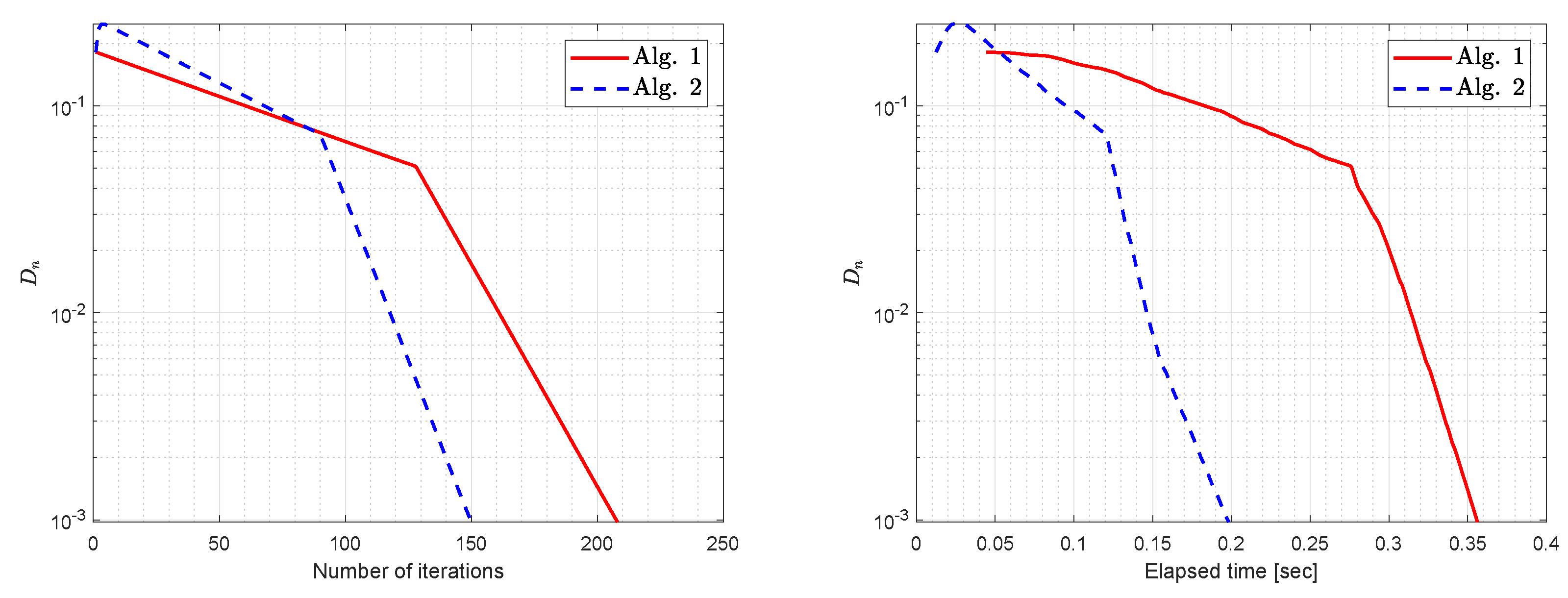
In this section, we consider two numerical examples to explain the efficiency of the proposed algorithms. The MATLAB codes run in MATLAB version 9.5 (R2018b) on Intel(R) Core(TM)i5-6200 CPU PC @ 2.30 GHz 2.40 GHz, RAM 8.00 GB. We use the Quadratic programming to solve the minimization problems.
- (1)
- For Van Hieu results in [23] Algorithm 3.1 (Alg. 1) we use
- (2)
- For our proposed algorithms (Alg. 2) we use and
Example 1.
Let the operators can be define on the convex set as follows:
where is an matrix, is an skew-symmetric matrix and is an diagonal matrix whose diagonal entries are non-negative. All these above mentioned matrices and vectors are randomly generated () between The feasible set is cc set and defined as:
where A is an matrix and d is a non-negative vector. It is clear that is monotone and L-Lipschitz continuous with In this example, we choose Thus, the solution set During Example 1, we use and
Example 2.
Suppose that is a Hs with the norm
and the inner product
Assume that be the unit ball. Let us define an operator by
for all , and i = 1, 2, where
As shown in [14] the is monotone (hence pseudo-monotone) and L-Lipschitz-continuous with Moreover, the solution set of the CSVIPs for the operators on is During example 2, we use and
5. Discussion
We have the following observations concerning the above-mentioned experiments:
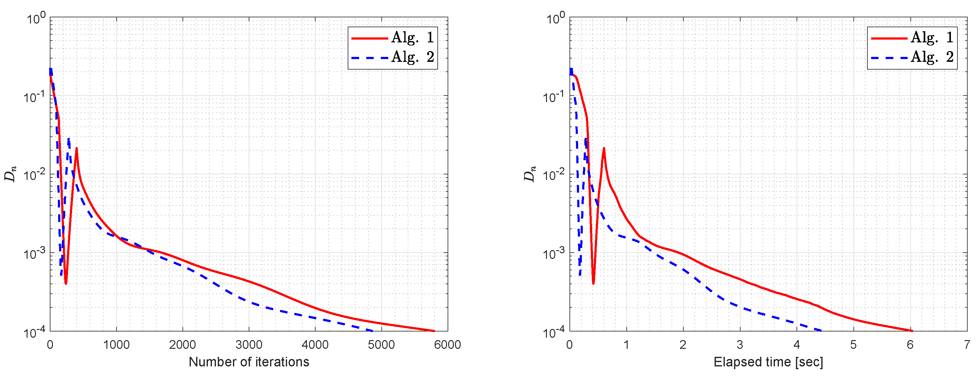
- (i)
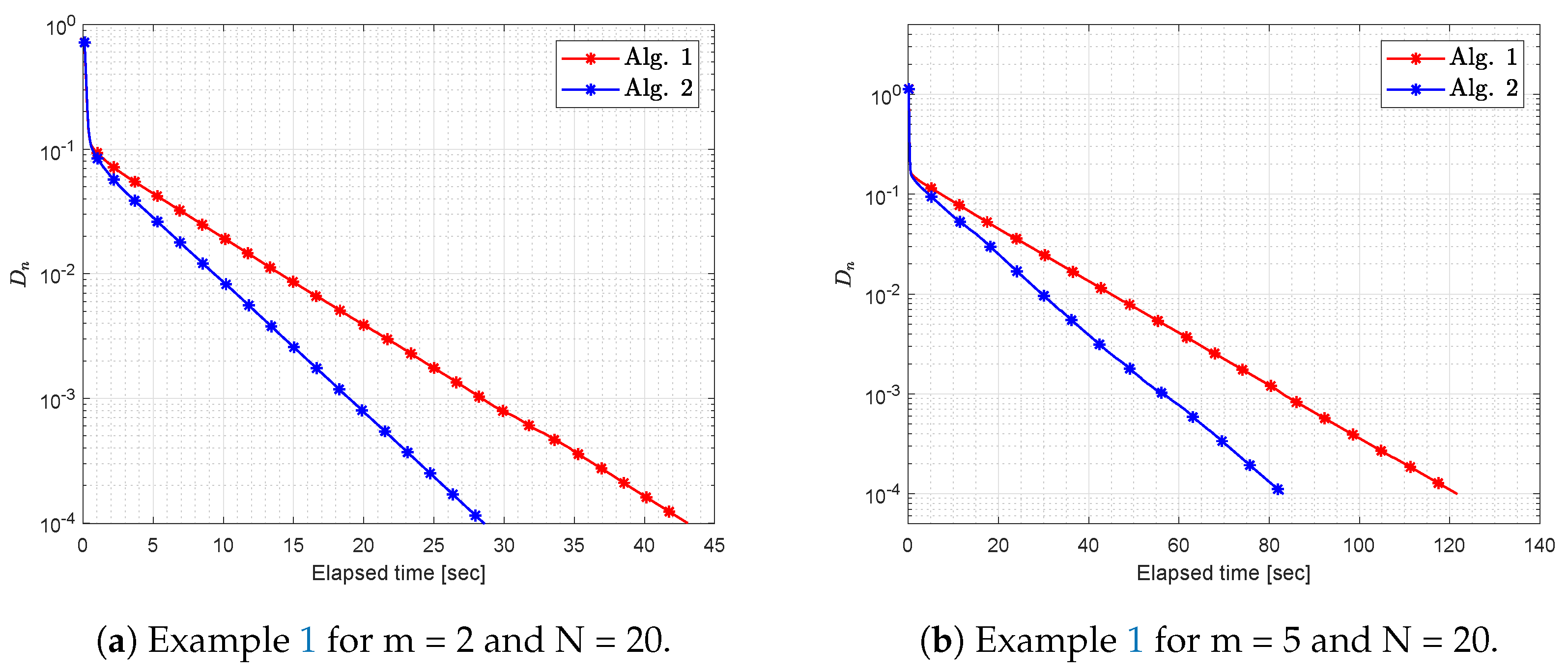
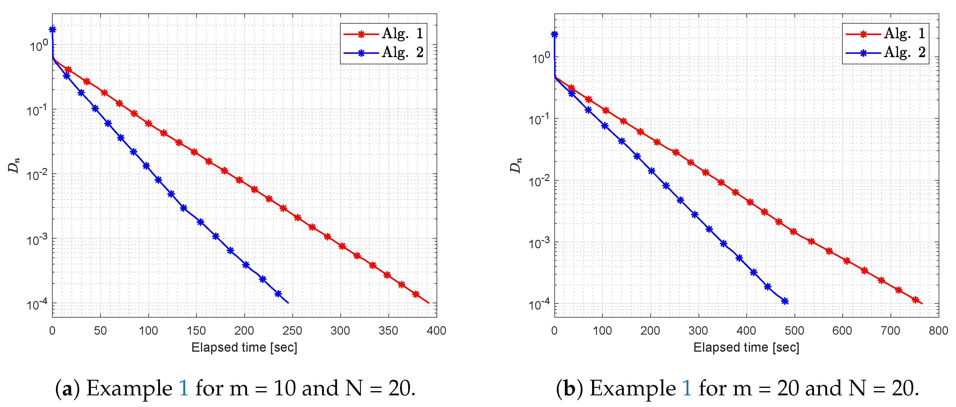
- Figure 1 and Figure 2 and Table 1 demonstrates the behavior of both algorithms as the size of the problem m varies. We can see that the performance of the algorithm depends on the size of the problem. More time and a significant number of iterations are required for large dimensional problems. In this case, we can see that the inertial effect strengthens the efficiency of the algorithm and improves the convergence rate.
- (ii)
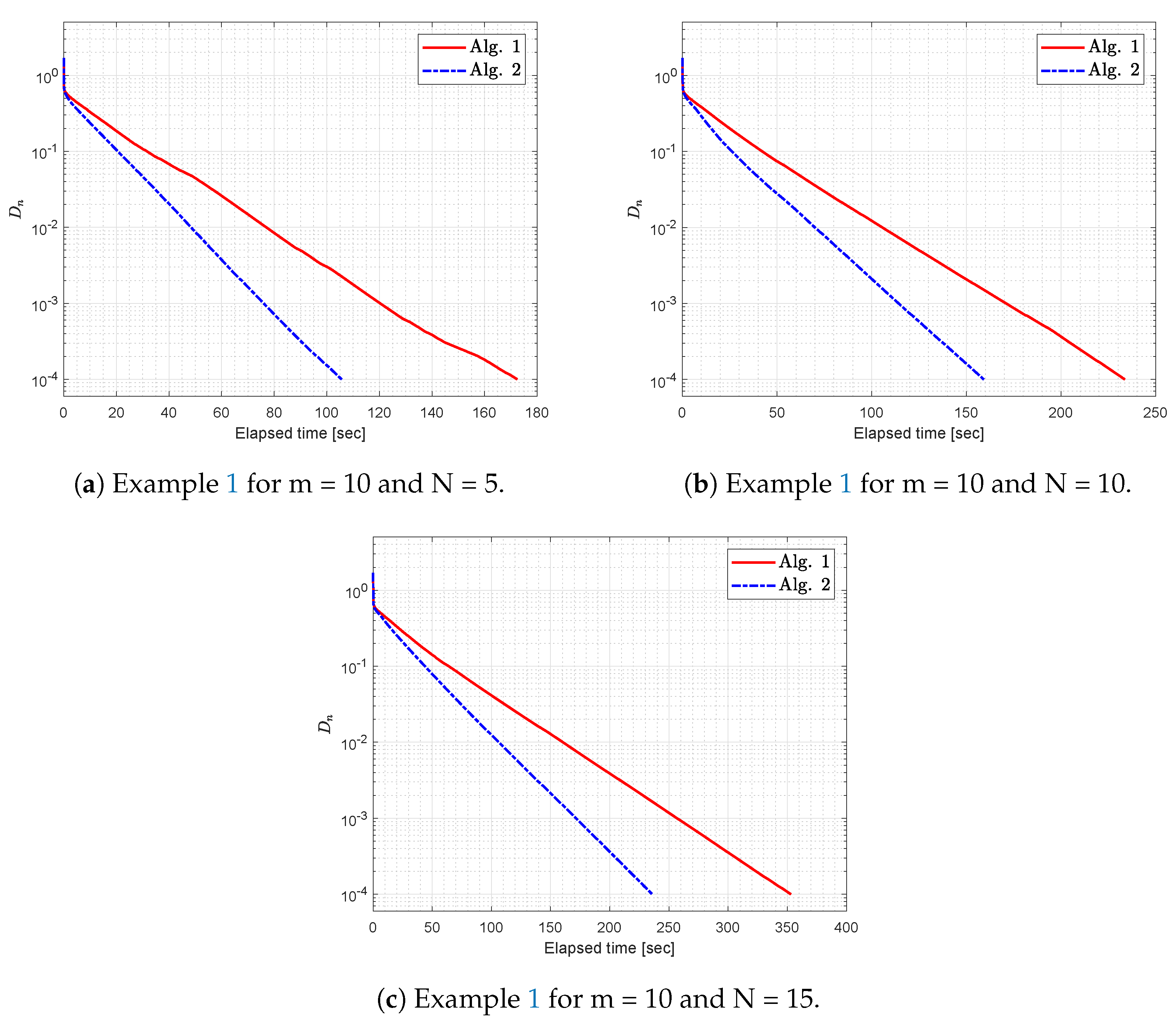
- Figure 3 and Table 2 display the behavior of both algorithms while the number of problems N varies. It could be said that the performance of algorithms also depends on the number of problems involved. In this scenario, we can see that roughly the same number of iterations are required, but the execution time depends entirely on the number of problems N.
- (iii)
- (iv)
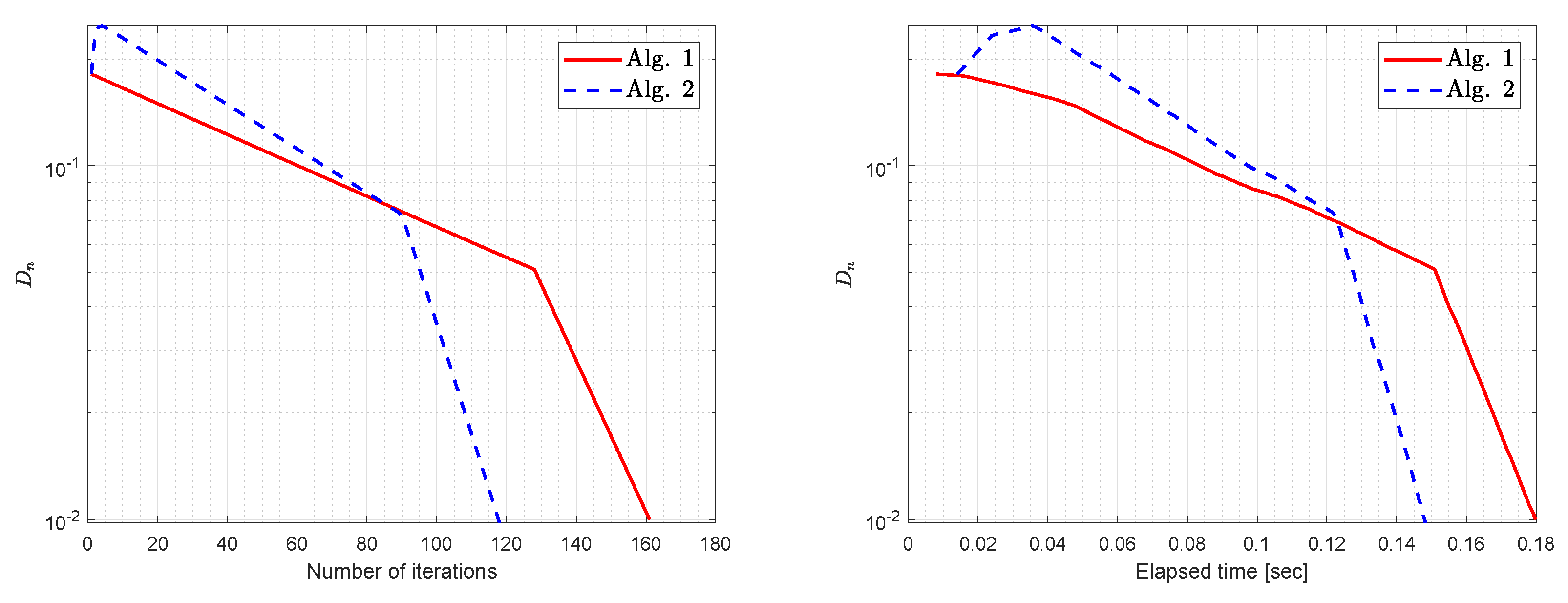
- Based on the progress of the numerical results, we find that our methods are effective and successful in finding solutions for VIP and our algorithms converges faster than the algorithms of Hieu [19].
6. Conclusions
In this manuscript, we propose two strongly convergent parallel and cyclic hybrid inertial CQ-sub-gradient extra-gradient algorithms for finding common the CSVIP. This problem consists of finding a common solution to a system of unrelated variational inequalities corresponding to set-valued mappings in a Hs. The algorithms presented in this article are a hybrid of synthesis the inertial technical, shrinking projection and CQ-terms to parallel and cyclic hybrid inertial sub-gradient extra-gradient algorithms to develop possible practical numerical methods when the number of sub-problems is large. Finally, non-trivial numerical examples are given here to verify the efficiency of the proposed parallel and cyclic algorithms.
Author Contributions
H.A.H. contributed in conceptualization, investigation, methodology, validation and writing the theoretical results; H.u.R. contributed in conceptualization, investigation and writing the numerical results; M.D.l.S. contributed in funding acquisition, methodology, project administration, supervision, validation, visualization, writing and editing. All authors have read and agreed to the published version of the manuscript.
Funding
This work was supported in part by the Basque Government under Grant IT1207-19.
Acknowledgments
The authors are grateful to the Spanish Government and the European Commission for Grant RTI2018-094336-B-I00 (MCIU/AEI/FEDER, UE).
Conflicts of Interest
The authors declare no conflict of interest.
References
- Hartman, P.; Stampacchia, G. On some non-linear elliptic differential-functional equations. Acta Math. 1966, 115, 271–310. [Google Scholar] [CrossRef]
- Aubin, J.P.; Ekeland, I. Applied Nonlinear Analysis; Wiley: New York, NY, USA, 1984. [Google Scholar]
- Baiocchi, C.; Capelo, A. Variational and Quasivariational Inequalities. In Applications to Free Boundary Problems; Wiley: New York, NY, USA, 1984. [Google Scholar]
- Glowinski, R.; Lions, J.L.; Trémolières, R. Numerical Analysis of Variational Inequalities; North-Holland: Amsterdam, The Netherlands, 1981. [Google Scholar]
- Konnov, I.V. Modification of the extragradient method for solving variational inequalities and certain optimization problems. USSR Comput. Math. Math. Phys. 1989, 27, 120–127. [Google Scholar]
- Kinderlehrer, D.; Stampacchia, G. An Introduction to Variational Inequalities and Their Applications; Academic Press: New York, NY, USA, 1980. [Google Scholar]
- Konnov, I.V. Combined Relaxation Methods for Variational Inequalities; Springer: Berlin, Germany, 2001. [Google Scholar]
- Marcotte, P. Applications of Khobotov’s algorithm to variational and network equlibrium problems. Inf. Syst. Oper. Res. 1991, 29, 258–270. [Google Scholar]
- Facchinei, F.; Pang, J.S. Finite-Dimensional Variational Inequalities and Complementarity Problems; Springer Series in Operations Research; Springer: New York, NY, USA, 2003; Volume II. [Google Scholar]
- Korpelevich, G.M. The extragradient method for finding saddle points and other problems. Ekon. Mat. Metod. 1976, 12, 747–756. [Google Scholar]
- Censor, Y.; Gibali, A.; Reich, S. The subgradient extragradient method for solving variational inequalities in Hilbert space. J. Optim. Theory Appl. 2011, 148, 318–335. [Google Scholar] [CrossRef] [PubMed] [Green Version]
- Censor, Y.; Gibali, A.; Reich, S. Strong convergence of subgradient extragradient methods for the variational inequality problem in Hilbert space. Optim. Methods Softw. 2011, 26, 827–845. [Google Scholar] [CrossRef]
- Censor, Y.; Chen, W.; Combettes, P.L.; Davidi, R.; Herman, G.T. On the effectiveness of projection methods for convex feasibility problems with linear inequality constraints. Comput. Optim. Appl. 2011. [Google Scholar] [CrossRef]
- Hieu, D.V.; Anh, P.K.; Muu, L.D. Modified hybrid projection methods for finding common solutions to variational inequality problems. Comput. Optim. Appl. 2017, 66, 75–96. [Google Scholar] [CrossRef]
- Hieu, D.V. Parallel hybrid methods for generalized equilibrium problems and asymptotically strictly pseudocontractive mappings. J. Appl. Math. Comput. 2016. [Google Scholar] [CrossRef] [Green Version]
- Yamada, I. The hybrid steepest descent method for the variational inequality problem over the intersection of fixed point sets of nonexpansive mappings. In Inherently Parallel Algorithms in Feasibility and Optimization and Their Applications; Butnariu, D., Censor, Y., Reich, S., Eds.; Elsevier: Amsterdam, The Netherlands, 2001; pp. 473–504. [Google Scholar]
- Yao, Y.; Liou, Y.C. Weak and strong convergence of Krasnoselski-Mann iteration for hierarchical fixed point problems. Inverse Probl. 2008. [Google Scholar] [CrossRef]
- Bauschke, H.H.; Borwein, J.M. On projection algorithms for solving convex feasibility problems. SIAM Rev. 1996, 38, 367–426. [Google Scholar] [CrossRef] [Green Version]
- Stark, H. Image Recovery Theory and Applications; Academic: Orlando, FL, USA, 1987. [Google Scholar]
- Censor, Y.; Gibali, A.; Reich, S.; Sabach, S. Common solutions to variational inequalities. Set Val. Var. Anal. 2012, 20, 229–247. [Google Scholar] [CrossRef]
- Anh, P.K.; Hieu, D.V. Parallel and sequential hybrid methods for a finite family of asymptotically quasi ϕ-nonexpansive mappings. J. Appl. Math. Comput. 2015, 48, 241–263. [Google Scholar] [CrossRef]
- Anh, P.K.; Hieu, D.V. Parallel hybrid methods for variational inequalities, equilibrium problems and common fixed point problems. Vietnam J. Math. 2015. [Google Scholar] [CrossRef]
- Hieu, D.V. Parallel and cyclic hybrid subgradient extragradient methods for variational inequalities. Afr. Mat. 2016. [Google Scholar] [CrossRef]
- Alber, Y.; Ryazantseva, I. Nonlinear Ill-Posed Problems of Monotone Type; Spinger: Dordrecht, The Netherlands, 2006. [Google Scholar]
- Takahashi, W. Nonlinear Functional Analysis; Yokohama Publishers: Yokohama, Japan, 2000. [Google Scholar]
- Martinez-Yanes, C.; Xu, H.K. Strong convergence of the CQ method for fixed point iteration processes. Nonlinear Anal. 2006, 64, 2400–2411. [Google Scholar] [CrossRef]
- Rockafellar, R.T. On the maximality of sums of nonlinear monotone operators. Trans. Am. Math. Soc. 1970, 149, 75–88. [Google Scholar] [CrossRef]
Figure 1.
Example 1: Numerical comparison for the values of m = 2, 5 and N = 20.

Figure 2.
Example 1: Numerical comparison for the values of m = 10, 20 and N = 20.

Figure 3.
Example 1 for m = 10 and different values of N = 5, 10, 15.

Figure 4.
Example 2: Numerical comparison by letting TOL = .

Figure 5.
Example 2: Numerical comparison by letting TOL = .

Figure 6.
Example 2: Numerical comparison by letting TOL = .


| N | m | Algorithm 1 | Algorithm 2 | ||
|---|---|---|---|---|---|
| Number of Iter. | CPU (s) | Number of Iter. | CPU (s) | ||
| 20 | 2 | 269 | 43.01771 | 185 | 28.6043 |
| 20 | 5 | 788 | 121.0213 | 529 | 83.1379 |
| 20 | 10 | 2493 | 391.9032 | 1066 | 245.6833 |
| 20 | 20 | 7780 | 765.5070 | 3038 | 485.9237 |
Table 2.
Numerical results for Figure 3.
Table 2.
Numerical results for Figure 3.
| N | m | Algorithm 1 | Algorithm 2 | ||
|---|---|---|---|---|---|
| Number of Iter. | CPU (s) | Number of Iter. | CPU (s) | ||
| 5 | 10 | 3101 | 172.4298 | 2267 | 105.7254 |
| 10 | 10 | 3009 | 233.6499 | 2340 | 159.1928 |
| 15 | 10 | 3254 | 353.0176 | 2109 | 235.8372 |
© 2020 by the authors. Licensee MDPI, Basel, Switzerland. This article is an open access article distributed under the terms and conditions of the Creative Commons Attribution (CC BY) license (http://creativecommons.org/licenses/by/4.0/).
Share and Cite
MDPI and ACS Style
Hammad, H.A.; ur Rehman, H.; De la Sen, M. Advanced Algorithms and Common Solutions to Variational Inequalities. Symmetry 2020, 12, 1198. https://0-doi-org.brum.beds.ac.uk/10.3390/sym12071198
AMA Style
Hammad HA, ur Rehman H, De la Sen M. Advanced Algorithms and Common Solutions to Variational Inequalities. Symmetry. 2020; 12(7):1198. https://0-doi-org.brum.beds.ac.uk/10.3390/sym12071198
Chicago/Turabian StyleHammad, Hasanen A., Habib ur Rehman, and Manuel De la Sen. 2020. "Advanced Algorithms and Common Solutions to Variational Inequalities" Symmetry 12, no. 7: 1198. https://0-doi-org.brum.beds.ac.uk/10.3390/sym12071198
Note that from the first issue of 2016, this journal uses article numbers instead of page numbers. See further details here.