Rational Transfer Function Model for a Double-Pipe Parallel-Flow Heat Exchanger


Institute of Control Engineering, Opole University of Technology, ul. Prószkowska 76, 45-758 Opole, Poland
Symmetry 2020, 12(8), 1212; https://0-doi-org.brum.beds.ac.uk/10.3390/sym12081212
Submission received: 1 July 2020
/
Revised: 21 July 2020
/
Accepted: 22 July 2020
/
Published: 23 July 2020
(This article belongs to the Special Issue Symmetry in Dynamic Systems)
Abstract
:Transfer functions of typical heat exchangers, resulting from their partial differential equations, usually contain irrational functions which quite accurately describe the spatio-temporal nature of the processes occurring therein. However, such an accurate but complex mathematical representation is often not convenient from the practical point of view, and some approximation of the original model would be more useful. This paper discusses approximate rational transfer functions for a typical thick-walled double-pipe heat exchanger working in the parallel-flow configuration. Using the method of lines with the backward difference scheme, the original symmetric hyperbolic partial differential equations describing the heat transfer phenomena are transformed into a set of ordinary differential equations and expressed in the form of N subsystems representing spatial sections of the exchanger. Each section is described by a rational transfer function matrix and their cascade interconnection results in the overall approximation model expressed by a matrix of rational transfer functions of high order. Based on the rational transfer function representation, the frequency and steady-state responses of the approximate model are evaluated and compared with those resulting from its original irrational transfer function model. The presented results show better approximation quality for the “crossover” input–output channels where the in-domain heat conduction effects prevail as compared to the “straightforward” channels, where the transport delay associated with the heat convection dominates.
1. Introduction
Contemporary mathematical models of heat exchange processes describe not only their steady-state behavior but also their dynamic properties, which are relevant, e.g., to design effective control algorithms. The first, relatively simple attempt is the process representation as the lumped parameter system (LPS), usually in the form of ordinary differential equations (ODEs) which can describe dynamically changing phenomena, such as temperature or flow variations in time. However, in the case where the spatial effects cannot be neglected or averaged without significant loss of model quality, it needs to be considered to be the distributed parameter system (DPS). Such models are mostly described by partial differential equations (PDEs), and this approach is not uncommon for the phenomena taking place, e.g., inside different types of heat exchangers. Therefore, a lot of attention has been devoted so far in the literature to the PDE-based modeling of these thermal devices, which are often described by hyperbolic equations resulting from the balance laws of continuum physics. The development of the PDE-based phenomenological modeling methods progressed in two parallel directions, with the use of either analytical [1,2,3,4,5,6,7,8] or numerical [9,10,11,12,13,14,15] approaches. The other approach consists of using data-based techniques, also known as black-box modeling or process identification [16,17,18], or even in using artificial neural networks [19,20,21]. The so-called gray-box modeling approach, which combines qualitative prior knowledge with quantitative data, can also be used here [22,23,24].
Although strictly based on the process phenomenology and thus very precise, PDE models have some practical drawbacks which makes them not very convenient, e.g., for the control system design. This is mainly due to the fact that they do not express directly the relationships between the output (controlled) and the input (manipulated) variables of the modeled system, which is of great importance from the control point of view. However, such features are typical of the transfer function representation, which is commonly used, e.g., within signal processing and control systems engineering. The main advantage of this method is that the knowledge of the transfer function of the system allows determining its steady-state, as well as frequency- and time-domain responses, focusing on the relationship between its input and output signals. Consequently, it constitutes a convenient starting point for computer-based implementation of different control algorithms.
Therefore, many works in the literature have been devoted so far to the transfer function-oriented modeling of heat exchange phenomena. These models are often expressed by the extremely simplified transfer functions, such as first or second order with time delay, which may, however, be useful for some applications such as control design [25,26,27]. On the other hand, there are some papers where the more accurate, irrational transfer function models are considered which are derived from the PDE representation of the heat exchange processes [28,29,30,31,32]. The author’s works [33,34] can also be included into this category. However, such irrational transfer functions, although accurately describe the spatio-temporal nature of the heat exchange process, bring some difficulties to the practical implementation. As stated in [9], their complex transcendental form makes them inconvenient to use in standard control system design and simulation methods.
In the current paper we consider transfer function representation for a typical double-pipe heat exchanger, which can be seen as an intermediate between both of the above-mentioned approaches. We start with the infinite-dimensional process representation in the form of symmetric hyperbolic PDEs, which are typical of engineering processes such as heat exchangers, gas absorbers, tubular reactors and irrigation canals [35]. Next, we apply the so-called method of lines (MOL) which transforms the model to the high- but finite-dimensional representation in the form of ordinary differential equations (ODEs). Consequently, we obtain high-order rational transfer function model of the exchanger which is much more accurate than the simple first-order-with-delay transfer functions mentioned above. Such a model can approximate the dominant dynamic behavior of the original system while being accurate enough for control and analysis needs. As far as it is known to the author, only a few papers have analyzed rational transfer function models for heat exchangers in such way, i.e., starting from their PDE representation. One of these few is the work by [36], wherein the rational transfer function model is obtained from the irrational one by rationalization of its irrational terms, and another is the paper [37] where coupled linearized PDEs are reduced into low-order nominal process models using the so-called orthogonal collocation method.
The remainder of the paper is ordered as follows. Section 2 recalls the results of our paper [34] concerning mathematical models for a thick-walled double-pipe heat exchanger in the form of PDEs and resulting irrational transfer functions. Section 3 presents the transformation of the PDE into the ODE representation using method of lines, and derivation of approximate rational transfer functions. Section 4 compares the frequency-domain and steady-state responses evaluated based on the original transfer function representation and the approximate transfer function models of different orders. Finally, Section 5 gives a conclusion and future work prospects.
2. Distributed Parameter Model of the Heat Exchanger
One of the most simple and applicable heat exchangers are the double-pipe ones. They are widely used in chemical, food, oil and gas industries [38]. Despite their simplicity and relatively low efficiency, double-pipe heat exchangers are very important also due to their educational value in teaching the basics of heat exchanger design and control (see Figure 1). Besides, they form the structural basis for many more complex constructions, such as, e.g., shell-and-tube heat exchangers or steam generators [34]. This type of heat exchanger consists of two concentric tubes through which flow heat exchanging fluids, from the inlet of each tube towards its outlet (Figure 2). Usually, hot process fluid flows through the inner pipe and transfers its heat to the cold one flowing in the outer pipe. To distinguish them from each other, the external tube will be referred as shell and the internal—as wall or simply as tube. Depending on the flow directions, we can distinguish two exchanger operation modes. The parallel-flow (or co-current) configuration is when the flow of the two streams is in the same direction, and the counter-flow (or counter-current) one is when the flow of the streams run in opposite directions. In this paper, we focus on the first case.
2.1. Governing PDEs
For the purpose of developing the mathematical model of the heat exchanger of Figure 2, we use the energy balance equations with the following simplifying assumptions [4,28,34,39,40]:
- exchanger is perfectly insulated from the environment;
- there are no internal thermal energy sources inside;
- the flows are sufficiently turbulent to cause effective heat transfer;
- only forced heat convection is considered (i.e., longitudinal heat conduction within the fluids and wall is neglected);
- pressure drops of fluids along the shell and the tube are negligible;
- the densities and heat capacities of the shell, tube and fluids are time and space invariant;
- the convective heat transfer coefficients are constant and uniform over each surface.
Taking into account the above simplifications, the dynamical properties of the double-pipe heat exchanger depicted in Figure 2 are governed by the following hyperbolic PDE system:
where represents time, is the space variable and , , , are constant parameters depending on the shell and tube diameters, physical parameters of the fluids and the material of the exchanger:
where d is the diameter, is the density, c is the specific heat and h is the heat transfer coefficient (subscripts as for the temperatures in Figure 2). Since both matrices of coefficients on the left side of Equations (1)–(3) are diagonal, and thus symmetric, the considered system can be classified as symmetric hyperbolic system of balance laws [35].
To provide a unique solution of the PDEs (1)–(3), the appropriate initial and boundary conditions need to be specified. The initial conditions can be assumed by the following expressions:
where are functions describing the initial temperature profiles along the exchanger.
Furthermore, the boundary conditions will depend here on one of the flow configurations shown in Figure 2. In this paper, we consider parallel flow with and , for which the boundary conditions can be written in the following form:
where and represent the inlet temperatures of the tube- and the shell-side fluids, respectively, i.e., their temperatures measured at . Therefore, from the control theory point of view, these inlet temperatures can be seen as the boundary input signals to the heat exchanger system. Their variations in time affect the temperature distribution of both fluids along the exchanger, and, most importantly, their outflow temperatures at ,
which in turn, can be seen as the boundary output signals.
The input signals given by Equation (6) can be considered either as controls or disturbances. More precisely, the inlet temperature of the heating tube-side fluid can be taken as the control signal, whereas the variations in the inlet temperature of the heated shell-side fluid can be seen as disturbances. The typical control task is here to stabilize the outlet temperature of the heated shell-side fluid given by (7) on the desired setpoint, in the presence of disturbances caused by variations in given by (6).
2.2. Distributed Transfer Function Model
As follows from the comments in the introductory Section 1 and at the end of Section 2.1, it would be desirable to apply here some kind of mathematical representation of the input–output relationship between the boundary temperatures of the exchanger. Such a representation, expressed in the Laplace transform domain, is commonly used in the fields of signal processing and control theory and known as the transfer function of a dynamical system. Below, we recall results on the transfer function representation of the considered double-pipe heat exchanger which were presented in our work [34]. Since we are dealing with the distributed parameter system, we consider here the distributed transfer functions , where the value of the transfer function depends not only of the complex variable s, but also on the spatial position l at which this transfer function is evaluated.
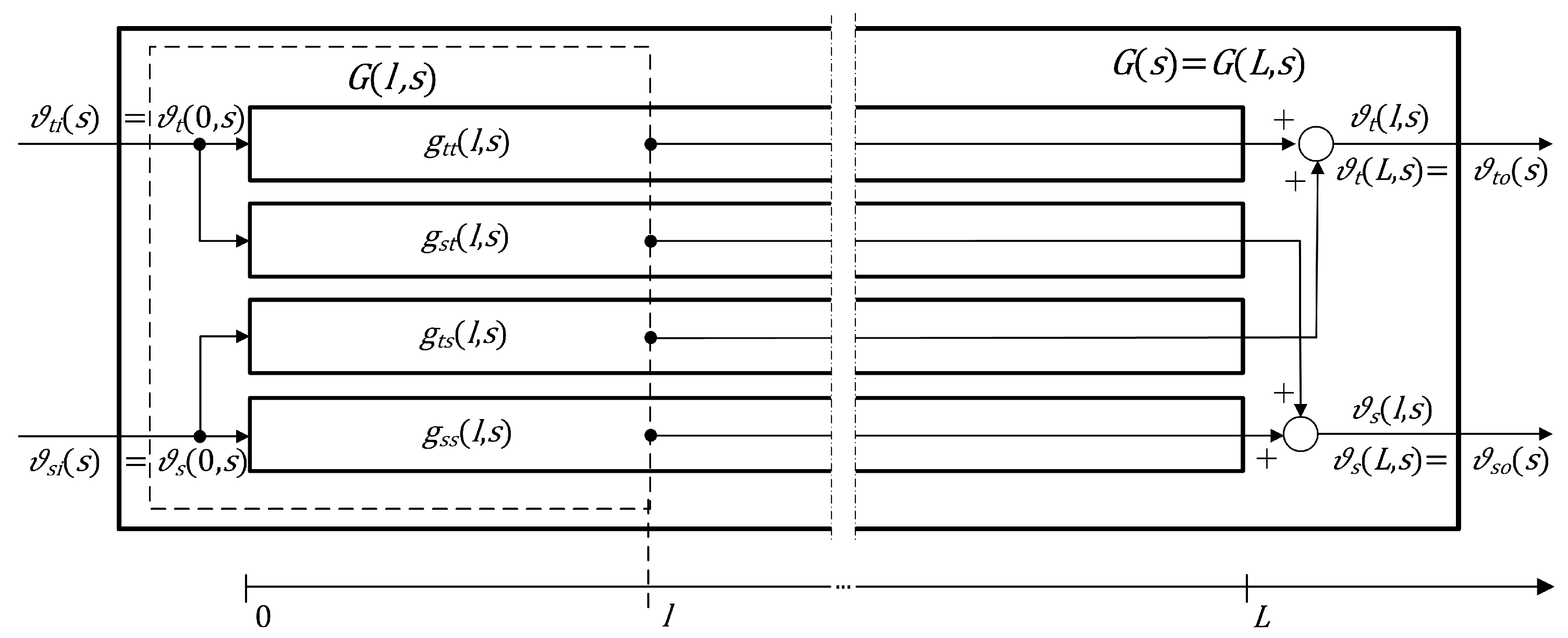
Distributed transfer functions of the heat exchanger working in the parallel-flow configuration with the boundary inputs given by Equation (6) can be written in the following matrix form:
where
assuming zero initial conditions in Equation (5). The symbol in (9) denotes the Laplace transform of the function in the time-domain variable t. We assume here that in the expression the parameter s alone indicates the Laplace transform. The block diagram of the distributed transfer function model for the considered parallel-flow double-pipe heat exchanger is presented in Figure 3. As shown in the diagram, the temperature distribution of both fluids along the axis of the exchanger can be expressed in the Laplace transform domain, assuming zero initial conditions, by the following equations:
where and are the Laplace-transformed tube- and shell-side fluid inlet temperatures given by Equation (6).
As shown in Section 3.1 of [34], the individual transfer functions in (9) take the following form:
where
and
with
The irrational form of the transfer functions given by Equations (12)–(18) is manifested by the exponential functions appearing therein, resulting from the heat convection taking place inside the pipes, as well as by the square root function in Equation (18) which is typical, among others, of heat conduction phenomena. Therefore, these transfer functions can also be classified as the fractional ones which have received increasing attention in the literature (see, e.g., [41]).
Assuming in Equations (8)–(15), we obtain the boundary transfer functions of the heat exchanger, i.e., the transfer functions representing the relationships between the boundary inputs , in Equation (6) and the boundary outputs , in Equation (7)—see also Figure 3.
Zero heat conduction. For this special case we have in Equation (4) and, consequently, in Equations (1)–(3). As a result, we get in Equations (16)–(18), and, consequently,
which results in the transfer function matrix (8) of the following simple form:
being the time delays of the tube- and shell-side fluids, respectively.
Therefore, the resulting dynamical system can be now seen as two separate pure time-delay subsystems with the time delays and given by (20), representing two fluids “traveling” along the exchanger with unchanged inlet temperature profiles, and .
2.3. Frequency-Domain Responses
Frequency-domain analysis of a dynamical system shows how the energy of the input signal(s) is distributed inside the system over a range of frequencies. It is closely related to the transfer function representation of the system. To obtain the frequency responses of the considered heat exchanger, the operator variable s in the expressions for the transfer functions presented in Section 2.2 needs to be replaced with the expression , where is the angular frequency. This operation transforms the system representation from the Laplace transform domain to the Fourier transform domain, which, in turn, can be seen as the frequency-domain description of the system.
In the considered case of DPS, the graphical representation of its frequency responses can take the form of three-dimensional graphs, showing their dependence on both the angular frequency and the space variable l. Another possibility is their representation in the form of classical two-dimensional plots, determined for the fixed value of the space variable, e.g., for the exchanger outflow point (see Figure 2). These responses can be represented in several ways, of which two are most commonly used in control theory: Nyquist and Bode plots. The Bode plot is a combination of a magnitude plot, expressing the magnitude of the frequency response, and a phase plot, expressing the phase shift. The expressions for the logarithmic magnitude and phase take here the following form [39]:
respectively, where the expressions for the modulus and argument of the frequency response are as follows:
In the case of the Nyquist plot, the real part of the transfer function is plotted on the X axis (assuming a fixed value of l, e.g., ), whereas the imaginary part is plotted on the Y axis.
Some specific examples of the frequency response plots for the considered parallel-flow heat exchanger are shown later in Section 4. The “exact” frequency responses, i.e., the responses resulting from the irrational transfer functions introduced in Section 2.2, are there compared to the frequency responses obtained from the approximate rational transfer functions derived later in Section 3.
2.4. Steady-State Temperature Distribution
In the case of LPSs, where the spatial effects are neglected or averaged, their steady-state solutions provide information about the static input–output mappings of the system. For the DPSs which are usually mathematically described by PDEs, their steady-state solutions also contain information about the fixed distribution of the physical quantities inside their spatial domains. Therefore, for the double-pipe heat exchanger considered here, the steady-state solution provides not only information about the constant outlet temperatures and of both fluids in the thermodynamic equilibrium conditions, but it also describes constant temperature profiles , and along the axis of the exchanger, which may be of great importance, e.g., from a technological point of view.
As shown in our paper [34], the constant steady-state solution for the considered heat exchanger can be obtained by assuming all time derivatives in Equations (1)–(3) equal to zero, and solving the resulting boundary value problem with the boundary conditions (6) representing constant inlet temperatures and of both fluids. An equivalent way to obtain this solution is based on the insight that the steady-state responses can be seen as the specific case of the frequency-domain responses evaluated for . Therefore, they can be obtained by assuming in the transfer functions presented in Section 2.2. Following this idea, the steady-state temperature profiles and of the tube- and shell-side fluids, respectively, can be determined, based on Equations (10) and (11) with and constant inlet temperatures and , from the following formulas:
where
are the steady-state versions of the transfer functions (12)–(15), with , , , and given by (16)–(18).
Having determined the steady-state distribution of both fluids from Equations (23)–(25), it is possible to calculate also the steady-state temperature profile for the wall from the steady-state version of Equation (2) as
An example of the steady-state temperature distribution for the considered parallel-flow double-pipe heat exchanger is shown later in Section 4, together with its approximation resulting from the rational transfer function model.
3. Approximate Model of the Heat Exchanger
This section deals with the finite-dimensional approximation of the double-pipe heat exchanger model discussed in Section 2. Using the so-called method of lines—which enables reduction of a PDE to a set of ODEs—the approximations of the irrational transfer functions presented in Section 2.2 are derived in the form of rational transfer functions. Next, the frequency-domain and the steady-state analyses of the approximation model are performed.
3.1. Mol Approximation
The method of lines (MOL) involves replacing the spatial derivatives in a PDE by their finite difference approximations. Consequently, only the time variable remains in the resulting expressions which then become ODEs [42,43]. To obtain the MOL-based approximation model of the considered heat exchanger, we here use the finite difference method. For the assumed parallel-flow configuration with both positive fluid velocities, and , we use the backward difference approximation for both Equations (1) and (3). This implies replacing the spatial derivatives in these equations with their following algebraic approximations:
where
represent the tube- and shell-side temperatures, respectively, evaluated at the spatial discretization points for , assuming , , and
is the spatial grid size. In general, can have different values for different n, which means that the individual points of the grid can be unevenly distributed over the spatial range.
As a result, the approximation of the PDEs (1)–(3) takes the form of a system consisting of 3N ODEs, with the following three equations representing single nth spatial section of the exchanger:
for , with the initial conditions (5) transformed to the following form:
representing initial temperatures evaluated for the nth section at the spatial position .
To specify the details of the mathematical representation of the considered ODE approximation model, we make the following assumptions about its individual sections:
- Each nth section represents a third-order dynamical subsystem with the following vector of the state variables:representing the tube-side, wall and shell-side temperatures, respectively, evaluated at .
- The output vector of each nth section is made of first and third components of its state vector in (34),
- Outputs of the last (Nth) section can be seen as approximations of the boundary outputs (7) of the heat exchanger system,representing the outlet temperatures of the tube- and shell-side fluids, respectively.
- Inputs to the nth section, for , are “connected” to the corresponding outputs of the section ,
- Inputs to the first section () are given directly by the boundary inputs (6) to the heat exchanger system,representing the inlet temperatures of the tube- and shell-side fluids, respectively.
Equations (30)–(32) together with the initial conditions (33) can be seen as a linear state-space representation of the single nth spatial section of the exchanger. These equations can be rewritten in the following compact matrix-vector form, commonly used in control and systems theory:
with
being the state, input and output matrices, respectively. The elements of the initial state vector in Equation (39) are given by the initial temperature values specified by Equation (33). The overall MOL-based approximation model of the heat exchanger can be therefore seen as a cascade interconnection of N spatial sections, each given by ODEs (30)–(32), or, equivalently, by the state-space Equations (39)–(41).
An important issue related to the usefulness of the considered approximation model is the question of its stability. With a view to ensure the stability of the entire approximation model, each section needs to represent a stable dynamical subsystem. To ensure the asymptotic stability of the single section, all eigenvalues of its state matrix in (41) need to be negative. Since all physical parameters in Equations (1)–(4) as well as in Equation (29) are positive, the state matrix is diagonally dominant with negative diagonal entries ensuring stability of the section, and, consequently, of the entire model.
3.2. Rational Transfer Functions
3.2.1. Single Section
Taking into account that the section inputs of the approximation model are given by Equations (37) and (38), and its outputs—by Equation (35), the transfer functions of the single nth section of the approximation model can be written as the following matrix:
where
for zero initial conditions, .
As known from the control theory, the transfer function matrix given by Equations (42) and (43) can be obtained from the following expression describing the transformation from the state-space to the transfer function representation (see, e.g., [39]):
where , and are the state, input and output matrices of the nth section given by (41) and I is the 2 × 2 identity matrix.
It can be shown that using Equation (44) we obtain, after some laborious calculations, the transfer functions in Equations (42) and (43) in the following rational form:
with the numerator (b) and denominator (a) coefficients depending on the system parameters in Equations (1)–(4) and the spatial grid size given by Equation (29).
As follows from (44), the denominator polynomial which is common for all transfer functions in (45) represents the characteristic equation of the section state matrix in (41). This means that the poles of the transfer functions in (45) are equal to the eigenvalues of the matrix (unless zero-pole cancelation occurs). Therefore, the stability analysis performed in Section 3.1 in terms of these eigenvalues remains valid in terms of the poles of .
3.2.2. N-Section Approximation Model
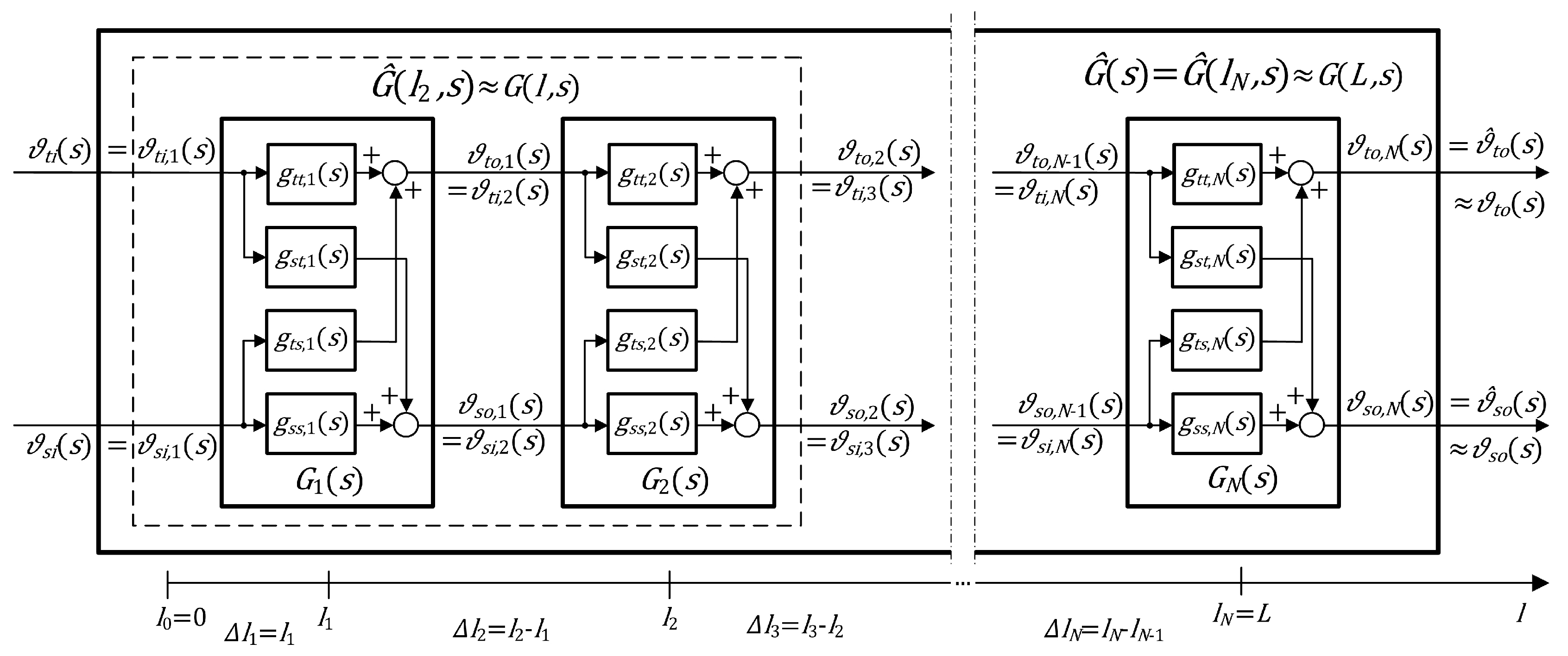
Figure 4 shows the block diagram of the approximation model of the parallel-flow double-pipe heat exchanger represented by the cascade interconnection of N individual sections, each described by the transfer function matrix introduced in Section 3.2.1.
Assuming that there is a need for the evaluation of and at each discretization point , , we introduce the following approximate distributed transfer function matrix :
where
assuming zero initial conditions in (33), with and being the Laplace-transformed tube- and shell-side fluid inlet temperatures in Equation (38).
The transfer function matrix given by Equations (46) and (47) can be therefore seen as a rational approximation of the distributed transfer function matrix discussed in Section 2.2, evaluated at . Since it describes cascade interconnection of n dynamical subsystems, it can be calculated as follows:
where are the transfer function matrices of individual sections discussed in Section 3.2.1.
As shown in the diagram of Figure 4, the approximate temperature distribution of both fluids along the heat exchanger can be expressed in the Laplace-transform domain, assuming zero initial conditions, by the following equations:
for . Assuming in Equation (48) we obtain the approximate boundary transfer function matrix and for this case Equations (49) and (50) describe the relationship between the approximate outlet , and inlet , temperatures of both fluids in the exchanger, expressed in the Laplace transform domain.
3.3. Approximate Frequency-Domain and Steady-State Responses
The frequency-domain responses and the steady-state temperature distribution for the considered approximation model can be evaluated in a similar manner to that outlined in Section 2.3 and Section 2.4, respectively, i.e., based on the approximate transfer function matrix introduced in Section 3.2.2. The approximate logarithmic magnitude and phase are given here by expressions analogous to those for and given by Equations (21) and (22), with the original frequency response replaced with its rational approximation . The spatial variable takes now the values from the finite set which means that for we obtain approximate frequency responses evaluated at , i.e., the approximate boundary frequency responses of the heat exchanger.
Similarly, the approximate steady-state temperature responses and can be calculated based on equations analogous to (23) and (24), with the steady-state transfer functions , , , replaced with their approximations given by
with . For in (51) we obtain from these equations approximate steady-state outflow temperatures and . The steady-state approximate temperature profile of the wall can be determined from an equation similar to (26), with and replaced by their approximations and , respectively.
Visual comparison of the frequency responses and the steady-state temperature distribution obtained from the original, irrational transfer functions of the heat exchanger with the responses resulting from the rational approximation models of different orders (i.e., for different numbers N of spatial sections) can be seen as a simple assessment of the quality of the approximation model. An example of such a comparison is presented in the next section.
4. Results and Discussion
Since the considered double-pipe heat exchanger represents a typical DPS, the “exact” spatio-temporal representation of its dynamics is given by the PDEs introduced in Section 2.1, and alternatively by the irrational transfer functions discussed in Section 2.2. For the simulation purpose we assume the following parameter values in Equations (1)–(4): = 1000 (water), = 7800 (steel), = = 4200 (water), = 500 (steel), = = 6000 , = 0.09 m, = 0.1 m, = 0.15 m, L = 5 m, 1 m/s, = 0.1 m/s.
Turning to the approximation model introduced in Section 3, we assume that the spatial domain is divided, e.g., into uniform sections. Consequently, we obtain the following spatial grid size:
and, for the parameter values assumed above, the following matrices of the state-space model in (41):
with the following negative real eigenvalues of :
implying that the single section represents an exponentially stable dynamical subsystem.
The transformation given by Equation (44) results in the transfer functions matrix of the single section consisting of the following elements:
whose poles are equal to the eigenvalues given by Equation (54).
The cascade interconnection of N uniform sections, each described by the transfer function matrix with the elements given by (55), results in the stable approximation model given by the following approximate distributed transfer function matrix , which can be obtained based on Equation (48) as
Assuming , and, consequently, in Equation (56), we obtain the approximate boundary transfer function matrix of the heat exchanger,
where represents its original irrational boundary transfer function matrix discussed in Section 2.2.
4.1. Frequency Responses
As mentioned in Section 2.3, the frequency responses of the considered heat exchanger can be shown in the form of three-dimensional plots, expressing their dependence on both the angular frequency and the space variable l. Some examples of such 3D Bode plots are presented in our previous work [34]. However, most useful from the practical point of view are the classical two-dimensional Bode and Nyquist plots evaluated at the system outputs, both situated for the considered parallel-flow configuration at . The analysis below compares these plots obtained from the original irrational transfer functions discussed in Section 2.2 and from their rational approximations of different order, introduced in Section 3.2.
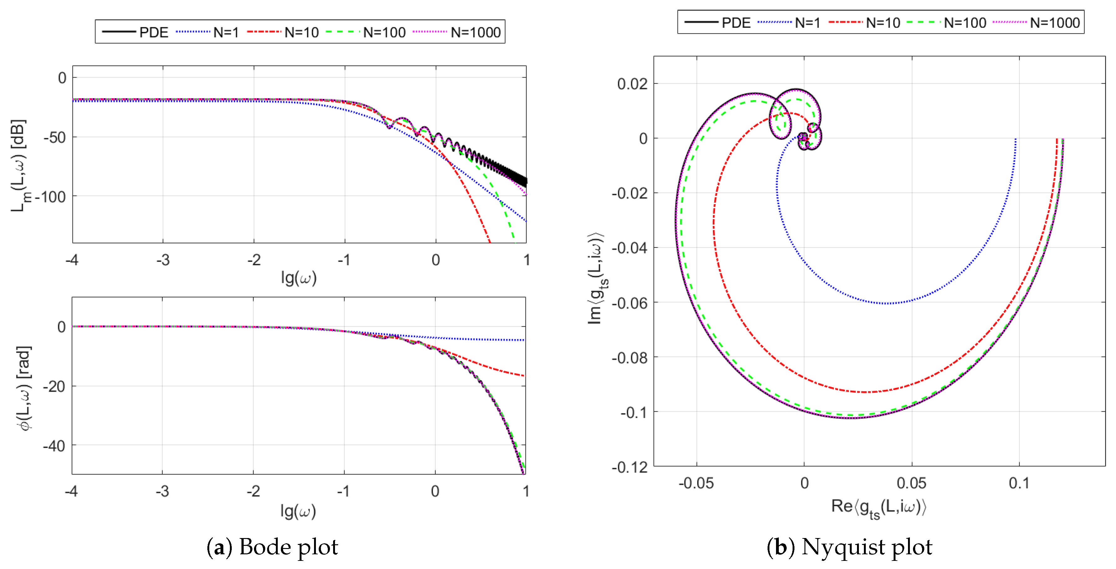
Figure 5 shows the Bode (5a) and Nyquist (5b) plots of the frequency responses evaluated from the boundary transfer function of the considered heat exchanger. These plots contain both the original frequency response obtained from Equations (21) based on the irrational transfer function given by Equation (13), as well as the approximate frequency responses resulting from the approximate rational transfer function discussed in Section 3.2.2.
The oscillations visible in the Bode diagram of Figure 5a, which can be also observed as the “loops” on the Nyquist plot of Figure 5b, are closely associated with the resonance-like phenomena taking place inside the exchanger pipes. They can be observed both in theoretical models as well as in laboratory experiments—see, e.g., [8]. It should be, however, emphasized that the “resonance” occurring in the considered heat exchangers means a periodic fluctuation in the magnitude and the phase of the frequency response and does not mean the resonance used, e.g., in the mechanics [39,44].
Turning to the approximation issue, it can be stated based on the results of Figure 5 that the larger the order of the approximation model, the better the mapping of the original frequency response, together with the above-mentioned “loops” and oscillations. However, in order to correctly map these oscillations, a relatively high order rational model is needed which is able to approximate the high-frequency behavior of the original DPS.
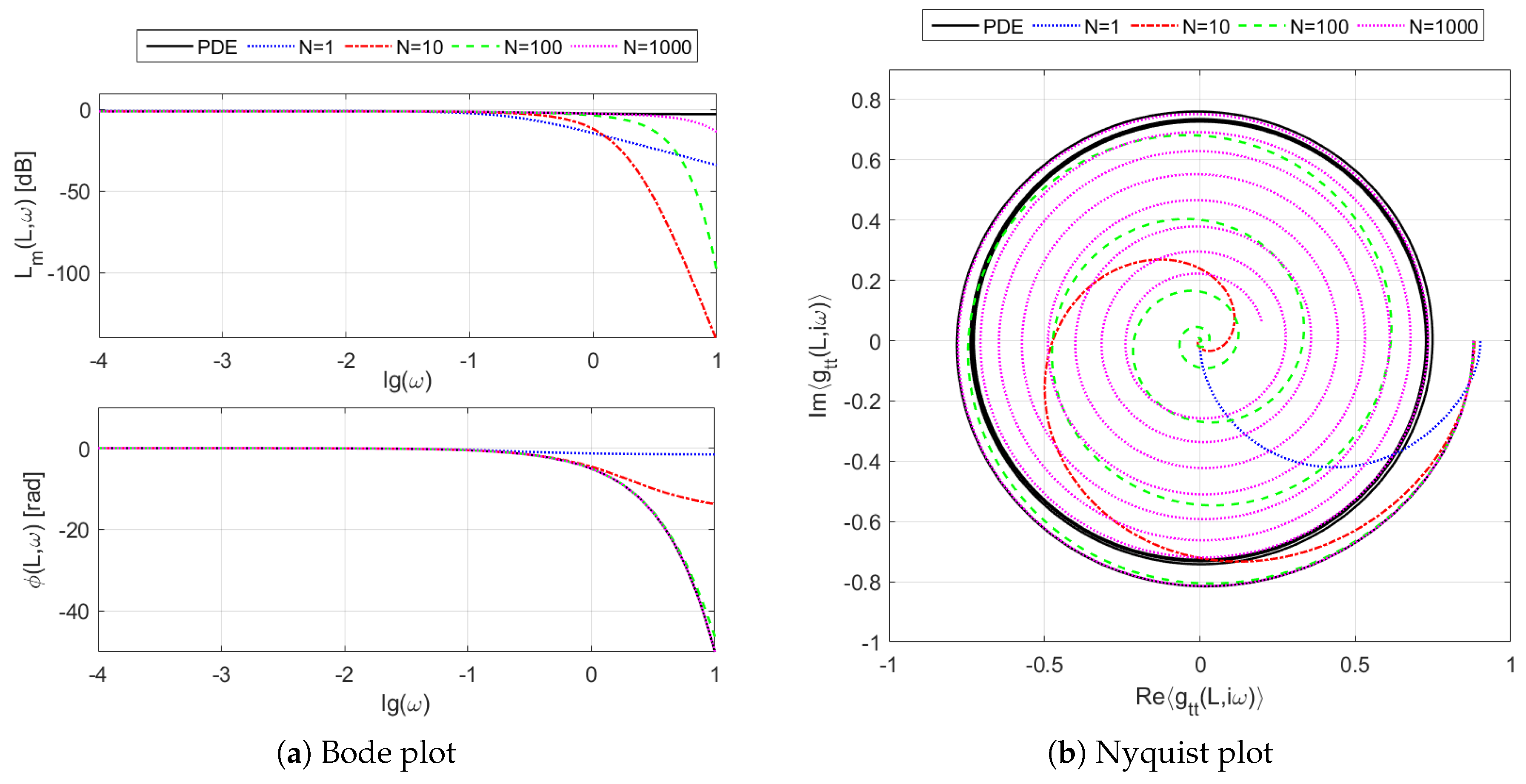
Figure 6 shows the corresponding plots obtained for the transfer function channel . As one can see here, the approximation models of increasing orders try to fit the frequency responses of the original system. However, due to the dominating time-delay nature of this channel, which results in the original frequency response having no limit at infinity, the approximation task is much more difficult here than in the previous case.
The frequency responses of the two remaining transfer function channels, and , which are not shown here for space saving reasons, are similar, due to the symmetry of the system, to the ones obtained for and , respectively, together with their approximation properties.
4.2. Steady-State Temperature Distribution
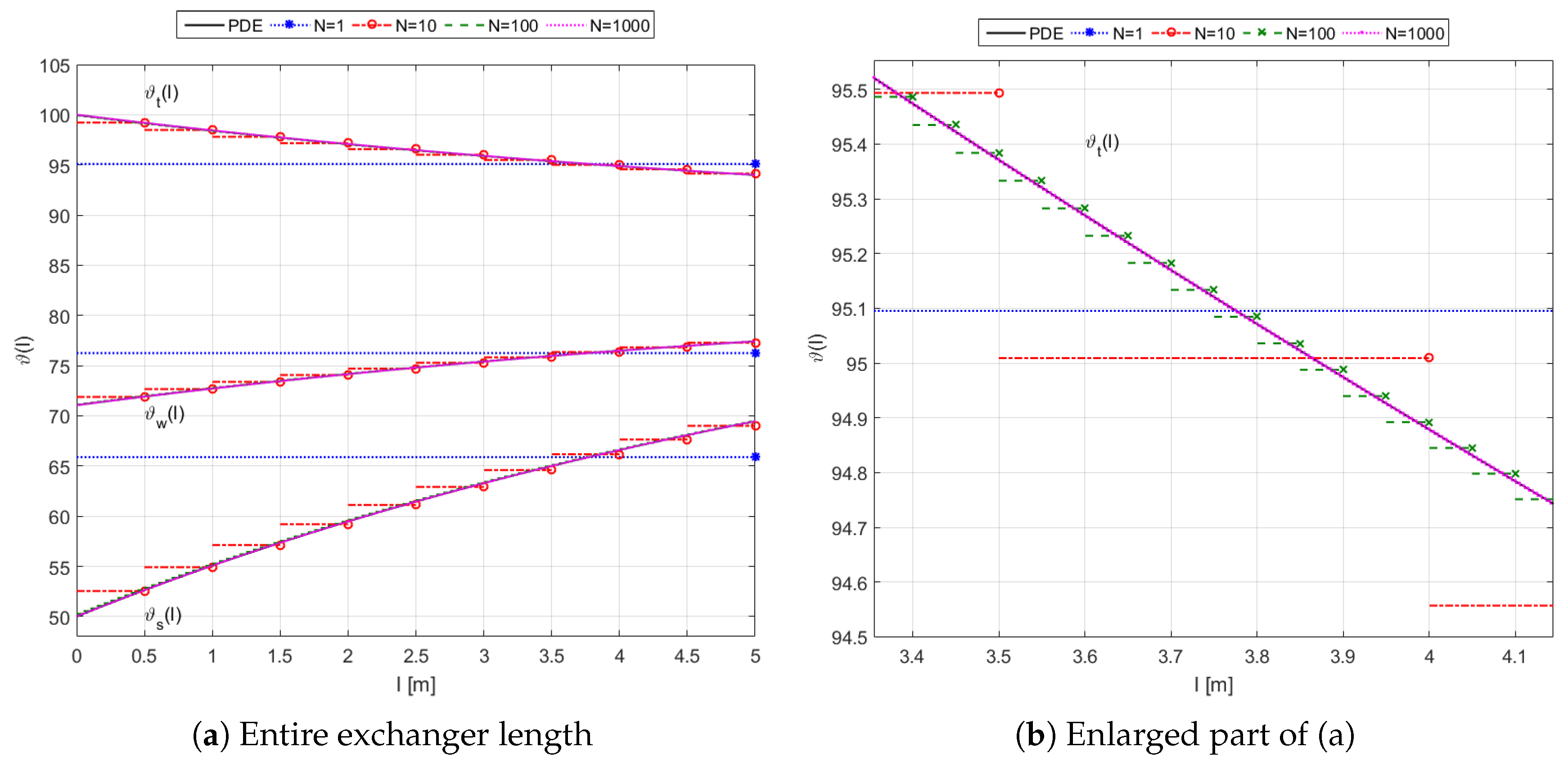
The steady-state temperature profiles of both fluids and the wall were calculated, for the original PDE-based model from Equations (23)–(26), and for the approximation model—from their approximate counterparts discussed in Section 3.3. These profiles obtained for the following constant inlet fluid temperatures: , are presented in Figure 7.
The most important information which can be read from the plot of Figure 7a is the one about the outlet temperatures of both fluids involved in the heat exchange. In the considered example we have: for the heating fluid and for the heated fluid. However, it can be stated that the steady-state temperature distribution of the fluids and the wall obtained for the considered parallel-flow configuration is not so favorable as the one typical of the exchanger working in the counter-flow mode (see [34]). In the latter case, the outlet temperature of the heated fluid can approach the inlet temperature of the heating one, and the more uniform difference between and has an effect of more uniform heat transfer rate. In addition, the uniform temperature difference between the two fluids prevents thermal stresses in the exchanger material.
Turning to the approximation results, it can be read from the plot of Figure 7a that the larger the value of N, the better is the mapping of the original steady-state profiles: , and by their approximations: , and , respectively. To show details of the plot for the high-order models, its enlarged part is shown in Figure 7b.
5. Conclusions and Future Work
In this paper, we presented some results concerning the approximate rational transfer function model for the double-pipe heat exchanger working in the parallel-flow mode. This model can be used, e.g., to perform the controller design for the considered heat exchanger with use of conventional control algorithms, without recourse to complex control algorithms dedicated especially to DPSs. It was shown that within the same dynamical system can exist transfer functions with different approximation properties which strictly depend on the physical phenomena dominating in the given input–output channel. The disadvantage of the presented approach is that the resulting approximation model can be of very high order—even in thousands, as presented in the paper—especially for the channels where transport delay phenomena are dominating. In other words, the resulting rational transfer function model can contain many more parameters as compared to the original irrational transfer function. Therefore, the next step to be performed is to obtain a lower-order model, using the so-called model reduction methods which are able to generate a lower-dimensional approximation of the high-dimensional model while preserving its most important dynamical characteristics. Another option is to use a different approximation approach than the MOL-based strategy presented in the paper, e.g., one of the techniques which have been found effective in the approximation of time-delay systems, such as shift-based approximations or Fourier–Laguerre series.
The quality of the considered approximation models was evaluated in the paper by simple visual comparison of their frequency and steady-state responses with the corresponding responses of the original PDE model. However, in order to perform their quality assessment in a more formal, measurable way, the approximation errors need to be expressed by using, e.g., some of the frequency-domain norms, such as - or -norm. In this paper, we adopted the inlet temperatures of both fluids as the input variables of the transfer function model, assuming constant fluid velocities (flow rates). However, in practical applications, often the flow rate of the heating fluid is taken as the control variable in order to stabilize the outlet temperature of the heated fluid. Also the flow rate of the heated fluid can often vary, e.g., due to the variable heat demand. Therefore, development of transfer function models for this flow-forced case, in both irrational and approximate rational forms, would also be very useful. Future work shall also be carried out on developing similar approximate transfer function model for the double-pipe heat exchanger working in the counter-flow configuration which is usually preferred. Finally, an important task still to be performed is the experimental validation of the considered models using, e.g., the laboratory setup presented in Figure 1, which should include both parallel- and counter-flow configurations.
Funding
This research received no external funding.
Conflicts of Interest
The author declares no conflict of interest.
Symbols and Abbreviations
| Roman Alphabets | |
| A | state matrix |
| a | characteristic polynomial coefficient of A |
| B | input matrix |
| b | transfer function numerator polynomial coefficient |
| C | output matrix |
| c | specific heat [J/(kg·K)] |
| d | pipe diameter [m] |
| i | imaginary unit |
| g | transfer function, frequency response |
| G | transfer function matrix, frequency response matrix |
| h | heat transfer coefficient [W/(m2·K)] |
| k | constant parameter [1/s] |
| L | heat exchanger length [m] |
| logaritmic gain [dB] | |
| l | space variable [m] |
| N | number of sections |
| n | section number |
| p | transfer function subexpression |
| s | complex argument of Laplace transform |
| t | time [s] |
| v | fluid velocity [m/s] |
| Greek Alphabets | |
| first component of | |
| second component of | |
| difference | |
| temperature [°C] | |
| density [kg/m3] | |
| time delay [s] | |
| transfer function subexpression | |
| phase shift [rad] | |
| angular frequency [rad/s] | |
| Subscripts | |
| i | inlet (temperature), inner (diameter) |
| n | nth section |
| o | outlet (temperature), outer (diameter) |
| s | shell-side |
| t | tube-side, time (Laplace transform) |
| w | wall |
| 0 | initial (at t=0) |
| Mathematical Signs | |
| I | identity matrix |
| imaginary part | |
| Laplace transform | |
| set of real numbers | |
| real part | |
| transfer function at | |
| steady state of | |
| approximation of | |
| approximation of | |
| Acronyms | |
| DPS | distributed parameter system |
| LPS | lumped parameter system |
| MOL | method of lines |
| ODE | ordinary differential equation |
| PDE | partial differential equation |
References
- Yin, J.; Jensen, M.K. Analytic model for transient heat exchanger response. Int. J. Heat Mass Transf. 2003, 46, 3255–3264. [Google Scholar] [CrossRef]
- Delnero, C.C.; Dreisigmeyer, D.; Hittle, D.C.; Young, P.M.; Anderson, C.W.; Anderson, M.L. Exact Solution to the Governing PDE of a Hot Water-to-Air Finned Tube Cross-Flow Heat Exchanger. HVAC&R Res. 2004, 10, 21–31. [Google Scholar] [CrossRef]
- Porowski, M. An analytical model of a matrix heat exchanger with longitudinal heat conduction in the matrix in application for the exchanger dynamics research. Heat Mass Transf. 2005, 42, 12–29. [Google Scholar] [CrossRef]
- Ansari, M.R.; Mortazavi, V. Simulation of dynamical response of a countercurrent heat exchanger to inlet temperature or mass flow rate change. Appl. Therm. Eng. 2006, 26, 2401–2408. [Google Scholar] [CrossRef]
- Zavala-Río, A.; Santiesteban-Cos, R. Reliable compartmental models for double-pipe heat exchangers: An analytical study. Appl. Math. Model. 2007, 31, 1739–1752. [Google Scholar] [CrossRef] [Green Version]
- Long, Y.; Wang, S.; Wang, J.; Zhang, T. Mathematical Model of Heat Transfer for a Finned Tube Cross-flow Heat Exchanger with Ice Slurry as Cooling Medium. Procedia Eng. 2016, 146, 513–522. [Google Scholar] [CrossRef] [Green Version]
- Park, S.; Lee, S.; Lee, H.; Pham, K.; Choi, H. Effect of Borehole Material on Analytical Solutions of the Heat Transfer Model of Ground Heat Exchangers Considering Groundwater Flow. Energies 2016, 9, 318. [Google Scholar] [CrossRef] [Green Version]
- Lalot, S.; Desmet, B. The harmonic response of counter-flow heat exchangers—Analytical approach and comparison with experiments. Int. J. Therm. Sci. 2019, 135, 163–172. [Google Scholar] [CrossRef]
- Abu-Hamdeh, N.H. Control of a liquid–liquid heat exchanger. Heat Mass Transf. 2002, 38, 687–693. [Google Scholar] [CrossRef]
- Maidi, A.; Diaf, M.; Corriou, J.P. Boundary geometric control of a counter-current heat exchanger. J. Process Control 2009, 19, 297–313. [Google Scholar] [CrossRef] [Green Version]
- Minkowycz, W.; Sparrow, E.; Abraham, J.; Gorman, J. Advances in Numerical Heat Transfer: Numerical Simulation of Heat Exchangers; CRC Press: Boca Raton, FL, USA, 2017; pp. 1–218. [Google Scholar] [CrossRef]
- Ilori, O.M.; Jaworski, A.J.; Mao, X. Experimental and numerical investigations of thermal characteristics of heat exchangers in oscillatory flow. Appl. Therm. Eng. 2018, 144, 910–925. [Google Scholar] [CrossRef]
- Ke, H.; Lin, Y.; Ke, Z.; Xiao, Q.; Wei, Z.; Chen, K.; Xu, H. Analysis Exploring the Uniformity of Flow Distribution in Multi-Channels for the Application of Printed Circuit Heat Exchangers. Symmetry 2020, 12, 314. [Google Scholar] [CrossRef] [Green Version]
- Nakhchi, M.; Rahmati, M. Entropy generation of turbulent Cu–water nanofluid flows inside thermal systems equipped with transverse-cut twisted turbulators. J. Therm. Anal. Calorim. 2020. [Google Scholar] [CrossRef]
- Nakhchi, M.; Rahmati, M. Turbulent Flows Inside Pipes Equipped With Novel Perforated V-Shaped Rectangular Winglet Turbulators: Numerical Simulations. J. Energy Resour. Technol. 2020, 142. [Google Scholar] [CrossRef]
- Laszczyk, P. Simplified modeling of liquid-liquid heat exchangers for use in control systems. Appl. Therm. Eng. 2017, 119, 140–155. [Google Scholar] [CrossRef]
- Liu, Y.; Korenberg, M.; Billings, S.; Fadzil, M. The nonlinear identification of a heat exchanger. In Proceedings of the 26th IEEE Conference on Decision and Control, Los Angeles, CA, USA, 9–11 December 1987; pp. 1883–1888. [Google Scholar] [CrossRef] [Green Version]
- Sahoo, A.; Radhakrishnan, T.; Rao, C.S. Modeling and control of a real time shell and tube heat exchanger. Resour.-Effic. Technol. 2017, 3, 124–132. [Google Scholar] [CrossRef]
- Bittanti, S.; Piroddi, L. Nonlinear identification and control of a heat exchanger: A neural network approach. J. Frankl. Inst. 1997, 334, 135–153. [Google Scholar] [CrossRef]
- Díaz, G.; Sen, M.; Yang, K.; McClain, R.L. Dynamic prediction and control of heat exchangers using artificial neural networks. Int. J. Heat Mass Transf. 2001, 44, 1671–1679. [Google Scholar] [CrossRef]
- Bartecki, K.; Rojek, R. Instantaneous linearization of neural network model in adaptive control of heat exchange process. In Proceedings of the 11th IEEE International Conference on Methods and Models in Automation and Robotics, Miȩdzyzdroje, Poland, 29 August–1 September 2005; pp. 967–972. [Google Scholar]
- Barszcz, T.; Czop, P. Estimation of feedwater heater parameters based on a grey-box approach. Appl. Math. Comput. Sci. 2011, 21, 703–715. [Google Scholar] [CrossRef]
- Afram, A.; Janabi-Sharifi, F. Gray-box modeling and validation of residential HVAC system for control system design. Appl. Energy 2015, 137, 134–150. [Google Scholar] [CrossRef]
- Miao, Q.; You, S.; Zheng, W.; Zheng, X.; Zhang, H.; Wang, Y. A Grey-Box Dynamic Model of Plate Heat Exchangers Used in an Urban Heating System. Energies 2017, 10, 1398. [Google Scholar] [CrossRef] [Green Version]
- Sharma, C.; Gupta, S.; Kumar, V. Modeling and Simulation of Heat Exchanger Used in Soda Recovery. Lect. Notes Eng. Comput. Sci. 2011, 2, 1406–1409. [Google Scholar]
- Padhee, S. Controller Design for Temperature Control of Heat Exchanger System: Simulation Studies. WSEAS Trans. Syst. Control 2014, 9, 485–491. [Google Scholar]
- Vasičkaninová, A.; Bakošová, M.; Čirka, L.; Kalúz, M.; Oravec, J. Robust controller design for a laboratory heat exchanger. Appl. Therm. Eng. 2018, 128, 1297–1309. [Google Scholar] [CrossRef]
- Stermole, F.J. The Dynamic Response of Flow Forced Heat Exchangers. Ph.D. Thesis, Iowa State University, Ames, IA, USA, 1963. [Google Scholar] [CrossRef]
- Grabowski, P. Abstract Model of a Heat Exchanger and its Application. In Proceedings of the 11th IEEE International Conference on Methods and Models in Automation and Robotics, Miȩdzyzdroje, Poland, 29 August–1 September 2005; pp. 49–54. [Google Scholar]
- Zavala-Río, A.; Astorga-Zaragoza, C.M.; Hernández-González, O. Bounded positive control for double-pipe heat exchangers. Control Eng. Pract. 2009, 17, 136–145. [Google Scholar] [CrossRef]
- Maidi, A.; Diaf, M.; Corriou, J.P. Boundary control of a parallel-flow heat exchanger by input–output linearization. J. Process Control 2010, 20, 1161–1174. [Google Scholar] [CrossRef]
- Gvozdenac, D. Analytical Solution of Dynamic Response of Heat Exchanger. In Heat Exchangers—Basics Design Applications; Mitrovic, J., Ed.; InTech: London, UK, 2012; pp. 53–78. [Google Scholar] [CrossRef]
- Bartecki, K. Comparison of frequency responses of parallel- and counter-flow type of heat exchanger. In Proceedings of the 13th IEEE IFAC International Conference on Methods and Models in Automation and Robotics, Szczecin, Poland, 27–30 August 2007; pp. 411–416. [Google Scholar] [CrossRef]
- Bartecki, K. Transfer function-based analysis of the frequency-domain properties of a double pipe heat exchanger. Heat Mass Transf. 2015, 51, 277–287. [Google Scholar] [CrossRef] [Green Version]
- Xu, C.Z.; Sallet, G. Exponential Stability and Transfer Functions of Processes Governed by Symmetric Hyperbolic Systems. ESAIM Control. Optim. Calc. Var. 2002, 7, 421–442. [Google Scholar] [CrossRef] [Green Version]
- Whalley, R.; Ebrahimi, K. Heat exchanger dynamic analysis. Appl. Math. Model. 2018, 62, 38–50. [Google Scholar] [CrossRef] [Green Version]
- Ding, L.; Johansson, A.; Gustafsson, T. Application of reduced models for robust control and state estimation of a distributed parameter system. J. Process Control 2009, 19, 539–549. [Google Scholar] [CrossRef] [Green Version]
- Omidi, M.; Farhadi, M.; Jafari, M. A comprehensive review on double pipe heat exchangers. Appl. Therm. Eng. 2017, 110, 1075–1090. [Google Scholar] [CrossRef]
- Friedly, J.C. Dynamic Behaviour of Processes; Prentice-Hall: New York, NY, USA, 1972. [Google Scholar]
- Bunce, D.J.; Kandlikar, S.G. Transient response of heat exchangers. In Proceedings of the 2nd ISHMT-ASME Heat and Mass Transfer Conference, Surathkal, India, 28–30 December 1995; pp. 729–736. [Google Scholar]
- Curtain, R.; Morris, K. Transfer functions of distributed parameters systems: A tutorial. Automatica 2009, 45, 1101–1116. [Google Scholar] [CrossRef]
- Koto, T. Method of Lines Approximations of Delay Differential Equations. Comput. Math. Appl. 2004, 48, 45–59. [Google Scholar] [CrossRef] [Green Version]
- Schiesser, W.E.; Griffiths, G.W. A Compendium of Partial Differential Equation Models: Method of Lines Analysis with Matlab; Cambridge University Press: New York, NY, USA, 2009. [Google Scholar]
- Kanoh, H. Distributed parameter heat exchangers—Modeling, dynamics and control. In Distributed Parameter Control Systems: Theory and Application; Tzafestas, S.G., Ed.; Pergamon Press: Oxford, UK, 1982; Chapter 14; pp. 417–449. [Google Scholar]
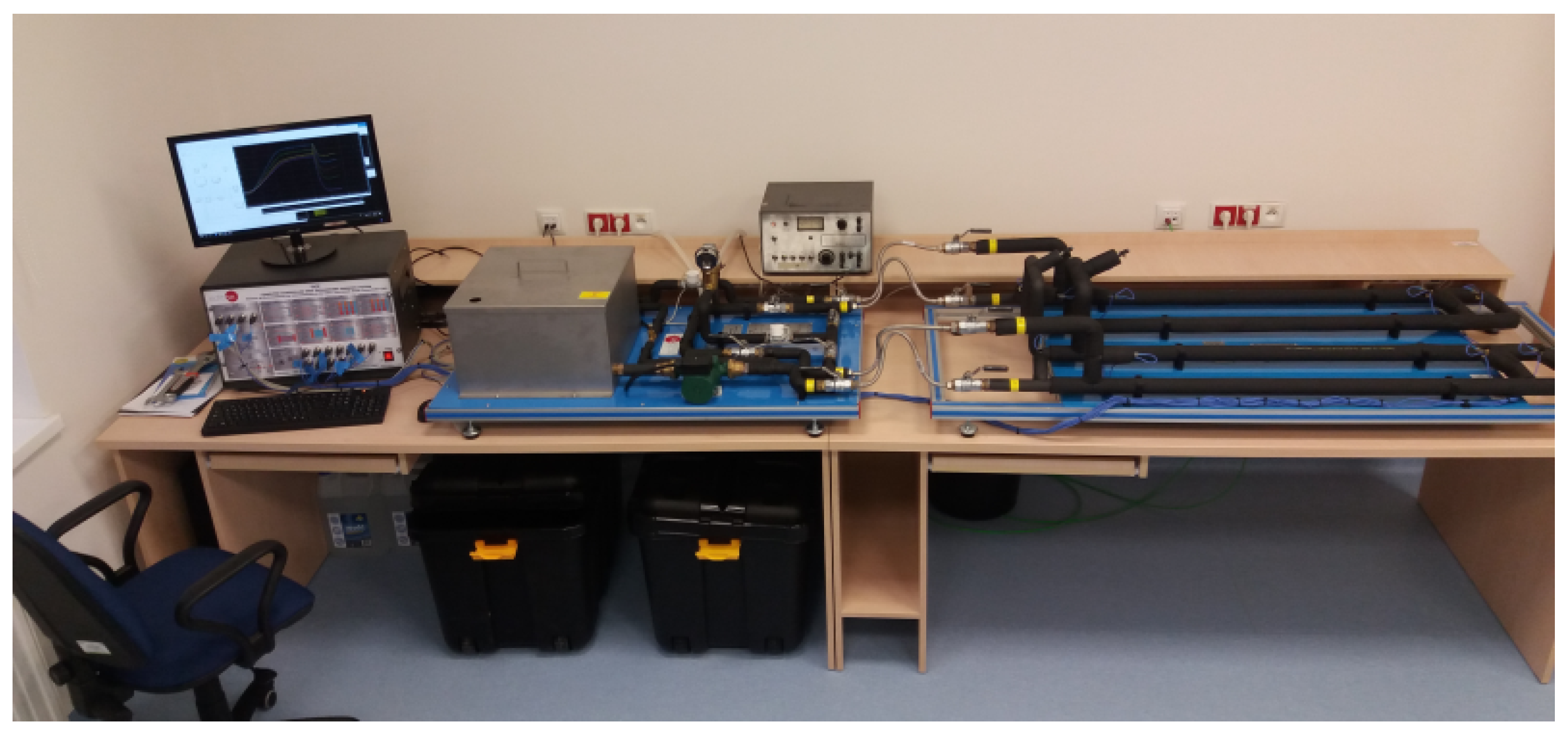
Figure 1.
Double-pipe heat exchanger laboratory setup at the Institute of Control Engineering, Opole University of Technology.
Figure 1.
Double-pipe heat exchanger laboratory setup at the Institute of Control Engineering, Opole University of Technology.

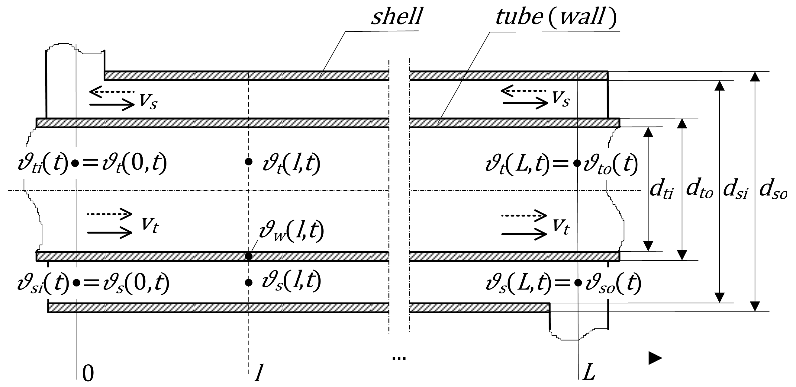
Figure 2.
Schematic of a double-pipe heat exchanger. —shell-side and tube-side fluid velocities; —shell-side and tube-side fluid temperatures; —wall temperature; —shell-side and tube-side fluid inlet temperatures; —shell-side and tube-side fluid outlet temperatures; L—heat exchanger length; —inner and outer diameters of the tube; —inner and outer diameters of the shell. Solid arrows show flow directions for the parallel-flow mode and dotted ones—for the counter-flow mode.

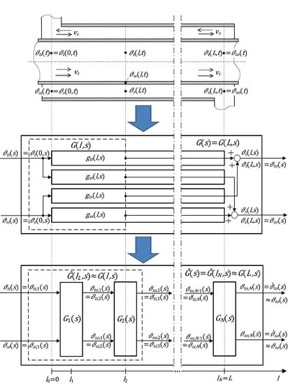
Figure 3.
Block diagram of the distributed transfer function model for the double-pipe parallel-flow heat exchanger.
Figure 3.
Block diagram of the distributed transfer function model for the double-pipe parallel-flow heat exchanger.

Figure 4.
Block diagram of the approximation transfer function model for the double-pipe parallel-flow heat exchanger.
Figure 4.
Block diagram of the approximation transfer function model for the double-pipe parallel-flow heat exchanger.

Figure 5.
Frequency response for the PDE-based model of the double-pipe parallel-flow heat exchanger vs. frequency responses of its approximation models of different orders.
Figure 5.
Frequency response for the PDE-based model of the double-pipe parallel-flow heat exchanger vs. frequency responses of its approximation models of different orders.

Figure 6.
Frequency response for the PDE-based model of the double-pipe parallel-flow heat exchanger vs. frequency responses of its approximation models of different orders.
Figure 6.
Frequency response for the PDE-based model of the double-pipe parallel-flow heat exchanger vs. frequency responses of its approximation models of different orders.

Figure 7.
Steady-state temperature distribution for the PDE-based and approximation models of different orders for the parallel-flow heat exchanger with and .
Figure 7.
Steady-state temperature distribution for the PDE-based and approximation models of different orders for the parallel-flow heat exchanger with and .

© 2020 by the author. Licensee MDPI, Basel, Switzerland. This article is an open access article distributed under the terms and conditions of the Creative Commons Attribution (CC BY) license (http://creativecommons.org/licenses/by/4.0/).
Share and Cite
MDPI and ACS Style
Bartecki, K. Rational Transfer Function Model for a Double-Pipe Parallel-Flow Heat Exchanger. Symmetry 2020, 12, 1212. https://0-doi-org.brum.beds.ac.uk/10.3390/sym12081212
AMA Style
Bartecki K. Rational Transfer Function Model for a Double-Pipe Parallel-Flow Heat Exchanger. Symmetry. 2020; 12(8):1212. https://0-doi-org.brum.beds.ac.uk/10.3390/sym12081212
Chicago/Turabian StyleBartecki, Krzysztof. 2020. "Rational Transfer Function Model for a Double-Pipe Parallel-Flow Heat Exchanger" Symmetry 12, no. 8: 1212. https://0-doi-org.brum.beds.ac.uk/10.3390/sym12081212
Note that from the first issue of 2016, this journal uses article numbers instead of page numbers. See further details here.