Exact and Numerical Solitary Wave Structures to the Variant Boussinesq System


Department of Mathematics, College of Science, Taibah University, P.O. Box 344, Al-Madinah Al-Munawarah 30002, Saudi Arabia
*
Author to whom correspondence should be addressed.
Symmetry 2020, 12(9), 1473; https://0-doi-org.brum.beds.ac.uk/10.3390/sym12091473
Submission received: 19 August 2020
/
Revised: 2 September 2020
/
Accepted: 3 September 2020
/
Published: 8 September 2020
(This article belongs to the Special Issue Ordinary and Partial Differential Equations: Theory and Applications)
Abstract
:Solutions such as symmetric, periodic, and solitary wave solutions play a significant role in the field of partial differential equations (PDEs), and they can be utilized to explain several phenomena in physics and engineering. Therefore, constructing such solutions is significantly essential. This article concentrates on employing the improved -expansion approach and the method of lines on the variant Boussinesq system to establish its exact and numerical solutions. Novel solutions based on the solitary wave structures are obtained. We present a comprehensible comparison between the accomplished exact and numerical results to testify the accuracy of the used numerical technique. Some 3D and 2D diagrams are sketched for some solutions. We also investigate the error and the CPU time of the used numerical method. The used mathematical tools can be comfortably invoked to handle more nonlinear evolution equations.
Keywords:
exact solution; numerical solution; traveling waves; Boussinesq system; L2 error; CPU timeMSC:
35A20; 35A99; 83C15; 65L12; 65N06; 65N40; 65N45; 65N50; 35Q511. Introduction
Most natural phenomena arising in various nonlinear sciences and engineering are modelled by nonlinear evolution equations. More specifically, a dramatic increase in the use of PDEs has been recently seen in some areas such as physics, biology, chemistry, economics, and computer sciences. Equations that describe shallow water waves appear in various fields of physics. The search for finding the exact solutions of such equations has been considerably given more attention in recent years. Although several approaches have been effectively developed, the exact traveling wave solutions for a massive number of NPDEs cannot be obtained. We point out some proposed techniques such as the truncated Painleve expansion process [1], the improved -expansion technique [2], the projective Riccati equation technique [3], the Weierstrass elliptic function method [4], the extended tanh-procedure [5,6], the -expansion process [7,8,9], the sine–cosine approach [10,11], the Adomian decomposition technique [12,13], the Hirota’s bilinear technique [14,15], the inverse scattering transform [16], etc. The availability of some mathematical software such as Matlab, Maple, and Mathematica stimulates mathematicians and scientists to deal with insolvable nonlinear PDEs. Among the available numerical approaches, we state the following: the finite element method, the finite differences, the adaptive moving mesh technique [17], and the Parabolic Monge–Ampere method [18]. For more information about analytical and numerical solutions of NPDEs, one can refer to [19,20,21,22,23,24,25].
This system describes shallow water waves, where indicates the velocity of wave, presents the height of free wave surface, and x and t play the role of the spatial and the temporal derivatives. The constants and are non-zero. The dynamics of shallow water waves are described by the Korteweg-de Vries (KdV) equation. However, the Boussinesq equation perfectly governs shallow water waves and gives much better approximation to such waves [28]. The exact solutions of system (1) have been derived by various scientists. For instance, the authors in [29] presented some traveling wave solutions for system (1) using the -expansion method. Huiqun [26] applied the extended Jacobi elliptic function expansion process to construct some periodic solutions for system (1). The improved ()-expansion technique was used in [27] to extract the exact traveling wave solutions of system (1). Zheng [30] applied the generalized Bernoulli sub-ODE method to extract traveling wave solutions for system (1). Patel et al. [31] utilized nonlinear Boussinesq equations to model the shallow water waves. Then, the Adams–Bashfourth (AB) predictor–corrector approach was used to derive the numerical solution of a nonlinear Boussinesq equation.
The principal purpose of this work is to seek the exact traveling wave solutions and the numerical solutions for system (1) using the improved -expansion method and the method of lines. Since the improved -expansion process depends on Jacobi elliptic functions, the trigonometric and hyperbolic solutions from the obtained solutions can be simply generated. The procedure is achieved by utilizing a wave transformation to convert system (1) into a system of ordinary differential equations (ODEs) solved by using the proposed method. Regarding the numerical solutions, the spatial derivatives are replaced by the finite difference formulae, whereas the temporal derivatives are left continuous. We graphically develop appropriate boundary conditions. The behavior of the exact solutions at the end points of the domain is invoked to construct that and as . Thus, the boundary conditions are given by
2. Analysis of the Improved -Expansion Approach
This section is assigned to summarize the improved -expansion technique, as illustrated in [2]. Let
be a given system of PDEs on the unknown functions and P and Q are polynomials in and their partial derivatives. In order to change system (3) into ODEs, we use the following transformations:
Inserting the transformations (4) into system (3) yields
System (5) is integrated, if possible, term by term. For the sake of simplicity, we equate the integral constants to zero. As claimed by the proposed method, the solutions of system (5) are given by
where the function fulfills the following ODE:
The constants and are evaluated later. N and M are positive integers which can be easily evaluated using the homogeneous balance. Equation (7) has various Jacobi elliptic function solutions presented in Appendix A. Plugging Equations (6) and (7) into system (5) and equating the coefficients of to zero lead to a system of algebraic equations which can be solved using any mathematical software. The solutions of this system determine the above-mentioned constants. Substituting these constants into Equation (6) gives the exact traveling wave solutions.
3. Exact Solutions of the Variant Boussinesq System
In this section, we attempt to introduce some new solitary wave solutions for the variant Boussinesq system [26,27], which is given by
where and are arbitrary constants. Inserting Equation (4) into system (8) leads to
We now integrate each equation in system (9) once with respect to Achieving this, we have
In the first equation in system (10), we balance the highest order with the nonlinear term while, in the second equation, we consider the homogeneous balance between and Consequently, we have and Thus, the solutions are expressed by
The values of the constants and are evaluated later. Plugging system (11) into system (10) and equating the coefficients of to zero lead to some algebraic equations whose solutions are shown in various cases as follows:
- Case 1
- Case 2
- Case 3
- Case 4
- Case 5
- Case 6
- Case 7
- Case 8
Sequentially, we construct the following several cases for the traveling wave solutions of the approached problem when (see Appendix A).
Thus, the exact solutions of system (8) are
4. Numerical Solutions of the Variant Boussinesq System
The numerical solutions of system (8) are discussed in this section using the method of lines. The domain on which we work is given by We start by writing the variable U on the form:
Thus, system (8) is reformed as
The related boundary conditions are presented by Equation (2). For much better numerical results for system (29), we apply a uniform mesh technique on the domain Then, we divide the domain into sub-intervals with fixed step size such that
where plays the role of a uniform width of each sub-interval. Note that the spatial derivatives in system (29) are replaced with finite differences, whereas the temporal differentiation is left continuous. As a result, system (29) is discretized as
where The space discretization of and is presented in Appendix B. The relevant boundary conditions for Equation (2) are provided by
The initial condition is derived from Equation (24) by taking as shown in Figure 1. In Figure 2, we present the time evolution of the exact and numerical solutions of for Moreover, Figure 3 illustrates the time evolution of the exact and numerical solution of for In order to evaluate and at and we use some fictitious points given by
It is notable mentioning that MATLAB ODE solver (ode15i) is employed to solve the numerical system. This solver is a variable order implicit time-stepping approach depended on the numerical differentiation formulas.
5. Results and Discussion
The improved -expansion method is greatly applied on system (1) to derive several exact traveling wave solutions. Although this method is based on the Jacobi elliptic functions, its solutions can be converted into trigonometric and hyperbolic functions. We effectively extract many solutions expressed on the form of trigonometric and hyperbolic functions. The validity of the solutions is verified by substituting the obtained solutions into the leading equations. The presented exact solutions are more general than those obtained in [29]. Zheng [30] employed the generalized Bernoulli sub-ODE approach on system (1) and introduced two rational solutions. On the contrary, by using the improved -expansion approach in this article, we obtain several solutions for system (1).
The execution of the method of lines leads to efficient and adequate results. For example, an appropriate coincidence between the numerical solutions is depicted in Figure 4 and Figure 5. The solutions almost have the same behavior. Moreover, Figure 6 illustrates the accuracy of the method of lines employed in this paper. As can be seen from Figure 6, we have used a small value for However, the error is high. This error has been successfully reduced by taking smaller values of When we consider the numerical solutions (green sold lines) nicely converge to exact solutions. For the numerical results nearly meet the exact results. Note that the above presented figures are sketched under the values and The error is digitally shown in Table 1. has rapidly decreased for small values of The error in the numerical solutions of and has reached and respectively, during seconds when Nevertheless, the method works well enough when Here, the error stands at and for and respectively. The CPU time has slowly increased to hit s.
6. Conclusions
This article has focused on developing the exact and numerical solutions of system (1) by taking advantage of the improved -expansion approach and the method of lines, respectively. The improved -expansion method depends on Jacobi elliptic functions which have been used to degenerated trigonometric functions. Numerous exact solutions have been well introduced. The obtained numerical solutions roughly match the exact solutions for a small value of In other words, the curves of the numerical solutions differ substantially for huge and quickly converge together for small The method of lines performs adequately well when we take the step size smaller. The utilized techniques are practical and effective to be employed on more sophisticated nonlinear PDEs.
Author Contributions
Both authors made an equal contribution to prepare the manuscript. Both authors have read and agreed to the published version of the manuscript.
Funding
This research received no external funding.
Conflicts of Interest
The authors declare no conflict of interest.
Appendix A. Jacobi Elliptic Function Solutions
Here, we mention some significant solutions for Equation (7).
- If and Then,
- If and Then,
- If and Then,
- If and Then,
- If and Then,
- If and Then,
Here, m indicates the modulus of the Jacobi elliptic function.
The Modulus of the Jacobi Elliptic Function
It should be noted that, if the modulus then However, if the modulus then
Appendix B. Space Discretization
The high-order terms of Equation (30) are discretized as follows:
References
- Wang, M.L.; Li, X.Z. Extended F-expansion and periodic wave solutions for the generalized Zakharov equations. Phys. Lett. A 2005, 343, 48–54. [Google Scholar] [CrossRef]
- Chen, G.; Xin, X.; Liu, H. The improved exp(-ϕ(η))-expansion method and new exact solutions of nonlinear evolution equations in mathematical physics. Adv. Math. Phys. 2019, 2019. [Google Scholar] [CrossRef] [Green Version]
- Conte, R.; Musette, M. Link between solitary waves and projective Riccati equations. J. Phys. A Math. 1992, 25, 5609–5623. [Google Scholar] [CrossRef]
- Chow, K.W. A class of exact periodic solutions of nonlinear envelope equation. J. Math. Phys. 1995, 36, 4125–4137. [Google Scholar] [CrossRef] [Green Version]
- Fan, E. Extended tanh-function method and its applications to nonlinear equations. Phys. Lett. A 2000, 277, 212–218. [Google Scholar] [CrossRef]
- Wazwaz, A.M. The extended tanh method for abundant solitary wave solutions of nonlinear wave equations. Appl. Math. Comput. 2007, 187, 1131–1142. [Google Scholar] [CrossRef]
- Alam, M.N.; Tunc, C. An analytical method for solving exact solutions of the nonlinear Bogoyavlenskii equation and the nonlinear diffusive predator-prey system. Alex Eng. J. 2016, 55, 1855–1865. [Google Scholar] [CrossRef] [Green Version]
- Khan, K.; Akbar, M.A. Application of exp(-φ(ζ))-expansion method to find the exact solutions of modified Benjamin-Bona-Mahony equation. World Appl. Sci. J. 2013, 24, 1373–1377. [Google Scholar]
- Khan, K.; Akbar, M.A. Exact traveling wave solutions of Kadomtsev-Petviashvili equation. J. Egypt Math. Soc. 2015, 23, 278–281. [Google Scholar] [CrossRef] [Green Version]
- Wazwaz, A.M. Exact solutions to the double sinh-Gordon equation by the tanh method and a variable separated ODE. method. Comput. Math. Appl. 2005, 50, 1685–1696. [Google Scholar] [CrossRef] [Green Version]
- Wazwaz, A.M. A sine–cosine method for handling nonlinear wave equations. Math. Comput. Model. 2004, 40, 499–508. [Google Scholar] [CrossRef]
- Adomain, G. Solving Frontier Problems of Physics: The Decomposition Method; Kluwer Academic Publishers: Boston, MA, USA, 1994. [Google Scholar]
- Wazwaz, A.M. Partial Differential Equations: Method and Applications; Taylor and Francis: Abingdon, UK, 2002. [Google Scholar]
- Hirota, R. Exact envelope soliton solutions of a nonlinear wave equation. J. Math. Phys. 1973, 14, 805–810. [Google Scholar] [CrossRef]
- Hirota, R.; Satsuma, J. Soliton solution of a coupled KdV equation. Phys. Lett. A 1981, 85, 407–408. [Google Scholar] [CrossRef]
- Ablowitz, M.J.; Clarkson, P.A. Solitons, Non-Linear Evolution Equations and Inverse Scattering Transform; Cambridge University Press: Cambridge, UK, 1991. [Google Scholar]
- Huang, W.; Russell, R.D. The Adaptive Moving Mesh Methods; Springer: Berlin/Heidelberg, Germany, 2011. [Google Scholar]
- Budd, C.J.; Huang, W. Russell, R.D. Adaptivity with moving grids. Acta Numer. 2009, 18, 111–241. [Google Scholar] [CrossRef]
- Alharbi, A.R.; Almatrafi, M.B.; Abdelrahman, M.A.E. The Extended Jacobian Elliptic Function Expansion Approach to the Generalized Fifth Order KdV Equation. J. Phy. Math. 2019, 10, 310. [Google Scholar]
- Alharbi, A.R.; Almatrafi, M.B. Numerical investigation of the Dispersive Long Wave Equation using an adaptive moving mesh method and its stability. Results Phys. 2020, 16, 102870. [Google Scholar] [CrossRef]
- Alharbi, A.R.; Almatrafi, M.B. Riccati-Bernoulli Sub-ODE approach on the partial differential equations and applications. Int. J. Math. Comput. Sci. 2020, 15, 367–388. [Google Scholar]
- Abdelrahman, M.A.E.; Almatrafi, M.B.; Alharbi, A. Fundamental solutions for the coupled KdV system and its stability. Symmetry 2020, 12, 429. [Google Scholar] [CrossRef] [Green Version]
- Alharbi, A.; Abdelrahman, M.A.E.; Almatrafi, M.B. Analytical and numerical investigation for the DMBBM equation. Comput. Model. Eng. Sci. 2020, 122, 743–756. [Google Scholar] [CrossRef]
- Alam, M.N.; Tunç, C. Constructions of the optical solitons and other solitons to the conformable fractional Zakharov-Kuznetsov equation with power law nonlinearity. J. Taibah Univ. Sci. 2019, 14, 94–100. [Google Scholar] [CrossRef] [Green Version]
- Shahida, N. Tunç, C. Resolution of coincident factors in altering the flow dynamics of an MHD elastoviscous fluid past an unbounded upright channel. J. Taibah Univ. Sci. 2019, 13, 1022–1034. [Google Scholar] [CrossRef] [Green Version]
- Zhang, H.Q. Extended Jacobi elliptic function expansion method and its applications. Commun. Nonlinear Sci. Numer. Simul. 2007, 12, 627–635. [Google Scholar] [CrossRef]
- Zayed, E.M.E.; Al-Joudi, S. An Improved (G′/G)-expansion Method for Solving Nonlinear PDEs in Mathematical Physics. ICNAAM AIP Conf. Proc. 2010, 1281, 2220–2224. [Google Scholar]
- Ayub, K.; Saeed, M.; Ashraf, M.; Yaqub, M.; Hassan, M. Soliton solutions of Variant Boussinesq equations through Exp-function method. UW J. Sci. Technol. 2017, 1, 24–30. [Google Scholar]
- Alharbi, A.R.; Almatrafi, M.B. Analytical and numerical solutions for the variant Boussinseq equations. J. Taibah Univ. Sci. 2020, 14, 454–462. [Google Scholar] [CrossRef]
- Zheng, B. Application Of A generalized Bernoulli Sub-ODE method for finding traveling solutions of some nonlinear equations. Wseas Trans. Math. 2012, 11, 618–626. [Google Scholar]
- Patel, P.; Kumar, P.; Rajni. The Numerical Solution of Boussinesq Equation for Shallow Water Waves. AIP Conf. Proc. 2020, 2214, 020019. [Google Scholar] [CrossRef]
Figure 1.
Figure (a) illustrates the behavior of the solution (Equation (24)) while Figure (b) shows the behavior of the solution (Equation (24)). The used parameters are

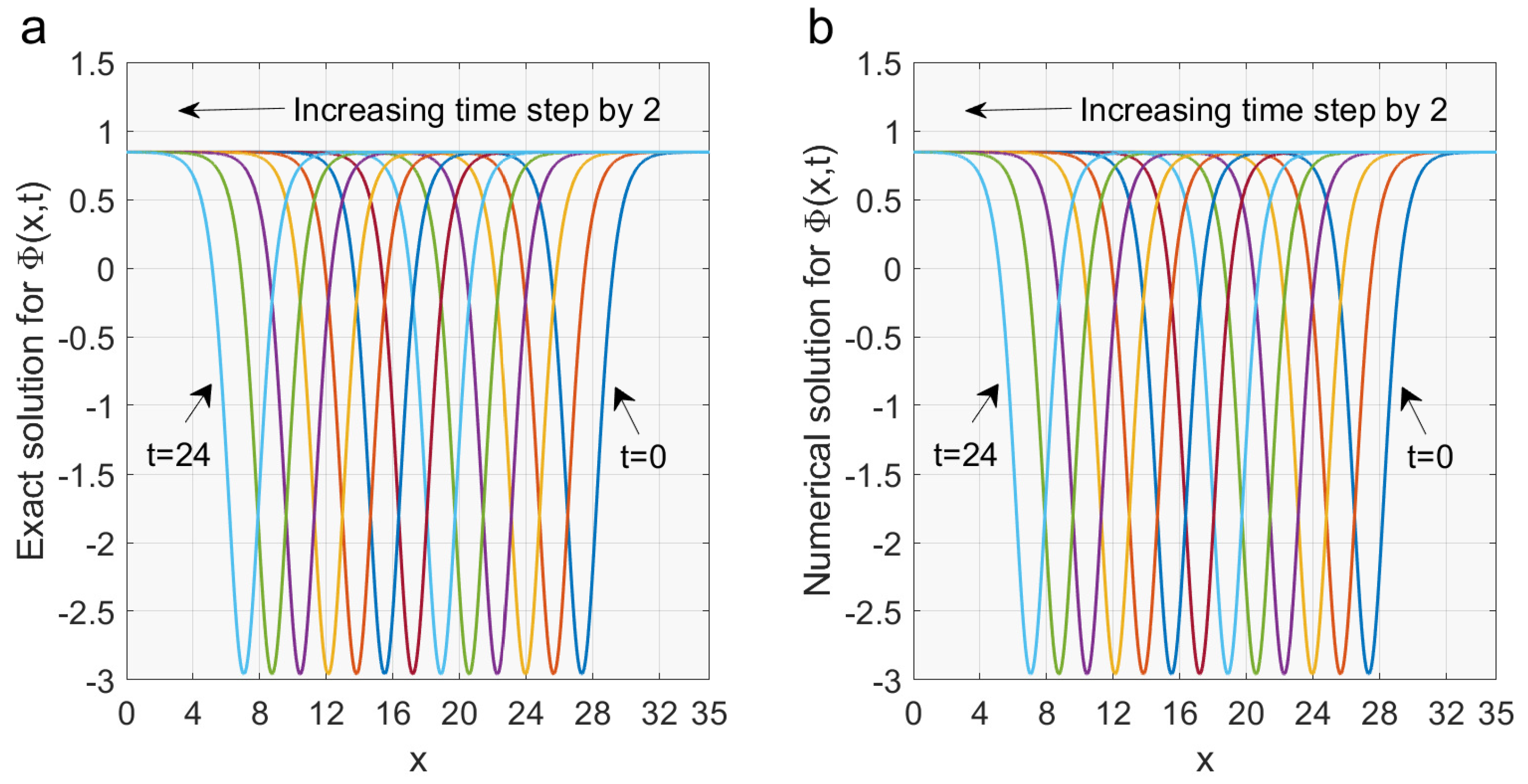
Figure 2.
Figure (a) shows the time evolution of the exact solution of while Figure (b) presents the time evolution of the numerical solution of We consider
Figure 2.
Figure (a) shows the time evolution of the exact solution of while Figure (b) presents the time evolution of the numerical solution of We consider

Figure 3.
Figure (a) shows the time evolution of the exact solution of while Figure (b) presents the time evolution of the numerical solution of We consider
Figure 3.
Figure (a) shows the time evolution of the exact solution of while Figure (b) presents the time evolution of the numerical solution of We consider

Figure 4.
3D figures comparing the performance of the numerical method with the exact solution. The exact solution of (Figure (a)) and the numerical solution of (Figure (b)) are graphically compared in these plots.
Figure 4.
3D figures comparing the performance of the numerical method with the exact solution. The exact solution of (Figure (a)) and the numerical solution of (Figure (b)) are graphically compared in these plots.

Figure 5.
Figure (a) presents a 3D surface for the exact solution of while Figure (b) illustrates a 3D surface for the numerical solution of The numerical graph seems to be identical with the exact one.
Figure 5.
Figure (a) presents a 3D surface for the exact solution of while Figure (b) illustrates a 3D surface for the numerical solution of The numerical graph seems to be identical with the exact one.

Figure 6.
Figure (a) compares some numerical solutions of with the exact solution of for various values of In Figure (b), we present a comparison between the exact and numerical solutions of The numerical solutions of and approach the exact solutions if is very small, as can be observed in these figures.


Table 1.
error and CPU time consumed to arrive at for the numerical process.
| Error for | Error for | CPU | |
|---|---|---|---|
| s | |||
| s | |||
| s | |||
| s | |||
| s | |||
| s |
© 2020 by the authors. Licensee MDPI, Basel, Switzerland. This article is an open access article distributed under the terms and conditions of the Creative Commons Attribution (CC BY) license (http://creativecommons.org/licenses/by/4.0/).
Share and Cite
MDPI and ACS Style
Alharbi, A.; Almatrafi, M.B. Exact and Numerical Solitary Wave Structures to the Variant Boussinesq System. Symmetry 2020, 12, 1473. https://0-doi-org.brum.beds.ac.uk/10.3390/sym12091473
AMA Style
Alharbi A, Almatrafi MB. Exact and Numerical Solitary Wave Structures to the Variant Boussinesq System. Symmetry. 2020; 12(9):1473. https://0-doi-org.brum.beds.ac.uk/10.3390/sym12091473
Chicago/Turabian StyleAlharbi, Abdulghani, and Mohammed B. Almatrafi. 2020. "Exact and Numerical Solitary Wave Structures to the Variant Boussinesq System" Symmetry 12, no. 9: 1473. https://0-doi-org.brum.beds.ac.uk/10.3390/sym12091473
Note that from the first issue of 2016, this journal uses article numbers instead of page numbers. See further details here.