Dynamic Response of the Newton Voigt–Kelvin Modelled Linear Viscoelastic Systems at Harmonic Actions

Abstract

The variety of viscoelastic systems and structures, for the most part, is studied analytically, with significant results. As a result of analytical, numerical and experimental research, which was conducted on a larger variety of linear viscoelastic systems and structures. We analyzed the dynamic behavior for the viscoelastic composite materials, anti-vibration viscous-elastic systems consisting of discrete physical devices, road structures consisting of natural soil structures with mineral aggregates and asphalt mixes, and mixed mechanic systems of insulation of the industrial vibrations consisting of elastic and viscous devices. In this context, the compound rheological model can be schematized as being $V-\left(E|V\right)$ type of the Newton Voigt–Kelvin model with inertial excited mass, applicable to linear viscoelastic materials.

1. Introduction

For some materials, systems and harmonically excited linear viscoelastic structures, the dynamic behavior can be described by the rheological Newton Voigt–Kelvin model.

The dynamic model consists in the fact that the Newton Voigt–Kelvin linear viscoelastic system consists of a mobile mass m driven by an inertial rotational excitation force, named dynamic action F(t), and the fixed basis part that the dynamic action is transmitted to, named transmitted dynamic force Q(t). [1,2,3].

The dynamic analysis of the response highlights the parametric evolution of the amplitudes of the instantaneous displacements, of the transmitted dynamic force and of the dissipated energy in relation to the continuous variation of the excitation pulsation ω or $\mathsf{\Omega }=\frac{\omega }{{\omega }_n}$ and, according to the discrete variation of the linear viscosity parameters c or $\zeta$, where ω_n is the natural pulsation of the system and $\zeta$ is the fraction of the critical amortization so that $c=2\zeta {\omega }_{n}m$.

The families of curves were numerically lifted and experimentally checked on significant domains of technical interest, the specific conclusions being established with the dynamic behavior of the materials, systems and Newton Voigt–Kelvin $V-\left(E|V\right)$ type modelled structured. [4,5].

A high number and are experimentally verified areas of technical interest established specific conclusions consistent with the dynamic behavior of materials, systems and structures modeled with Newton Voigt–Kelvin type V − (E│V). [6,7,8].

2. Dynamic Response at Displacements

The viscoelastic materials that can be modelled by the combination of Newton and Voigt—Kelvin models in series, that is $V-\left(E|V\right)$, are characterized by partial rigidity that reflects the elastic behavior expressed by the rigidity coefficients k, as well as the dissipative viscous behavior expressed by the partial dissipation coefficient c and the global dissipation cM, where M is a real and positive multiplier.

The dynamic model is shown in Figure 1, where $F=F\left(t\right)=F_{0}sin\omega t$ is the disruptive force and $F_0=m_{0}r{\omega }^2$ is the amplitude of disruptive force, c is the linear viscous amortization proportional to the deformation rate of the viscous element, m is the mass, k the rigidity of the Hooke elastic element, and kM is the overall amortization coefficient of the Newton viscous element. [9,10].

The parametric data for an experimental dynamic model are the following: m = 4 × 10³ kg; m₀r = 20 kgm; k = 10⁸ N/m; N = 10; c = (7, 9, 11, 13) × 10⁵ Ns/m; ζ = 0.15; 0.18; 0.22; 0.32; ω = 0 ÷ 500 rad/s; Ω = 0 ÷ 10.

The parametric values represent the result of the statistical processing for a number of over 1200 samples obtained “in situ” by vibration compaction of road structures. Thus, samples were taken from construction sites in Romania on the following highways: Cluj—Napoca—Oradea (Transylvania), Bucharest—Constanta, Timișoara—Deva, Sebeș—Turda. It is mentioned that the soils used on certain parts had a high content of sand (40%), mixed with river mineral aggregates (20%), clay (30%), crushed stone (5%) and stabilizer (5%) [11,12,13,14].

For this composition, as a result of geotechnical tests, the rheological Newton Voigt–Kelvin model was finalized.

The mentioned rheological model was verified at the dynamic compaction, with vibrating rollers of the road structures with asphalt mixtures. Thus, for the mixture recipe of the asphalt cover, which contains an increased dose of bitumen, a good behavior, according to the Newton Voigt–Kelvin model, was found experimentally in the laboratory and “in situ”.

The Newton Voigt–Kelvin linear dynamical system of $V-\left(E|V\right)$ type, with m mass and $x=x\left(t\right)$, $y=y\left(t\right)$ coordinates, has the unidirectional vertical displacement. Dampers have constant c and Mc, and the spring has constant k (Figure 1).

For the system in Figure 1, the movement differential equations, expressed in complex, are as follows [15,16,17]:

$$\{\begin{array}{l}m\ddot{\tilde{x}}+Mc\left(\dot{\tilde{x}}-\dot{\tilde{y}}\right)=F_0{e}^{j\omega t}\\ k\tilde{y}+c\dot{\tilde{y}}=Mc\left(\tilde{\dot{x}}-\tilde{\dot{y}}\right)\end{array}$$

(1)

Solutions $\tilde{x}$ and $\tilde{y}$ are as follows:

• $\tilde{x}=\tilde{X}{e}^{j\omega t}$ with $\dot{\tilde{x}}=j\omega \tilde{X}{e}^{j\omega t}$ and $\ddot{\tilde{x}}=-{\omega }^2\tilde{X}{e}^{j\omega t}$
• $\tilde{y}=\tilde{Y}{e}^{j\omega t}$ with $\dot{\tilde{y}}=j\omega \tilde{Y}{e}^{j\omega t}$

which, inserted in (1), generate an algebraic equation system in $\tilde{X}$ and $\tilde{Y}$, as:

$$\{\begin{array}{c}\left(-m{\omega }^2+jc\omega M\right)\tilde{X}-jc\omega \tilde{Y}=F_0\\ jc\omega M\tilde{X}-\left[k+jc\omega \left(1+M\right)\right]\tilde{Y}=0\end{array}$$

(2)

with the system determinant D, as:

$$D=\left[mk{\omega }^2+c^2{\omega }^2{M}^2\right]-jc\omega \left[Mk-m{\omega }^2\left(1+M\right)\right]$$

or

$$D\left(\zeta ,\mathsf{\Omega }\right)=k^2\left\{\left[{\mathsf{\Omega }}^2+{\left(2\zeta \mathsf{\Omega }\right)}^2{M}^2\right]-j\left(2\zeta \mathsf{\Omega }\right)\left[M-{\mathsf{\Omega }}^2\left(1+\mathrm{M}\right)\right]\right\}$$

Solving system (2), we have:

$$\tilde{X}=F_0\frac{k+jc\omega \left(1+\mathrm{M}\right)}{-\left[mk{\omega }^2+c^2{\omega }^2{M}^2\right]-jc\omega \left[Mk-m{\omega }^2\left(1+M\right)\right]}$$

(3)

Noting in relation (1), with $a_1=k;a_2=c\omega \left(1+M\right);a_3=-\left[mk{\omega }^2+c^2{\omega }^2{M}^2\right];$ $a_4=c\omega \left[Mk-m{\omega }^2\left(1+M\right)\right]$, we have:

$$\tilde{X}=F_0\frac{a_1+j{a}_2}{a_3-j{a}_4}$$

For solution $\tilde{X}$ of system (2), as complex function, with $j=\sqrt{-1}$, we have:

$$\tilde{X}=F_0\frac{1}{a_3^2+a_4^2}\left[\left(a_1{a}_3-a_2{a}_4\right)+j\left(a_2{a}_3+a_1{a}_4\right)\right]$$

Amplitude $\left|\tilde{X}\right|=X_0$ is as follows:

$${\left|\tilde{X}\right|}^2=X_0^2=F_0^2\frac{a_1^2+a_2^2}{a_3^2+a_4^2}$$

For solution

$$X_0\left(c,\omega \right)=F_0\sqrt{\frac{k^2+c^2{\omega }^2{\left(1+M\right)}^2}{{\left[km{\omega }^2+c^2{\omega }^2{M}^2\right]}^2+c^2{\omega }^2{\left[Mk-m{\omega }^2\left(1+M\right)\right]}^2}}$$

(4)

and in relative measures $\mathsf{\Omega }$ and $\zeta$, we have:

$$X_0\left(\zeta ,\mathsf{\Omega }\right)=\frac{F_0}{k}\sqrt{\frac{1+{\left(2\zeta \mathsf{\Omega }\right)}^2{\left(1+M\right)}^2}{{\left[{\mathsf{\Omega }}^2+{\left(2\zeta \mathsf{\Omega }\right)}^2{M}^2\right]}^2+{\left(2\zeta \mathsf{\Omega }\right)}^2{\left[M-{\mathsf{\Omega }}^2\left(1+M\right)\right]}^2}}$$

(5)

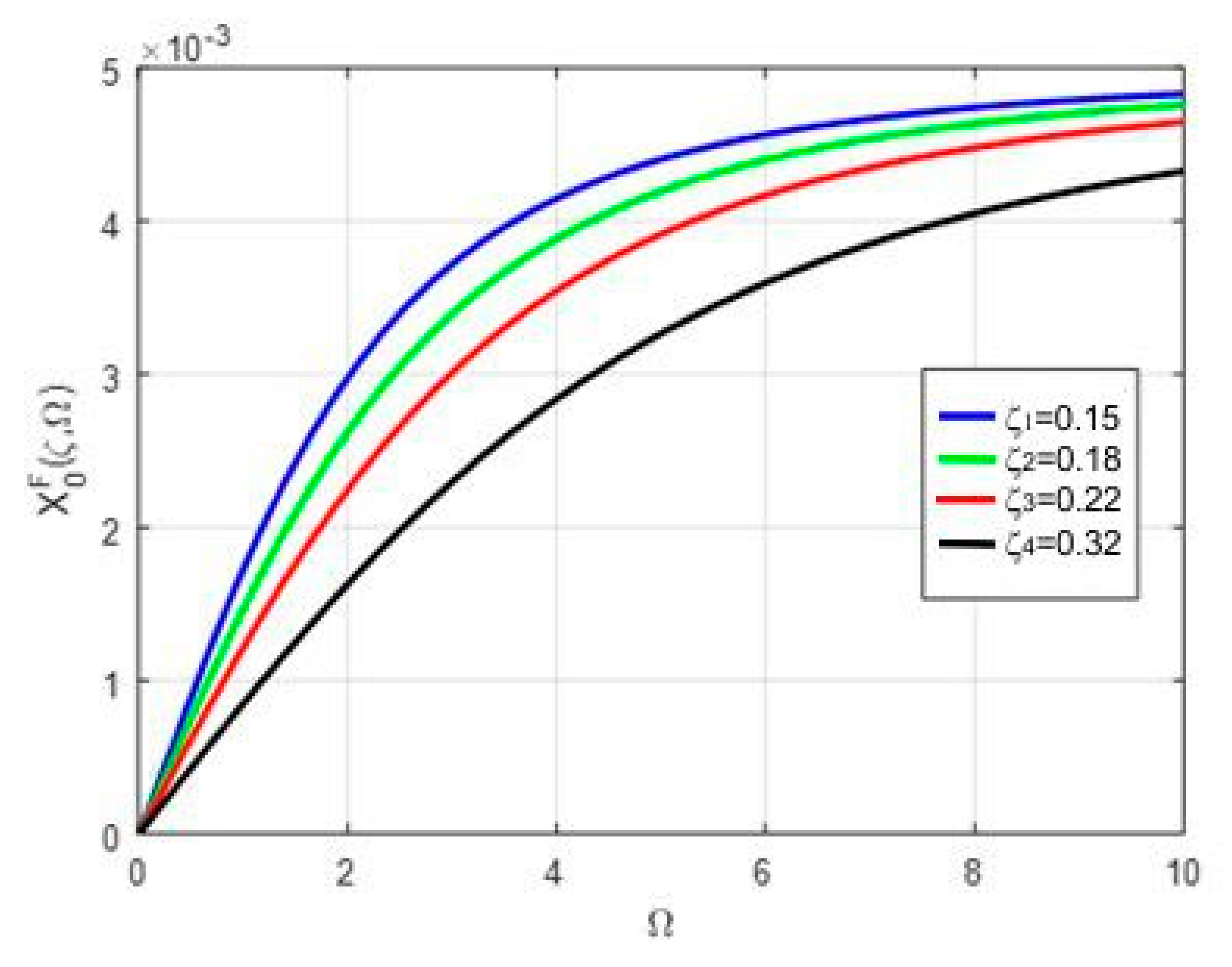
Figure 2 presents the curve families $X_0\left(\zeta ,\mathsf{\Omega }\right)$ for force $F_0=m_{0}r{\omega }^2\equiv \frac{m_{0}r}{m}k{\mathsf{\Omega }}^2$.

The boundary conditions for the family of curves in Figure 2 are as follows:

• for $\mathsf{\Omega }\to 0$ we have $\underset{\mathsf{\Omega }\to 0}{\lim }{X}_0\left(\zeta ,\mathsf{\Omega }\right)$
• for $\mathsf{\Omega }\to \infty$ we have $\underset{\mathsf{\Omega }\to 0}{\lim }{X}_0\left(\zeta ,\mathsf{\Omega }\right)=\frac{m_{0}r}{m}$

which is reflected for all curves in Figure 2.

For solution $\tilde{Y}$ of the system (2), as complex function, with $j=\sqrt{-1}$, we have:

$$\tilde{Y}=F_0\frac{jc\omega M}{\left[km{\omega }^2+c^2{\omega }^2{M}^2\right]-jc\omega \left[Mk-m{\omega }^2\left(1+M\right)\right]}$$

(6)

where we note $\alpha =0,$ $\beta =c\omega M$, $\delta =c\omega \left[Mk-m{\omega }^2\left(1+M\right)\right]$, $\gamma =-\left[km{\omega }^2+c^2{\omega }^2{M}^2\right]$, $G={\gamma }^2+{\delta }^2$. Thus, we have:

$$\tilde{Y}=F_0\frac{1}{{\gamma }^2+{\delta }^2}\left[\beta \delta +j\beta \gamma \right]$$

(7)

with amplitude $Y_0$ as:

$${\left|\tilde{Y}\right|}^2=Y_0^2=F_0^2\frac{{\beta }^2}{{\gamma }^2+{\delta }^2}$$

For solution

$$Y_0=F_0\frac{\beta }{\sqrt{{\gamma }^2+{\delta }^2}}$$

In natural measure, we have $Y_0\left(c,\omega \right)$ as:

$$Y_0\left(c,\omega \right)=F_0\frac{c\omega M}{\sqrt{{\left[km{\omega }^2+c^2{\omega }^2{M}^2\right]}^2+c^2{\omega }^2{\left[Mk-m{\omega }^2\left(1+M\right)\right]}^2}}$$

(8)

For the solution in relative measures, it can be written:

$$Y_0\left(\zeta ,\mathsf{\Omega }\right)=\frac{F_0}{k}\frac{\left(2\zeta \mathsf{\Omega }\right)M}{\sqrt{{\left[{\mathsf{\Omega }}^2+{\left(2\zeta \mathsf{\Omega }\right)}^2{M}^2\right]}^2+{\left(2\zeta \mathsf{\Omega }\right)}^2{\left[M-{\mathsf{\Omega }}^2\left(1+M\right)\right]}^2}}$$

(9)

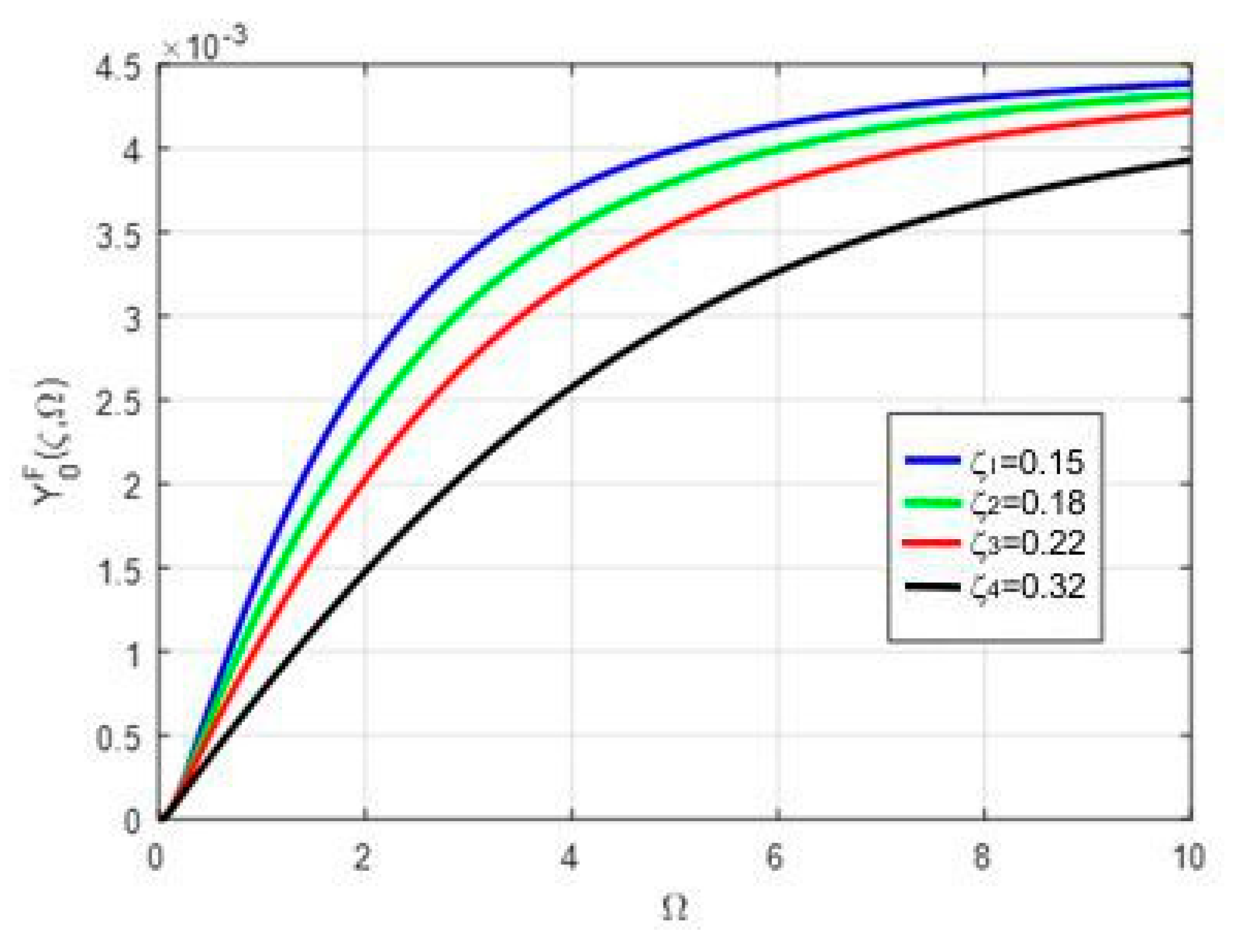
The graphical representation of amplitude $Y_0\left(\zeta ,\mathsf{\Omega }\right)$ for $F_0=m_{0}r{\omega }^2\equiv \frac{m_{0}r}{m}k{\mathsf{\Omega }}^2$ is given in Figure 3.

From the analysis of the response in harmonic regime it is found that $Y_0\left(\zeta ,\mathsf{\Omega }\right)$ is the amplitude of the kinematic excitation of the Voigt–Kelvin model.

3. Transmitted Dynamic Force

The transmitted force at fix support is $\tilde{Q}$, as:

$$\tilde{Q}=k\tilde{y}+c\dot{\tilde{y}}$$

For solution

$$\tilde{Q}=\left(k+jc\omega \right)\tilde{Y}{e}^{j\omega t}$$

where $\tilde{Q}=\tilde{Q}\left(t\right)$ is the expression in complex form of the force transmitted to the support.

Introducing $\tilde{Q}$ in relation (7) and use the previous notes, where $c\omega =\frac{1}{M}\beta$, we have:

$$\tilde{Q}=F_0\frac{\beta }{{\gamma }^2+{\delta }^2}\left[\left(k\delta -\frac{1}{M}\beta \gamma \right)+j\left(k\gamma +\frac{1}{M}\beta \delta \right)\right]$$

(10)

with amplitude $Q_0$ as:

$$Q_0=\beta F_0\sqrt{\frac{k^2{M}^2+{\beta }^2}{G{M}^2}}$$

(11)

Returning to natural parameters, we have:

$$\begin{gathered} Q_0\left(c,\omega \right)=F_0\frac{c\omega M\sqrt{k^2+c^2{\omega }^2}}{\sqrt{{\left[km{\omega }^2+c^2{\omega }^2{M}^2\right]}^2+c^2{\omega }^2{\left[Mk-m{\omega }^2\left(1+M\right)\right]}^2}} \\ =F_0\frac{c\omega M\sqrt{k^2+c^2{\omega }^2}}{\sqrt{G}} \end{gathered}$$

(12)

For solution in relative measures, relation (12) is as:

$$Q_0\left(\zeta ,\mathsf{\Omega }\right)=F_0\frac{\left(2\zeta \mathsf{\Omega }\right)M\sqrt{1+{\left(2\zeta \mathsf{\Omega }\right)}^2}}{\sqrt{{\left[{\mathsf{\Omega }}^2+{\left(2\zeta \mathsf{\Omega }\right)}^2{M}^2\right]}^2+{\left(2\zeta \mathsf{\Omega }\right)}^2{\left[M-{\mathsf{\Omega }}^2\left(1+M\right)\right]}^2}}=F_0\frac{\left(2\zeta \mathsf{\Omega }\right)M\sqrt{1+{\left(2\zeta \mathsf{\Omega }\right)}^2}}{\sqrt{H}}$$

(13)

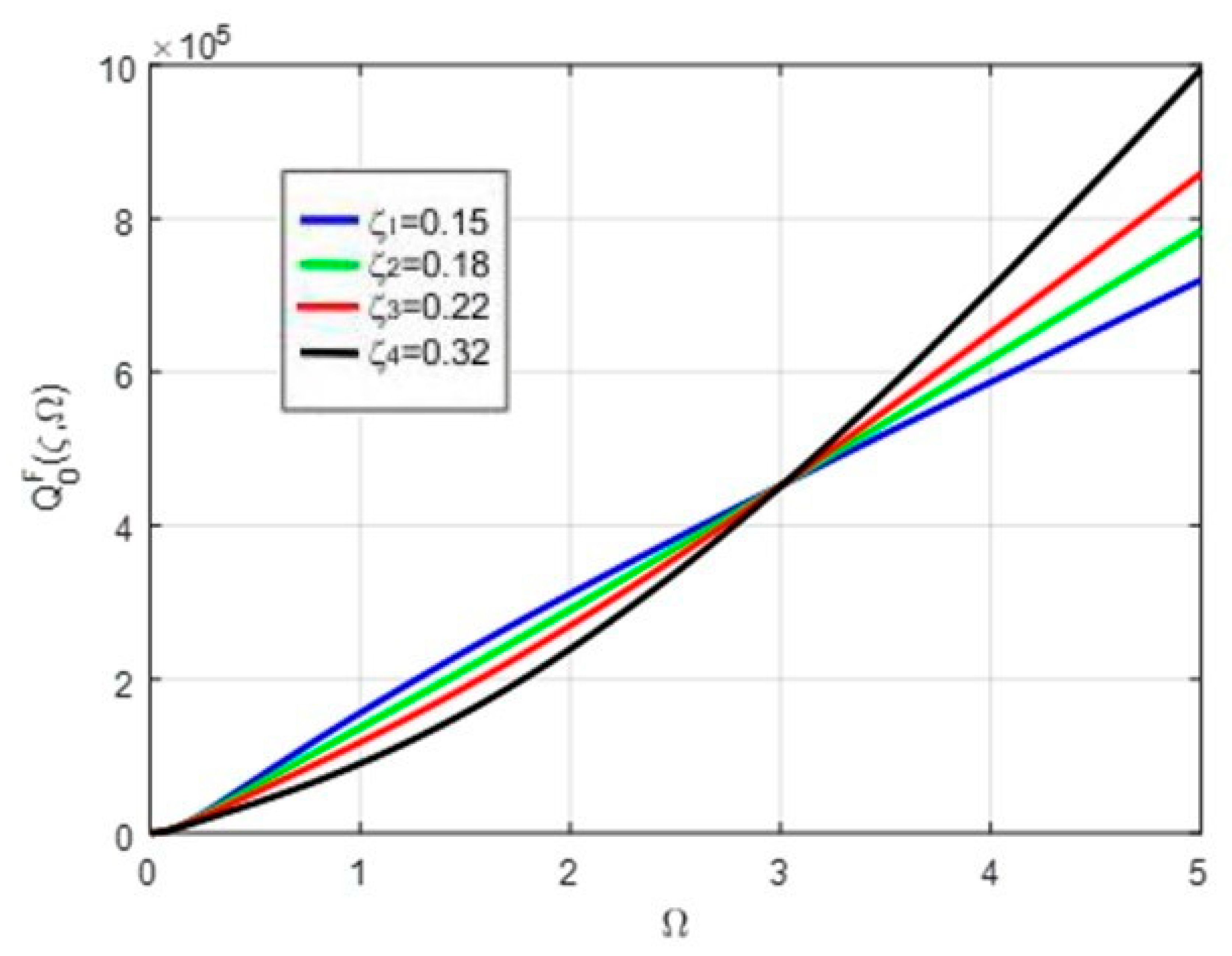
with representation in Figure 4.

The following notes were used:

$$G={\left[km{\omega }^2+c^2{\omega }^2{M}^2\right]}^2+c^2{\omega }^2{\left[Mk-m{\omega }^2\left(1+M\right)\right]}^2$$

(14)

$$H={\left[{\mathsf{\Omega }}^2+{\left(2\zeta \mathsf{\Omega }\right)}^2{M}^2\right]}^2+{\left(2\zeta \mathsf{\Omega }\right)}^2{\left[M-{\mathsf{\Omega }}^2\left(1+M\right)\right]}^2$$

(15)

so that G and H are in the following relation:

$$G=k^{4}H$$

(16)

4. Dynamic Insulation Capacity

In this case, the dynamic transmissibility may be defined as:

$$T=\frac{Q_0}{F_0}$$

Taking into account relations (12) and (13), the calculation formulas emerge as:

$$T_0\left(c,\omega \right)=\frac{c\omega M\sqrt{k^2+c^2{\omega }^2}}{{\left[km{\omega }^2+c^2{\omega }^2{M}^2\right]}^2+c^2{\omega }^2{\left[Mk-m{\omega }^2\left(1+M\right)\right]}^2}$$

(17)

$$T_0\left(\zeta ,\mathsf{\Omega }\right)=\frac{\left(2\zeta \mathsf{\Omega }\right)M\sqrt{1+{\left(2\zeta \mathsf{\Omega }\right)}^2}}{\sqrt{{\left[{\mathsf{\Omega }}^2+{\left(2\zeta \mathsf{\Omega }\right)}^2{M}^2\right]}^2+{\left(2\zeta \mathsf{\Omega }\right)}^2{\left[M-{\mathsf{\Omega }}^2\left(1+M\right)\right]}^2}}$$

(18)

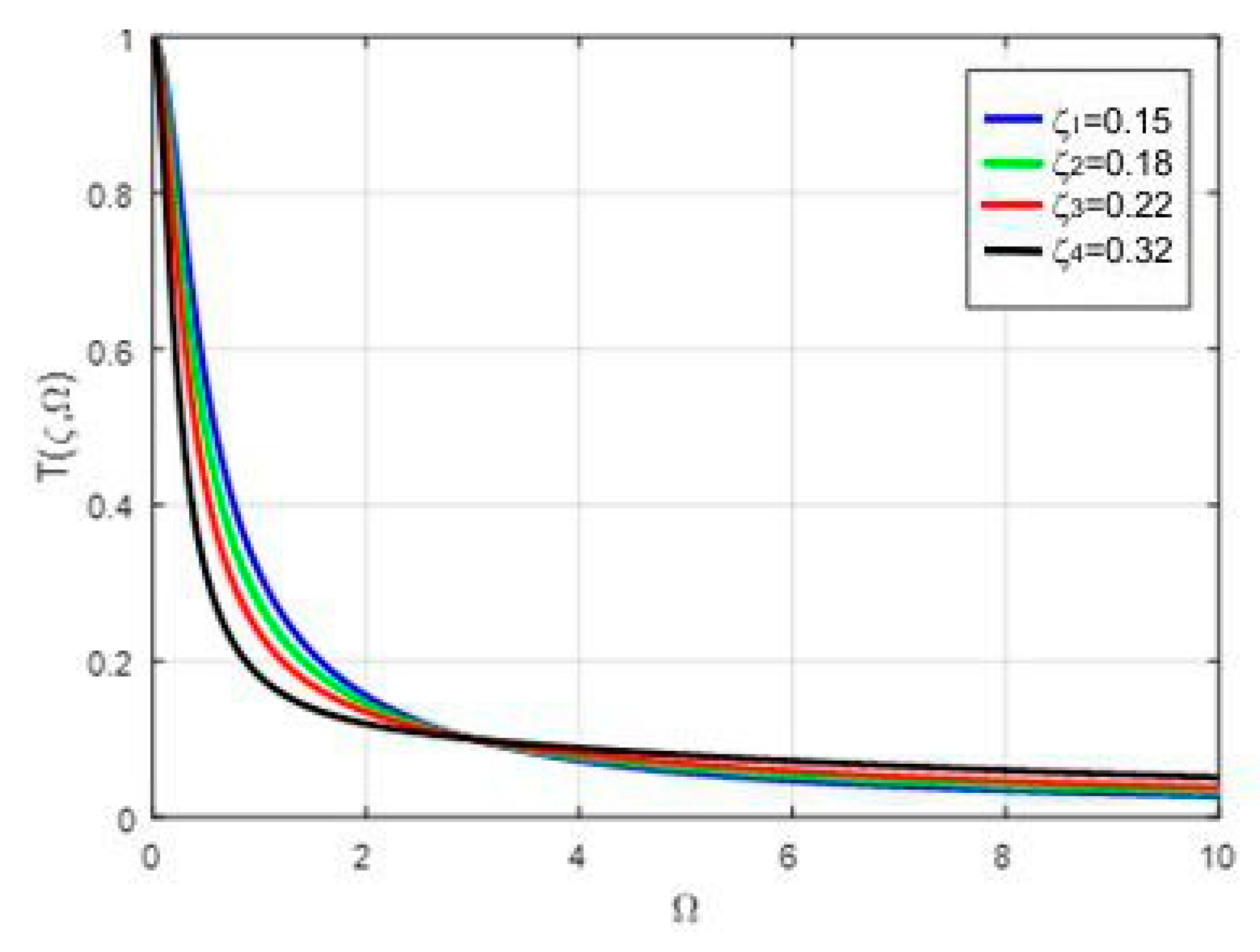
with representation in Figure 5.

5. Deformation of Damper Systems

(a) For the damper with multiplied M viscous characteristic, that is in the case of the amortization constant cM, the instantaneous deformation is [18,19,20]:

$$\tilde{v}=\tilde{x}-\tilde{y}=\left(\tilde{X}-\tilde{Y}\right)e^{j\omega t}$$

By replacing $\tilde{X}$ in relation (7.165) and $\tilde{Y}$ in relation (7.168), with the specification that $\tilde{v}$ may be written as:

$$\tilde{v}={\tilde{V}}_0{e}^{j\omega t}$$

(19)

we can obtain the amplitude of deformation $V_0$, as follows:

$${\tilde{V}}_0=\tilde{X}-\tilde{Y}$$

(20)

and in the end:

$$V_0=F_0\sqrt{\frac{k^2+c^2{\omega }^2}{a_3^2+a_4^2}}$$

(21)

from which

$$V_0\left(c,\omega \right)=F_0\sqrt{\frac{k^2+c^2{\omega }^2}{G}}$$

(22)

For solution in relative measures, as follows:

$$V_0\left(\zeta ,\mathsf{\Omega }\right)=\frac{F_0}{k}\sqrt{\frac{1+{\left(2\zeta \mathsf{\Omega }\right)}^2}{H}}$$

(23)

(b) For damper c, the instantaneous deformation is the same as the instantaneous displacement $\tilde{y}$. The maximum deformation (amplitude) is $Y_0$, given by relation (8) for solution (9) were we use the previous notes $\beta ,\gamma ,\delta$. Thus, we have:

$$Y_0\left(c,\omega \right)=F_0\frac{c\omega M}{\sqrt{G}}$$

(24)

$$Y_0\left(\zeta ,\mathsf{\Omega }\right)=\frac{F_0}{k}\frac{\left(2\zeta \mathsf{\Omega }\right)M}{\sqrt{H}}$$

(25)

6. Dissipated Energy

For the studied model, the dissipated energy on cycle is as:

$$W_d=W_d^I+W_d^{II}$$

where $W_d^I=\pi c\omega Y_0^2$ is the dissipated energy for the constant damper c; $W_d^{II}=\pi Mc\omega V_0^2$—the dissipated energy on the damper with the amortization multiplication Mc. [21,22].

Taking into account relations (20) and (24), energy on cycle may be expressed as:

$$W_d\left(c,\omega \right)=\frac{\pi c\omega }{G}{F}_0^{2}M\left[k^2+c^2{\omega }^2\left(1+M\right)\right]$$

(26)

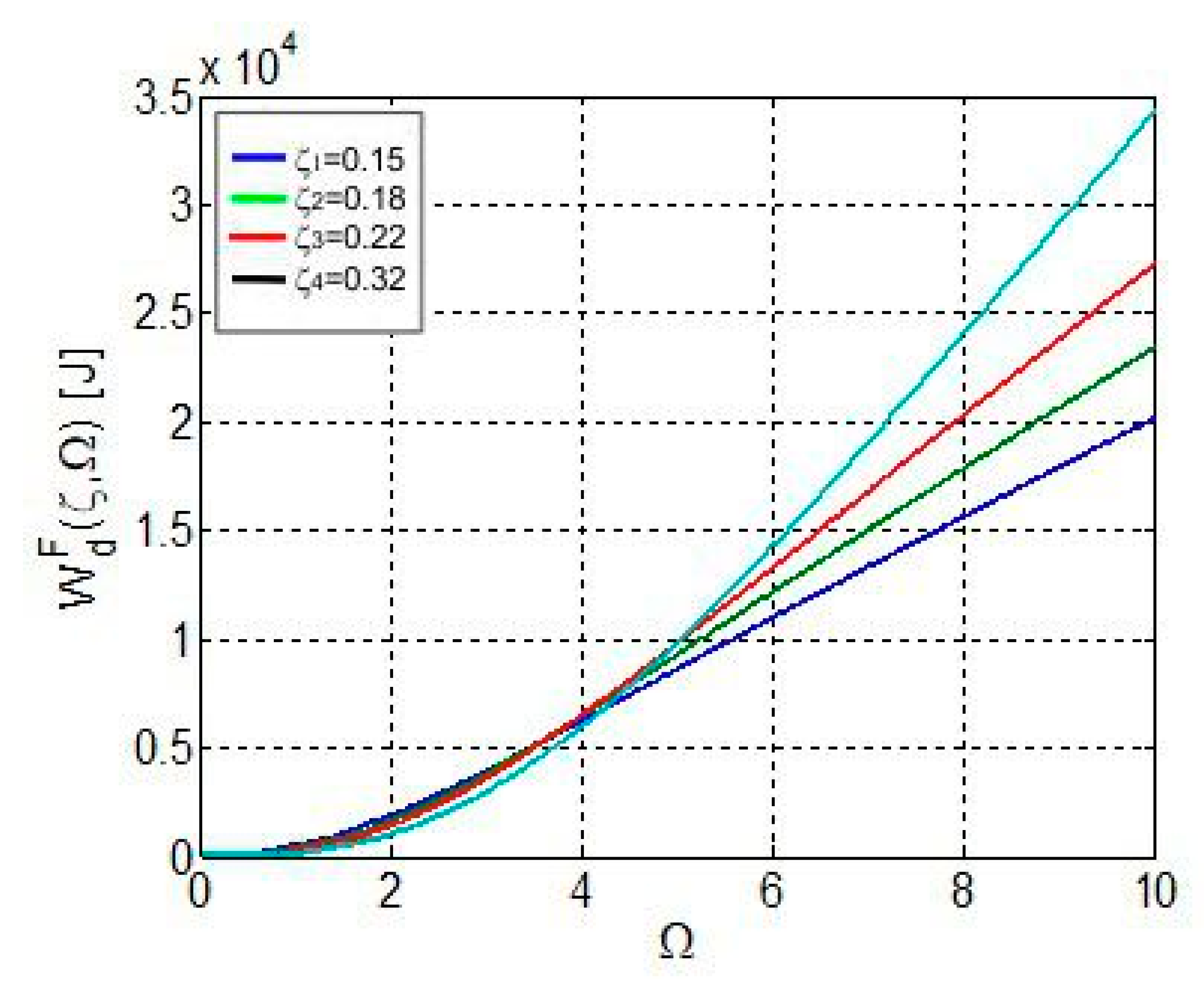
Taking into account that $F_0=m_{0}r{\omega }^2\equiv \frac{m_{0}r}{m}k{\mathsf{\Omega }}^2$, in relative measures, relation (26) becomes:

$$W_d^F\left(\zeta ,\mathsf{\Omega }\right)=\frac{\pi \left(2\zeta \mathsf{\Omega }\right)}{kH}{F}_0^{2}M\left[1+{\left(2\zeta \mathsf{\Omega }\right)}^2\left(1+M\right)\right]$$

(27)

with a graphical representation in Figure 6.

7. Conclusions

The Newton Voigt–Kelvin linear viscoelastic model can be used to study the dynamic behavior of technologically made materials, systems and structures, having the role both to ensure predictable values of the dynamic forces transmitted to the basis as well as to assess the dissipated energy. Based on some anti-vibration devices, favorably assembled for the realization of the Zener linear model, we studied and established solutions for dynamic insulation of the industrial vibrations for dynamic equipment in technological flows at working frequencies between 20 Hz and 50 Hz. [23,24,25].

Additionally, by compacting with vibratory rollers, for certain categories of stratifications of road structures, dynamic behaviors were identified according to the Newton Voigt–Kelvin linear model.

The numerical and experienced dynamic analysis for some categories of engineering applications, enabled the adaptation of a Newton Voigt–Kelvin rheological model, with mass and harmonic excitation with inertial rotating force.

The advantage of the proposed model is that, for composite materials containing structural components with significantly increased viscosity compared to elastic components, the dynamic response is more accurate and precise. Additionally, the shape of the representative curves is sometimes very different from other composite viscoelastic models.

The establishment of the calculation relations and the parametric graphical representation with the identification of the dynamic regimes enable an eloquent evaluation of the dynamic process in its significant evolution. Thus, based on the substantiation of the calculation relations and of the parametric evaluation of the families of lifted curves for a structural multilayer road system compacted with a Bomag vibrating roller, the following conclusions can be summarized [26,27]:

(a) Amplitudes X₀ and Y₀ highlight the maximum displacements of mass m and, respectively, of the viscoelastic component (c, k) in connection with the viscous component (Mc), being useful in the evaluation of the technological parameters;

(b) The families of curves of amplitudes X₀ and Y₀ represented in relation to the relative parameters ζ and Ω highlight the parametric distribution according to the dynamic excitation regimes according to the variation of Ω;

(c) The dynamic area of interest for the stable behavior of the technological vibrations is specific to the domain for which amplitudes tend towards stable asymptotic values for Ω > 8; thus, at significantly high values of the excitation pulsation, under conditions of predictable amortization, amplitudes X₀ and Y₀ present a stable level at small variations in the excitation pulsation [28];

(d) The maximum transmitted dynamic force Q₀ in the post-resonance domain for ω >> ωn. For solution Ω >> 1, present monotonically increasing values depending on the pulsation and the dimension of the viscous amortization;

(e) Transmissibility is decreasing at high values of the excitation pulsation, at discrete variation in the amortization;

(f) The dissipated energy is increasing, depending on the post-resonance variation of the excitation pulsation and the discrete increase in the amortization.

Consequently, based on the physical and mechanical parameters specific to the equivalent Newton Voigt–Kelvin rheological model for materials, systems and viscoelastic structures, we can assess the parametric measures of the dynamic response and of the behavior in the harmonic excitation regime with harmonic rotation forces.

The experimental results performed in the laboratory, and “in situ” in Romania, mostly included in the works cited above [23,26,27,28], as well as the laboratory results presented in the works [24,25,29,30], highlighted the importance of adopting the Newton Voigt–Kelvin model, for specified materials compared to other viscoelastic composite models.

References

- Bratu, P. Evaluation of the Dissipated Energy for Viscoelastic and Hysteretic Soil Systems for Road Works; Test Report for Bechtel company—“Transylvania Highway”; ICECON SA: Bucharest, Romania, 2012. [Google Scholar]
- Bratu, P. Dynamic Stress Dissipated Energy Rating of Materials with Maxwell Rheological Behaviour. Appl. Mech. Mater. 2015, 801, 115–121. [Google Scholar] [CrossRef]
- Bratu, P. The Behaviour of Nonlinear Viscoelastic Systems Subjected to Harmonic Dynamic Excitation. In Proceedings of the 9th International Congress on Sound and Vibration, University of Central Florida Orlando, Orlando, FL, USA, 8–11 July 2002. [Google Scholar]
- Bratu, P. Dynamic response of nonlinear systems under stationary harmonic excitation. In Proceedings of the Non-Linear Acoustics and Vibration, 11th International Congress on Sound and Vibration, St. Petersburg, Russia, 5–8 July 2004; pp. 2767–2770. [Google Scholar]
- Bratu, P. Dynamic analysis in case of compaction vibrating rollers intended for road works. In Proceedings of the 17th International Congress on Sound& Vibration, ICSV, Cairo, Egypt, 18–22 July 2010. [Google Scholar]
- Bratu, P.; Stuparu, A.; Popa, S.; Iacob, N.; Voicu, O. The Assessment of the Dynamic Response to Seismic Excitation for Constructions Equipped with Base Isolation Systems According to the Newton-Voigt-Kelvin Model. Acta Tech. Napoc. Ser. Appl. Math. Eng. 2017, 60, 459–464. [Google Scholar]
- Bratu, P.; Stuparu, A.; Leopa, A.; Popa, S. The Dynamic Analyses of a Construction with the Base Insulation Consisting in Anti-Seismic Devices Modelled as a Hooke-Voigt-Kelvin Linear Rheological System. Acta Tech. Napoc. Ser. Appl. Math. Eng. 2018, 60, 465–472. [Google Scholar]
- Bratu, P.; Stuparu, A.; Popa, S.; Iacob, N.; Voicu, O.; Iacob, N.; Spanu, G. The Dynamic Isolation Performances Analysis of the Vibrating Equipment with Elastic Links to a Fixed Base. Acta Tech. Napoc. Ser. Appl. Math. Eng. 2018, 61, 23–28. [Google Scholar]
- Bratu, P. Hysteretic Loops in Correlation with the Maximum Dissipated Energy, for Linear Dynamic Systems. Symmetry 2019, 11, 315. [Google Scholar] [CrossRef] [Green Version]
- Bratu, P.; Dobrescu, C.F. Dynamic Response of Zener-Modelled Linearly Viscoelastic Systems under Harmonic Excitation. Symmetry 2019, 11, 1050. [Google Scholar] [CrossRef] [Green Version]
- Bratu, P.; Buruga, A.; Chilari, O.; Ciocodeiu, A.; Oprea, I. Evaluation of the Linear Viscoelastic Force for a Dynamic System (m, c, k) Excited with a Rotating Force. RJAV 2019, 16, 39–46. [Google Scholar]
- Dobrescu, C.F. Analysis of the dynamic regime of forced vibrations in the dynamic compacting process with vibrating roller. Acta Tech. Napoc. Appl. Math. Mech. Eng. 2019, 62, 71–76. [Google Scholar]
- Dobrescu, C.F. Highlighting the Change of the Dynamic Response to Discrete Variation of Soil Stiffness in the Process of Dynamic Compaction with Roller Compactors Based on Linear Rheological Modelling. In Acoustics & Vibration of Mechanical Structures II; Herisanu, N., Marinca, V., Eds.; [ISI Web of Science (WoS)]; Trans Tech Publications Ltd.: Freienbach, Switzerland, 2015; Volume 801, pp. 242–248. ISBN 978-3-03835-628-8. [Google Scholar] [CrossRef]
- Dobrescu, C.F.; Brăguţă, E. Optimization of Vibro-Compaction Technological Process. Considering Rheological Properties. In Proceedings of the 14th AVMS Conference, Timisoara, Romania, 25–26 May 2017; Nicolae, H., Vasile, M., Eds.; Springer: Berlin/Heidelberg, Germany; pp. 287–293. [Google Scholar] [CrossRef]
- Morariu-Gligor, R.M.; Crisan, A.V.; Şerdean, F.M. Optimal Design of a One-Way Plate Compactor. Acta Tech. Napoc. Ser. Appl. Math. Mech. Eng. 2017, 60, 557–564. [Google Scholar]
- Mooney, M.A.; Rinehart, R.V. Field Monitoring of Roller Vibration during Compaction of Subgrade Soil. J. Geotech. Geoenviron. Eng. ASCE 2007, 133, 257–265. [Google Scholar] [CrossRef]
- Mooney, M.A.; Rinehart, R.V. In-Situ Soil Response to Vibratory Loading and Its Relationship to Roller-Measured Soil Stiffness. J. Geotech. Geoenviron. Eng. ASCE 2009, 135, 1022–1031. [Google Scholar] [CrossRef] [Green Version]
- Vucetic, M.; Dobry, R. Effect of Soil Elasticity on Cyclic Response. J. Geotech. Eng. 1991, 117, 89–107. [Google Scholar] [CrossRef]
- Wersäll, C.; Larsson, S.; Bodare, A. Dynamic Response of Vertically Oscillating Foundation At. large Strain. In Proceedings of the 14th International Conference of the International Association for Computer Methods and Advances in Geomechanics, Kyoto, Japan, 22–25 September 2014; pp. 643–647. [Google Scholar]
- Wersäll, C.; Larsson, S.; Ryden, N.; Nordfeld, I. Frequency Variable Surface Compaction of Sand Using Rotating Mass Oscillators. Geotech. Test. J. 2015, 38, 1–10. [Google Scholar] [CrossRef]
- Wersäll, C.; Nordfeld, I.; Larsson, S. Soil Compaction by Vibratory Roller with Variable Frequency; Submitted to Geotechnics for Sustainable Infrastructure Development—Geotech: Hanoi, Vietnam; Available online: https://geotechn.vn/geotec-hanoi-rewind/geotec-hanoi-2016/ (accessed on 24 November 2016).
- Yoo, T.-S.; Selig, E.T. Dynamics of Vibratory Roller Compaction. J. Geotech. Eng. Div. 1979, 105, 1211–1231. [Google Scholar]
- ICECON. Test. Report for Laboratory and “In Situ” Tests Performed on the Road Layers of the Bucureşti-Constanța Highway; ICECON: Bucharest, Romania, 2004. [Google Scholar]
- Lucas, E.F.; Soares, B.G.; Monteiro, E. Caracterização de Polimeros; e-Papers: Rio de Janeiro, Brazil, 2001. [Google Scholar]
- Gedde, U.W. Polymer Physics; Kluver: Dordrecht, The Netherlands; Boston, MA, USA; London, UK, 2001. [Google Scholar]
- ICECON. Test. Report for Laboratory and “In Situ” Tests for the Lugoj-Deva Highway; ICECON: Bucharest, Romania, 2015. [Google Scholar]
- ICECON. Test. Report for Laboratory and “In Situ” Tests for the Timisoara-Lugoj Highway; ICECON: Bucharest, Romania, 2016. [Google Scholar]
- ICECON. Test. Report for Laboratory and “In Situ” Tests. Transylvania Highway, Bechtel Romania; ICECON: Bucharest, Romania, 2008. [Google Scholar]
- Menard, K.P. Dynamic Mechanical Analysis: An. Introduction, 2nd ed.; CRC Press: Boca Raton, FL, USA, 2008. [Google Scholar]
- Brostow, W.; Hagg Lobland, H.E. Materials: Introduction and Applications; John Wiley & Sons: Hoboken, NJ, USA, 2017. [Google Scholar]
Figure 1.
Newton Voigt–Kelvin model with harmonically excited mass.
Figure 2.
Curves family , in m, for force .
Figure 3.
Figure 4.
Curves family for force .
Figure 5.
Curves family .
Figure 6.
Curves family of the dissipated energy on cycle .
© 2020 by the author. Licensee MDPI, Basel, Switzerland. This article is an open access article distributed under the terms and conditions of the Creative Commons Attribution (CC BY) license (http://creativecommons.org/licenses/by/4.0/).
Share and Cite
MDPI and ACS Style
Dobrescu, C. Dynamic Response of the Newton Voigt–Kelvin Modelled Linear Viscoelastic Systems at Harmonic Actions. Symmetry 2020, 12, 1571. https://0-doi-org.brum.beds.ac.uk/10.3390/sym12091571
AMA Style
Dobrescu C. Dynamic Response of the Newton Voigt–Kelvin Modelled Linear Viscoelastic Systems at Harmonic Actions. Symmetry. 2020; 12(9):1571. https://0-doi-org.brum.beds.ac.uk/10.3390/sym12091571
Chicago/Turabian StyleDobrescu, Cornelia. 2020. "Dynamic Response of the Newton Voigt–Kelvin Modelled Linear Viscoelastic Systems at Harmonic Actions" Symmetry 12, no. 9: 1571. https://0-doi-org.brum.beds.ac.uk/10.3390/sym12091571
Note that from the first issue of 2016, this journal uses article numbers instead of page numbers. See further details here.