Dynamics of Nonlocal Rod by Means of Fractional Laplacian

Abstract

The use of fractional models to analyse nonlocal behaviour of solids has acquired great importance in recent years. The aim of this paper is to propose a model that uses the fractional Laplacian in order to obtain the equation ruling the dynamics of nonlocal rods. The solution is found by means of numerical techniques with a discretisation in the space domain. At first, the proposed model is compared to a model that uses Eringen’s classical approach to derive the differential equation ruling the problem, showing how the parameters used in the proposed fractional model can be estimated. Moreover, the physical meaning of the model parameters is assessed. The model is then extended in dynamics by means of a discretisation in the time domain using Newmark’s method, and the responses to different dynamic conditions, such as an external load varying with time and free vibrations due to an initial deformation, are estimated, showing the difference of behaviour between the local response and the nonlocal response. The obtained results show that the proposed model can be used efficiently to estimate the response of the nonlocal rod both to static and dynamic loads.

1. Introduction

Classical elasticity theory assumes that the stress at a point depends only on the displacements in the neighbourhood of the point itself. The results obtained are coherent and meaningful when dealing with structural elements at the macro-scale, i.e., in which the dimensions are much larger than the scale of elementary material particles. However, at the micro-scale, the classical theory of elasticity may be not adequate to estimate the response of solids. In particular, when dealing with elements at the micro-scale, and in order to avoid formulating the problem in the context of lattice theory, several authors prefer to work within the framework of continuum mechanics by introducing the theory of nonlocal elasticity, the roots of which can be traced to the work of Eringen and Edelen [1]. As an example, Bazant [2] showed how the damage may be considered a nonlocal phenomenon, while in [3] it is shown that the effect of the micro-structure can be relevant in the case of wave dispersion in one-dimensional solid. Moreover, in [4] it is shown that nonlocality can arise also at the meso-scale when dealing with composite material.

The main assumption of the nonlocal approach is that, differently from the theory of local elasticity, the stress at a point depends not only on the displacements around the point but also on displacements of points further away. There are several approaches that can be used [5]; for example, the stress may depend on the strains of the whole continuum in an integral form through an appropriate kernel [6]. A differential equation involving the stress and its’ second derivative can be used [7], which can be enriched to deal with nanomaterials [8,9]. More recently, the peridynamic model has been proposed [10], which relates the derivative of stress to an integral involving difference of displacements through a (peridynamic) kernel. The nonlocal elasticity theory allows to study the behaviour of beams at the nano-scale [11,12], also considering the Timoshenko model [13,14,15], the presence of viscoelastic foundation [16], the response to stochastic actions [17,18,19], and allows considering plane elements at the nano-scale [20,21]. A variational approach can also be used [22] and the effect of boundary conditions on the vibration of the beam can be evaluated [23,24].

Another approach to deal with nonlocal elasticity is to use the fractional calculus [25,26]. Within this field, a model based on the fractional Laplacian operator has been proposed in [27], which considered the response of a rod to external load in statics, with a sensibility analysis of the parameter of the model performed in [28]. An application of the fractional calculus to the nonlocal elasticity is in the field of the propagation of waves in nanostructures, for example, to model the dispersion law [29]. A peculiar approach is to model the nonlocal effects by means of long-range interactions of volume elements, as shown in [30,31].

In the present paper, we propose to model the dynamics of a rod by means of the fractional Laplacian operator. In particular, the formulation of the problem is given in [32], where the response in free vibration has been evaluated. In the present paper, we study the response in forced and free oscillation. In Section 2, the main characteristics of the fractional Laplacian model and of the local/nonlocal differential model are recalled. The latter is based on Eringen’s one and allows finding a closed-form response, which is used to discuss the choice of parameters of the fractional Laplacian model. Moreover, in Section 2.3 an approach, by means of fractional Laplacian model, to estimate the response in dynamics is proposed, while Section 2.4 is dedicated to describing the numerical approximation of fractional Laplacian problems. In Section 3 the response to an external excitation is evaluated both for the fractional Laplacian model and the local/nonlocal differential model. In Section 3.3 the solution in dynamics is evaluated by means of discretisation in time domain using Newmark’s method, which allows a rather straightforward and costly effective solution. In Section 4, a short discussion and conclusions are reported.

2. Materials and Methods

2.1. The Fractional Laplacian Model

In [27], a model for a nonlocal rod based on a fractional Laplacian was proposed. In the present section, we recall briefly the main hypothesis and the results.

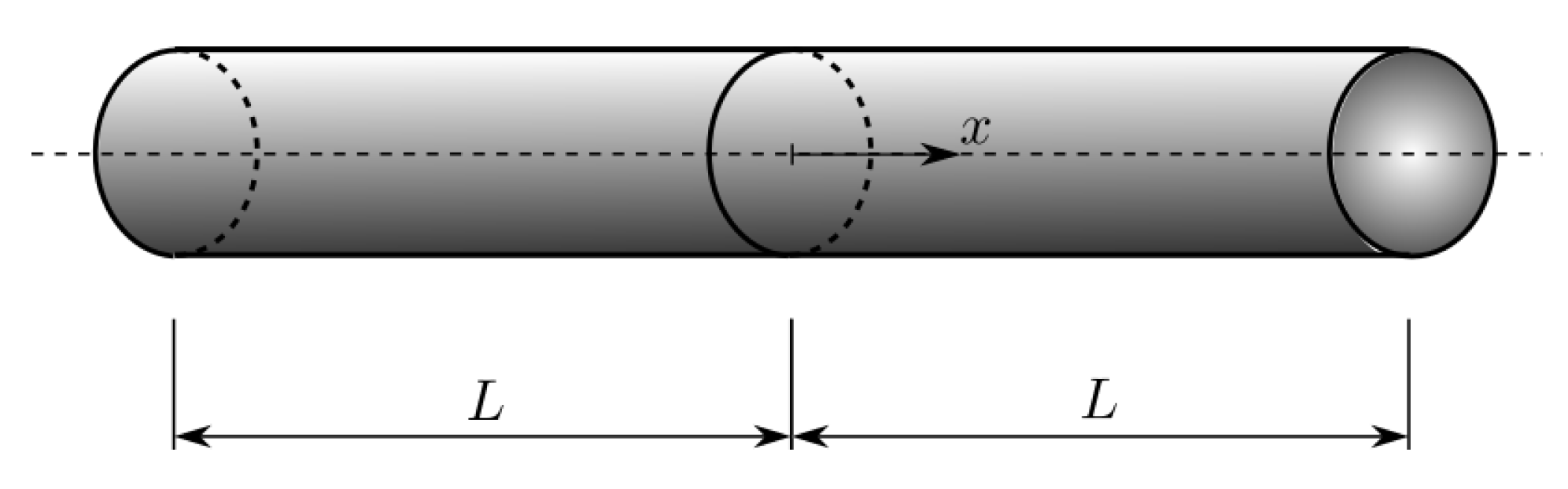
We consider a rod, defined as a one-dimensional (1D) solid, of length $2L$, as shown in Figure 1.

We assume that the relation between the stress $\sigma$ and the strain $ϵ$ in the rod may be expressed by [1,7]

$$\sigma (x)=E\left({\displaystyle {\beta }_1ϵ(x)+{\beta }_{2}k{\int }_{-L}^Lϵ(y)g(x-y)dy}\right),$$

(1)

where $x\in [-L,L]$, E is the Young’s modulus of the material, k is a positive constant typical of the material, g is the attenuation function and the strain $ϵ(x)$ can be derived from the longitudinal displacement $u(x)$ in the usual way through the compatibility equation

$$ϵ(x)=\frac{du}{dx}.$$

(2)

It is noteworthy that the second term on the right side of Equation (1) is the convolution of classical stress $Eϵ$ with g. The attenuation function g characterises the nonlocal contribution of the elasticity and it is assumed to be [31]

$$g(z)={\displaystyle \frac{1}{\Gamma (2-2s){\left|z\right|}^{2s-1}}},$$

(3)

where $\Gamma$ denotes the Gamma function. In order to produce an attenuation it must be

$$\frac{1}{2}<s<1.$$

(4)

The coefficients ${\beta }_1$ and ${\beta }_2$ have the physical meaning of denoting the importance of the local and the nonlocal behaviour, respectively, and they must obey to the following relations:

$${\beta }_1+{\beta }_2=1,{\beta }_1\in [0,1].$$

(5)

The balance equation is

$${\sigma }^{\prime }(x)+b(x)=0,$$

(6)

where $b(x)$ it the distributed load applied to the rod

The fractional Laplacian operator ${(-\Delta )}^s$ is defined for 1D case as

$${(-\Delta )}^s\phi (x)={\mathcal{F}}^{-1}\left({\left|\xi \right|}^{2s}\mathcal{F}(\phi (\xi ))\right)\forall x,\xi \in \mathbb{R},$$

(7)

where $\mathcal{F}$ and ${\mathcal{F}}^{-1}$ denote the direct and inverse Fourier transforms. The preceding is equivalent, for a function $\phi (x)$ with $x\in [-L,L]$ and $\frac{1}{2}<s<1$, to [27]

$${(-\Delta )}^s\phi (x)=\frac{{}_{-L}{D}_x^{2s}\phi (x)+{}_x{D}_L^{2s}\phi (x)}{2cos(s\pi )},$$

(8)

where ${}_{-L}{D}_x^{2s}\phi (x)$ and ${}_x{D}_L^{2s}\phi (x)$ are the forward and backwards Riemann–Liouville fractional derivatives of order 2s, defined as

$${}_{-L}{D}_x^{2s}\phi (x)=\frac{1}{\Gamma (2-2s)}\frac{d^2}{d{x}^2}{\int }_{-L}^x\frac{\phi (x)}{{(x-\xi )}^{2s-1}}d\xi ,{}_x{D}_L^{2s}\phi (x)=\frac{1}{\Gamma (2-2s)}\frac{d^2}{d{x}^2}{\int }_x^L\frac{\phi (x)}{{(\xi -x)}^{2s-1}}d\xi .$$

(9)

With the approach employed in [27], using balance and compatibility equations together with Equation (1) the following problem can be defined

$$\left\{\begin{array}{c}-c{u}^{″}+\kappa {(-\Delta )}^{s}u={\displaystyle \frac{b(x)}{E}}x\in [-L,L]\hfill \\ u(x)=u^{\prime }(x)=0x=\pm L,\hfill \end{array}\right.$$

(10)

where ${(-\Delta )}^s$ is the fractional Laplacian operator of order s, with $\frac{1}{2}<s<1$, $c={\beta }_1\in [0,1]$ and $\kappa =-2{\beta }_{2}kcoss\pi$ and ${\beta }_2=-{\beta }_1$. Note that since $k>0$ we have $\kappa \ge 0$.

2.2. The Local/Nonlocal Differential Model

A different approach to model the behaviour of the rod taking into account both the local and nonlocal effects has been proposed in [33], based on the model proposed in [1]. The relation between the stress and the strain is given by the following (please note that in this case $x\in [0,L]$)

$$\sigma (x)={\xi }_{1}Eϵ(x)+{\xi }_{2}E{\int }_0^L{\mathcal{K}}_l(x,y)ϵ(y)dy,$$

(11)

where ${\mathcal{K}}_l$ is a kernel function given by

$${\mathcal{K}}_l=\frac{1}{2l}{e}^{-{\displaystyle \frac{|x-y|}{l}}}$$

(12)

and $l>0$ is the characteristic length. It is worth noting that as $l>>L$ the rod can be considered subjected to self-tension. Since both local and nonlocal effects are considered, the (11) is denoted by the authors the local/nonlocal stress-strain law. Moreover, Equation (11), together with Equations (2) and (6), constitutes the strong form of the problem, which can be reduced to a weak form through test functions $\tilde{v}(z)$ with $\tilde{v}(-L)=\tilde{v}(L)=0$ [34].

It is noteworthy that, even if ${\xi }_1$ and ${\xi }_2$ are similar to ${\beta }_1$ and ${\beta }_2$ since they are related to the fraction of local and nonlocal behaviour, respectively, we maintained two different sets of symbols since their use is slightly dissimilar.

The differential equation to be solved is found using the balance and compatibility equations together with Equation (11) [33]

$$({\xi }_1+{\xi }_2)ϵ(x)-{\xi }_1{l}^2{ϵ}^{″}(x)=\frac{1}{E}\left(f(x)-l^2{f}^{″}(x)\right),$$

(13)

where

$$f(x)=-\int b(x)dx+C=\sigma (x)$$

(14)

with C a constant to be determined.

An important part in [33] is devoted to establishing the boundary conditions (b.c.), which assure the consistency of the formulation, and in particular it is found that they are

$${\phi }^{\prime }(0)-\frac{1}{l}\phi (0)=0,{\phi }^{\prime }(L)-\frac{1}{l}\phi (L)=0,$$

(15)

where

$$\phi (x)={\displaystyle \frac{f(x)}{E{\xi }_1}}-ϵ(x).$$

(16)

In the case of purely local models, i.e., with ${\xi }_1=1$, the b.c. expressed by Equation (15) are always satisfied. As observed by the authors, while considering the purely nonlocal problem, i.e., with ${\xi }_1=0$, the b.c. may not be satisfied (as, for example, in the case of constant stress), in the case of local/nonlocal behaviour, i.e., ${\xi }_1\ne 0$ and ${\xi }_2\ne 0$, the b.c. can be satisfied since they do not impose any particular condition on the stress field.

Moreover, there is an important observation in [33] that we quote from

“Nevertheless, for a meaningful comparison between a nonlocal elasticity model and experimental size effect data, two important conditions must be satisfied: (i) the classical continuum theory is recovered for vanishing nonlocal length, and (ii) the nonlocal system is stiffer than the local one.”

In order to obtain that the nonlocal response is stiffer than the purely local one, it must be

$${\xi }_1\ge 1,{\xi }_1+{\xi }_2=1.$$

(17)

It is noteworthy that in this case the value of ${\xi }_2$ is negative. Instead, in the fractional Laplacian model, the value of ${\beta }_1$ must be smaller than 1 and therefore ${\beta }_2$ is greater than 0.

2.3. Nonlocal Rod Dynamics by Means of Fractional Laplacian Model

The fractional Laplacian model for the nonlocal rod was extended to dynamics in [32]. In particular, the D’Alembert principle was used and therefore the equilibrium equation is

$${\sigma }^{\prime }+f=\rho \ddot{u},$$

(18)

where $\rho =\rho (x)$ is the mass density. Since now $\sigma$ and u depend both in space and in time, partial derivatives denoted ${}^{\prime }=\frac{\partial }{\partial x}$ and $\dot{}=\frac{\partial }{\partial t}$ are used. For simplicity, it is assumed that the mass density $\rho$ is a positive constant.

By using the approach in [32] the following problem can be defined

$$\left\{\begin{array}{c}-c{u}^{″}(x,t)+\kappa {(-\Delta )}^{s}u(x,t)+{\displaystyle \frac{1}{v^2}}\ddot{u}(x,t)={\displaystyle \frac{b(x,t)}{E}}x\in [-L,L],\forall t\hfill \\ u(x,t)=0x=\pm L,\forall t\hfill \\ u(x,0)=u_0(x)\hfill \\ \dot{u}(x,0)={\dot{u}}_0(x)\hfill \end{array}\right.,$$

(19)

where $v={\left(E/\rho \right)}^{1/2}$.

2.4. Numerical Approximation of Fractional Laplacian Problems

Both in the case of statics, see Equation (10), and dynamics, see Equation (19), there are difficulties in finding a closed-form solution. Therefore, a numerical approximation is sought. The main important item is the estimation of the fractional Laplacian, for which the approach introduced in [35] is used.

We look for the solution defined in a discrete number of points $x_i$ with $i=1,2,\dots ,n$

$$x_i=-L+ih,i=0,1,\dots ,n-1,$$

(20)

with $h=2L/(n-1)$. The values of displacement u at $x_i$ is denoted by $u_i$.

A central difference approximation is used for the second derivative $u^{″}$:

$$u_i^{″}={\displaystyle \frac{u_{i+1}-2u_i+u_{i-1}}{h^2}}.$$

(21)

When $i=0$ and $i=n-1$, the second-order forward and backwards approximation, respectively, are used to estimate the second derivative. Moreover, it is noteworthy that the central difference approximation used for the second derivative is coherent with classical dynamic models, for example, to express the wave equation of a series of masses connected by linear springs.

The fractional Laplacian operator ${(-\Delta )}^s$ is approximated as

$${(-{\Delta }_h)}^s{u}_i=\sum _{j=1}^{\infty }\left(2u_i-u_{i+j}-u_{i-j}\right)w_j=\sum _{j=-\infty }^{\infty }\left(u_i-u_{i-j}\right)w_j,$$

(22)

where $w_j$ are weights, determined by a semi-exact quadrature rule, given in [35]. The formula in Equation (22) is similar to the central difference approximation formula in Equation (21); anyway, the sum is extended to all the points with weights that decrease with the difference $|i-j|$. It is possible to prove that Equation (22) reduces to the finite differences approximation of Equation (21) as s approaches unity.

The fractional Laplacian is estimated considering only $M\ge n-1$ terms in Equation (22)

$${(-{\Delta }_h)}_M^s{u}_i=\sum _{j=-M}^M\left(u_i-u_{i-j}\right)w_j+\frac{C_{1,s}}{s{(Mh)}^{2s}}u(x_i),$$

(23)

and for $Mh\ge 2L$ the values of $C_{1,s}$ are given in [27]

$$C_{1,s}=s{2}^{2s}\frac{\Gamma (s+1/2)}{{\pi }^{1/2}\Gamma (1-s)}.$$

(24)

Therefore, the discrete form of Equation (10) is

$$\left\{\begin{array}{c}-c\left({\displaystyle \frac{u_{i+1}-2u_i+u_{i-1}}{h^2}}\right)+\kappa {(-{\Delta }_h)}_M^s{u}_i={\displaystyle \frac{b_i}{E}}\mathrm{for} i=1,2,\dots ,n-2\hfill \\ u_0=u_{n-1}=0\hfill \end{array}\right.$$

(25)

with $b_i=b(x_i)$. In the first equation, i is in the range $1\dots n-2$ since values 0 and $n-1$ are included in the second equation.

In dynamics, a discretisation of the problem in the time domain is also necessary. In particular m time steps equally spaced are used

$$t_j=j\Delta T,j=0,1,\dots ,m-1,$$

(26)

with $\Delta T=T/(m-1)$, T being the length of the time history.

To this aim the Newmark’s method is used [36], which allows estimating the velocity and displacement at the time $t_{j+1}$ as

$$\left\{\begin{array}{c}{}^{j+1}{\dot{u}}_i={}^j{\dot{u}}_i+\left[\left(1-\gamma \right)\Delta t\right]{}^j{\ddot{u}}_i+\left(\gamma \Delta t\right){}^{j+1}{\ddot{u}}_i\hfill \\ {}^{j+1}{u}_i={}^j{u}_i+(\Delta t){}^j{\dot{u}}_i+\left[\left(0.5-\beta \right){(\Delta t)}^2\right]{}^j{\ddot{u}}_i+\left[\beta {(\Delta t)}^2\right]{}^{j+1}{\ddot{u}}_i\hfill \end{array}\right.,$$

(27)

where ${}^j{u}_i=u(x_i,t_j)$, ${}^j{\dot{u}}_i=\dot{u}(x_i,t_j)$ and ${}^j{\ddot{u}}_i=\ddot{u}(x_i,t_j)$. Since the acceleration at time $t_{j+1}$ is not known, the Newmark’s method is implicit. With $\gamma =\frac{1}{2}$ and $\beta =\frac{1}{4}$ a constant average acceleration between $t_j$ and $t_{j+1}$ is assumed, while $\gamma =\frac{1}{2}$ and $\beta =\frac{1}{6}$ corresponds to assuming a linear variation of acceleration between $t_j$ and $t_{j+1}$. In order to ave numerical stability, $\gamma =1/2$ and $\beta =1/4$ have been used.

By means of Equation (27) the discrete form of (19) is

$$\left\{\begin{array}{c}-c{}^{j+1}\left({\displaystyle \frac{{}^{j+1}{u}_{i+1}-2{}^{j+1}{u}_i+{}^{j+1}{u}_{i-1}}{h^2}}\right)+\kappa {(-{\Delta }_h)}_M^s{}^{j+1}{u}_i+{\displaystyle \frac{1}{v^2}}{}^{j+1}\ddot{u_i}={\displaystyle \frac{{}^{j+1}{b}_i}{E}}\mathrm{for} i=1,2,\dots ,n-2\hfill \\ u_0(t)=u_{n-1}(t)=0\hfill \end{array}\right.$$

(28)

where ${}^{j+1}{b}_i=b(x_i,t_{j+1})$.

The problems to be solved are therefore: find the values of $u_i$ in statics and ${}^{j+1}{\ddot{u}}_i$ for each j in dynamics in order to find the zeros of the vectorial function g expressed by (25) and (28), respectively.

The problem has been solved numerically using the Python programming language and in particular its procedure “fsolve”, based on the Powell hybrid method, as implemented in MINPACK, see [37].

3. Results

3.1. The Local/Nonlocal Differential Model

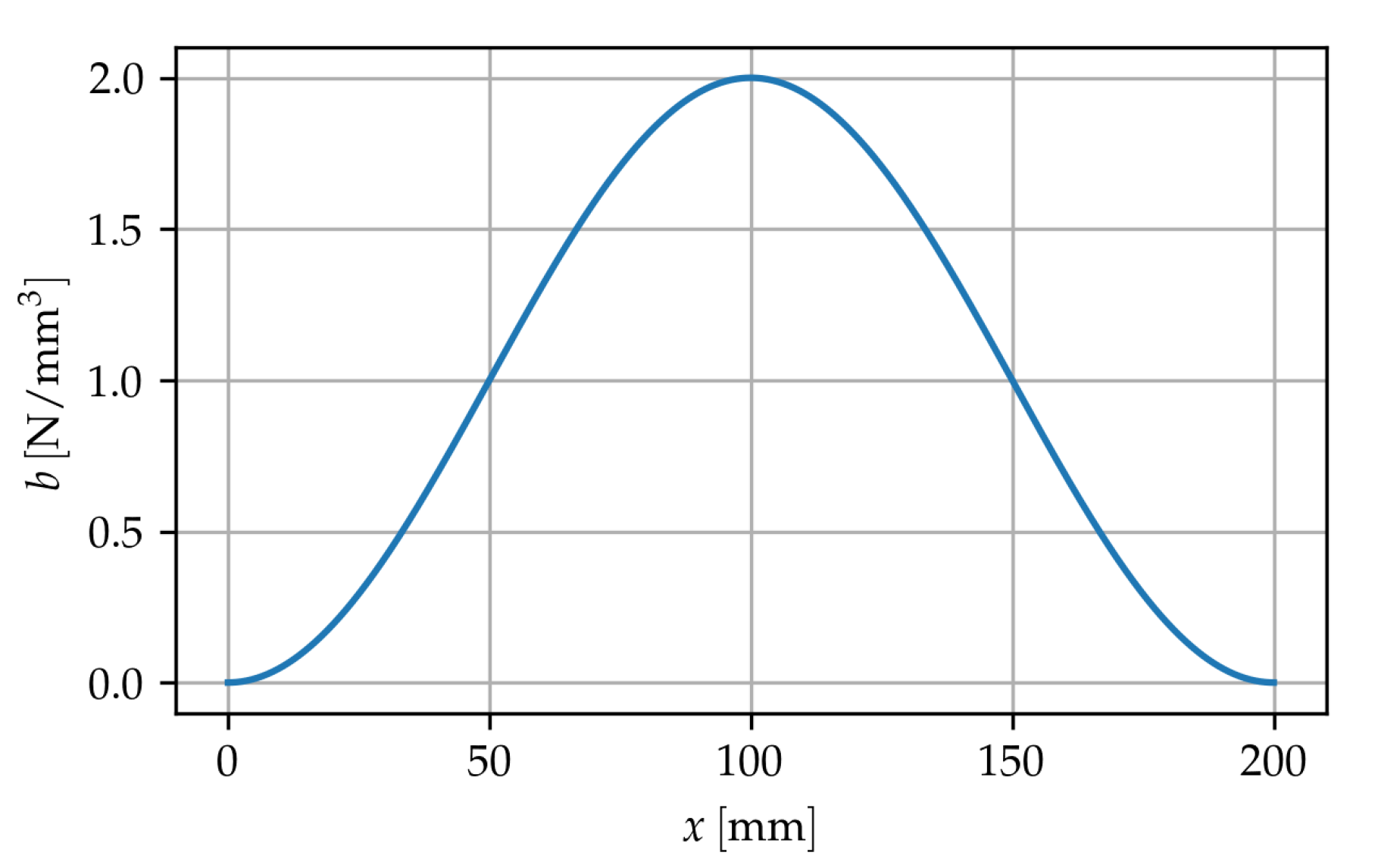
The model proposed by [33] has been applied to the case of the rod having both a local and nonlocal behaviour and subjected to a distributed load given by the following law

$$b(x)=1+cos\left(\frac{2\pi }{L}\left(x-\frac{L}{2}\right)\right)$$

(29)

where $0\le x\le L$. In this case, the stress field $f(x)$ is given by

$$f(x)=-\int b(x)dx+C=-x-\frac{L}{2\pi }sin\left(\frac{2\pi }{L}\left(x-\frac{L}{2}\right)\right)+C$$

(30)

and therefore

$$f^{″}(x)=\frac{2\pi }{L}sin\left(\frac{2\pi }{L}\left(x-\frac{L}{2}\right)\right).$$

(31)

The overall force acting on the rod is given by

$$B={\int }_0^{L}b(x)dx={\left|x+\frac{L}{2\pi }sin\left(\frac{2\pi }{L}\left(x-\frac{L}{2}\right)\right)\right|}_0^L=L$$

(32)

and, considering the symmetry of the problem, both in geometry and in the loading, the reaction at both ends is equal to $-L/2$.

The value of the stress on the left end allows to evaluate the value of C

$$\sigma (0)=f(0)=\frac{L}{2}\Rightarrow C=\frac{L}{2}$$

(33)

and, as expected, the stress at the right end is

$$\sigma (L)=f(L)=-\frac{L}{2}.$$

(34)

The solution is given by solving Equation (13) and it is

$$\begin{array}{c}\epsilon (x)=\frac{C}{E\left({\xi }_1+{\xi }_2\right)}+C_1{e}^{-\frac{x\sqrt{1+\frac{{\xi }_2}{{\xi }_1}}}{l}}+C_2{e}^{\frac{x\sqrt{1+\frac{{\xi }_2}{{\xi }_1}}}{l}}\hfill \\ \hfill +\frac{L^{3}sin\left(\frac{2\pi x}{L}\right)}{2\pi E\left(L^2{\xi }_1+L^2{\xi }_2+4{\pi }^2{\xi }_1{l}^2\right)}+\frac{2\pi L{l}^{2}sin\left(\frac{2\pi x}{L}\right)}{E\left(L^2{\xi }_1+L^2{\xi }_2+4{\pi }^2{\xi }_1{l}^2\right)}-\frac{x}{E\left({\xi }_1+{\xi }_2\right)}\end{array}$$

(35)

while to find the values of $C_1$ and $C_2$ the boundary conditions that assure the consistency of the formulation, given by Equation (15), must be applied. The expressions for $C_1$ and $C_2$ are rather cumbersome and are reported in Appendix A.

In the following the results for ${\xi }_1=1.4$ and $l=0.25L$, assuming $L=200\mathrm{mm}$ and $E=1000\mathrm{N}/\mathrm{mm}$, are reported.

The values of $b(x)$ are shown in Figure 2.

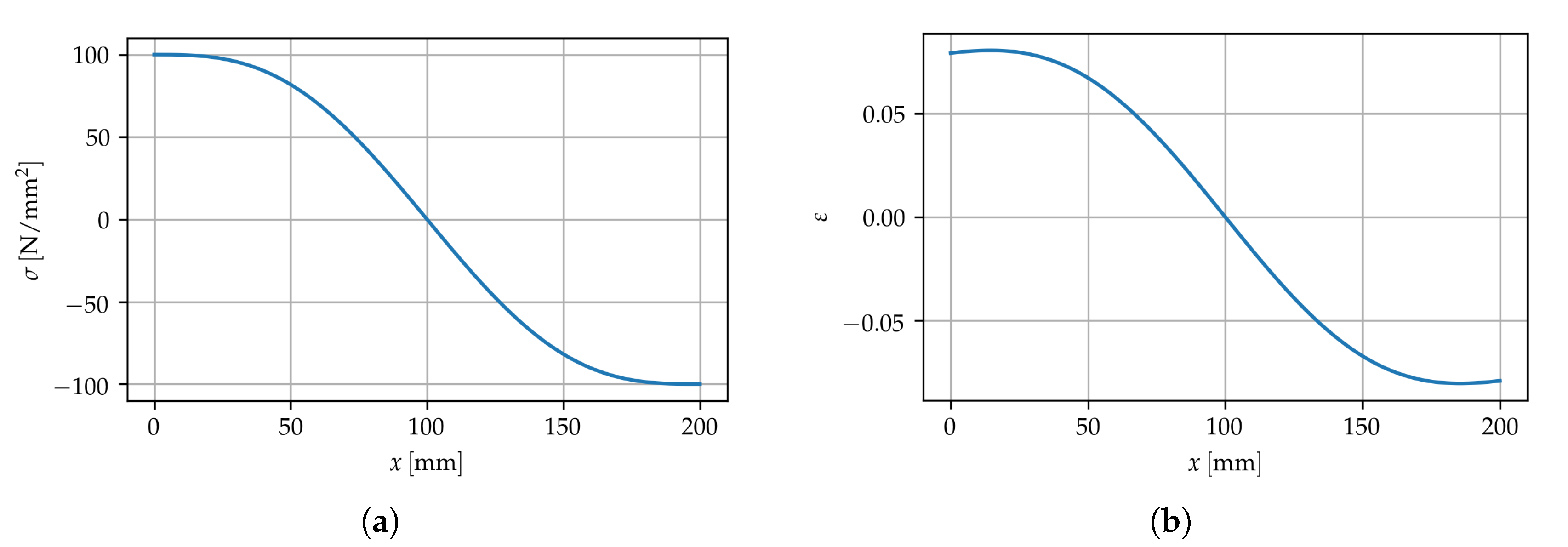
The values of stress $\sigma (x)$ and strain $\epsilon (x)$ are shown in Figure 3.

In order to compare the results with those obtained with the purely local theory, the strain is obtained from the balance Equation (6) and the relation between stress and strain given by the local law

$$ϵ(x)=\frac{\sigma (x)}{E}.$$

(36)

The derivative of the strain is

$${ϵ}^{\prime }(x)=\frac{{\sigma }^{\prime }(x)}{E}=\frac{1}{E}\left(-b(x)\right)$$

(37)

from which the value of $\epsilon$ can be found as

$$ϵ(x)=\frac{1}{E}\left(-\int b(x)dx+C\right)=\frac{1}{E}\left(f(x)\right).$$

(38)

The displacement at midspan is therefore

$$\begin{array}{c}u(L/2)=u(0)+{\int }_0^{L/2}ϵdx=u(0)+\frac{1}{E}{\int }_0^{L/2}fdx\hfill \\ \hspace{1em}\hspace{1em}\hspace{1em} =u(0)+\frac{1}{E}{\int }_0^{L/2}\left(-x-\frac{L}{2\pi }sin\left(\frac{2\pi }{L}\left(x-\frac{L}{2}\right)\right)+C\right)dx\hfill \\ \hspace{1em}\hspace{1em}\hspace{1em} =u(0)+\frac{1}{E}{\left|Cx-\frac{x^2}{2}+\frac{L^2}{{(2\pi )}^2}cos\left(\frac{2\pi }{L}\left(x-\frac{L}{2}\right)\right)\right|}_0^{L/2}=u(0)+\frac{1}{E}\left[C\frac{L}{2}-\frac{{(L/2)}^2}{2}+2\frac{L^2}{{(2\pi )}^2}\right].\hfill \end{array}$$

(39)

For comparison, since the displacement in the local/nonlocal case has not been estimated, the difference of displacement between the midspan and the left end is used:

$$\Delta u^{loc}=u(L/2)-u(0)=\frac{1}{E}\left[C\frac{L}{2}-\frac{{(L/2)}^2}{2}+2\frac{L^2}{{(2\pi )}^2}\right].$$

(40)

In the case of local/nonlocal behaviour, the difference is given by

$$\Delta u^{loc/noloc}={\int }_0^{L/2}\epsilon (x)dx,$$

(41)

where $\epsilon (x)$ is given by (35).

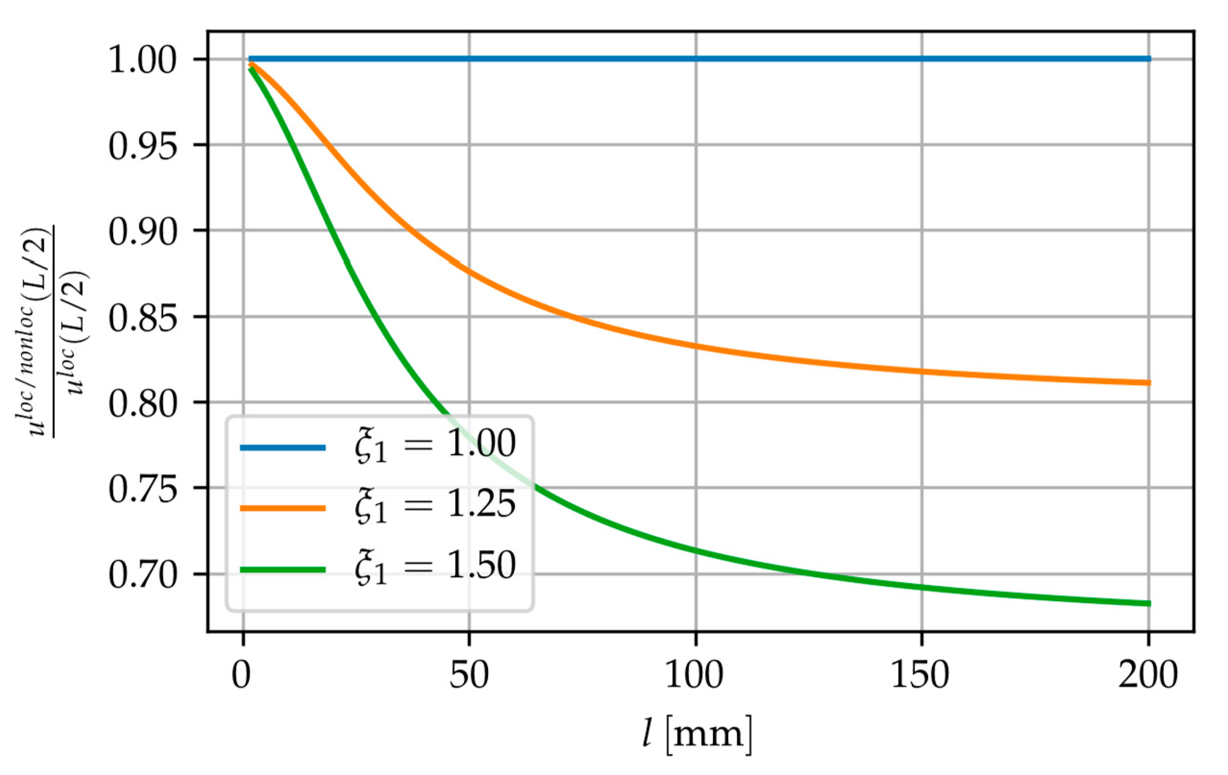
The comparison of midspan displacements between local and local/nonlocal behaviour for various values of ${\beta }_1$ and l are shown in Figure 4.

Since the solution of the local/nonlocal model is given in closed-form by Equation (35), we observe that there are not any singularities or critical point, and therefore the model is robust in order to estimate the behaviour of the rod under the given load. As can be appreciated, as l increases the local/nonlocal midspan displacement decreases, as expected. Moreover, as the response is more influenced by the nonlocal component, i.e., as the value of ${\xi }_1$ increases, the ratio $u^{local/nonlocal}/u^{local}$ decreases.

3.2. Fractional Laplacian Model and Comparison

The response of the rod under the same load is also evaluated by means of the fractional Laplacian approach, as recalled in Section 2.4. Nevertheless, since in the fractional Laplacian model $-L\le x\le L$ the applied load is

$$b(x)=1+cos\left(\frac{2\pi }{L}x\right).$$

(42)

The same value of $E=1000\mathrm{N}/{\mathrm{mm}}^2$ has been used. Moreover, $n=105$ and $M=105$.

In particular, the midspan displacement has been evaluated for several values of k and s, using different values of ${\beta }_1$. It is noteworthy that in the approach based on the fractional Laplacian the value of ${\beta }_1$ is always smaller or equal to 1, and therefore the value of ${\beta }_2$ is always greater or equal to zero, while in the approach of [33] the value of ${\xi }_1$ (which has the same meaning of ${\beta }_1$) must be greater or equal 1 and therefore ${\xi }_2$ (which has the same meaning of ${\beta }_2$) is smaller or equal 0.

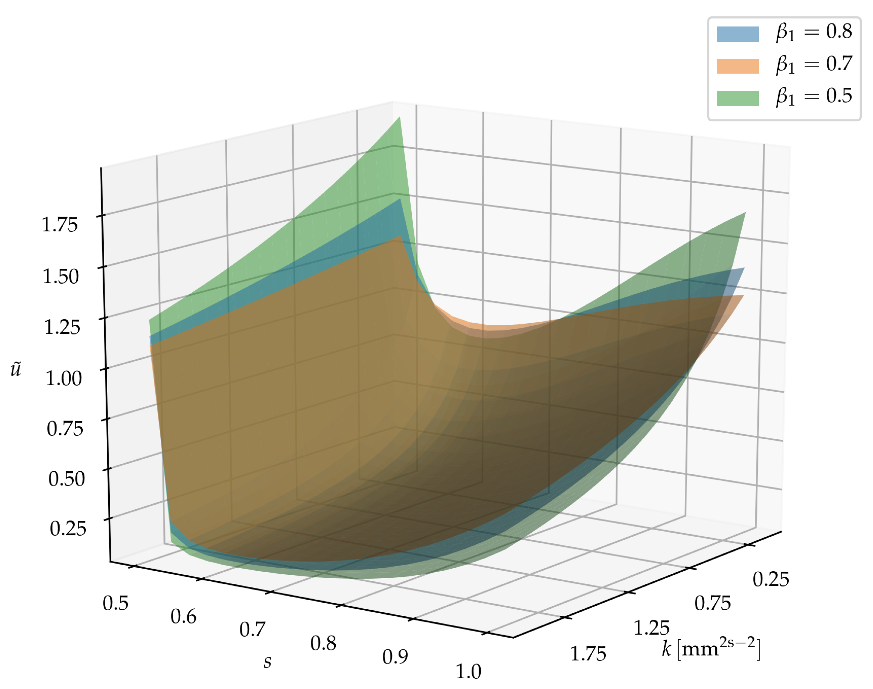
In order to present the results, the surface of the ratio of the midspan displacement for an assigned value of ${\beta }_1$ between the fractional model case and the local case is considered to be a function of k and s as follows

$$\tilde{u}({\beta }_1,k,s)=\frac{u^{frac.Lap.}(L/2)}{u^{local}(L/2)}.$$

(43)

In Figure 5, the results for three different values of ${\beta }_1$: 0.5, 0.7, 0.8 are shown.

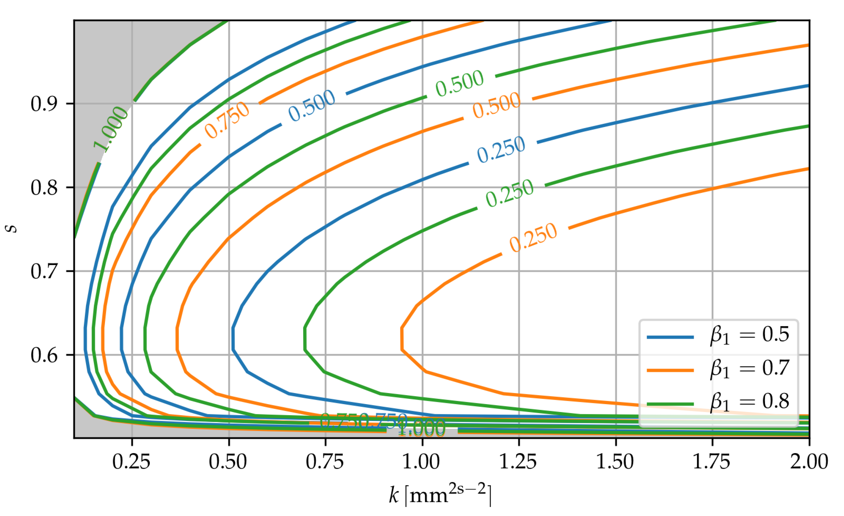
The results are reported in Figure 6 in terms of level curves.

It is noteworthy that the same ratio for a fixed ${\beta }_1$ can be obtained with two different sets of values of k and s: for each of the set a different deformed shape is obtained.

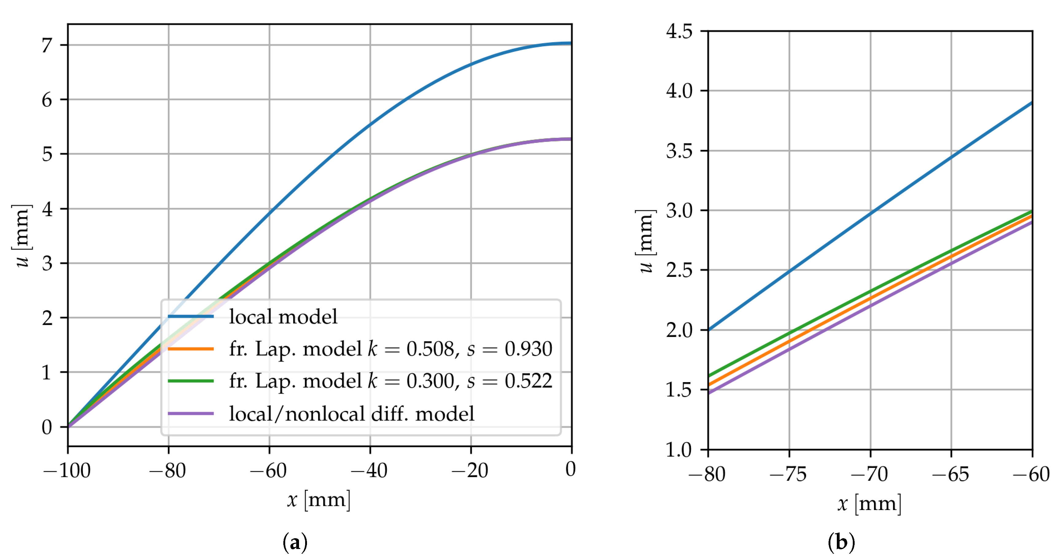
As an example, in Figure 7 we compare the displacements obtained with the local/nonlocal differential model with a value of $l=65\mathrm{mm}$ and ${\xi }_1=1.5$ and the displacements obtained with the fractional Laplacian model using $k=0.508{\mathrm{mm}}^{2\mathrm{s}-2}$ and $s=0.930$ in one case and $k=0.300{\mathrm{mm}}^{2\mathrm{s}-2}$ and $s=0.522$ in the other case; in both cases, ${\beta }_1=0.5$. In all cases, the ratio of the nonlocal displacement and the local displacement at midspan is equal to 0.75.

As can be appreciated, the deformed shape is slightly different, and moreover the local/nonlocal differential model seems to give slightly smaller values of displacements between the rod end and midspan; anyway, in this case, the mean relative difference, defined as

$$\frac{1}{200}{\int }_{-100}^{100}\frac{u^{frac.Lap.}(x)-u^{local}(x)}{u^{local}(x)}dx$$

(44)

where $u^{frac.Lap.}(x)$ are the displacements obtained with the fractional Laplacian model and $u^{local}(x)$ are the displacements obtained with local/nonlocal differential model, is below 5%.

3.3. Response in Dynamics

The rod is considered to be subjected to a distributed load given by

$$b(x,t)=\left(sin\left(\frac{2\pi }{T_0}t\right)\right)\left(1+cos\left(\frac{2\pi }{2L}x\right)\right).$$

(45)

We recall from [27] that in the local case the value of the first natural period is $T_1=2L/v$ and therefore assuming $\rho =1\mathrm{kg}/{\mathrm{mm}}^3$ it is $T_1=12.65\mathrm{s}$. Moreover, the period of the nonlocal rod is always smaller than the local one.

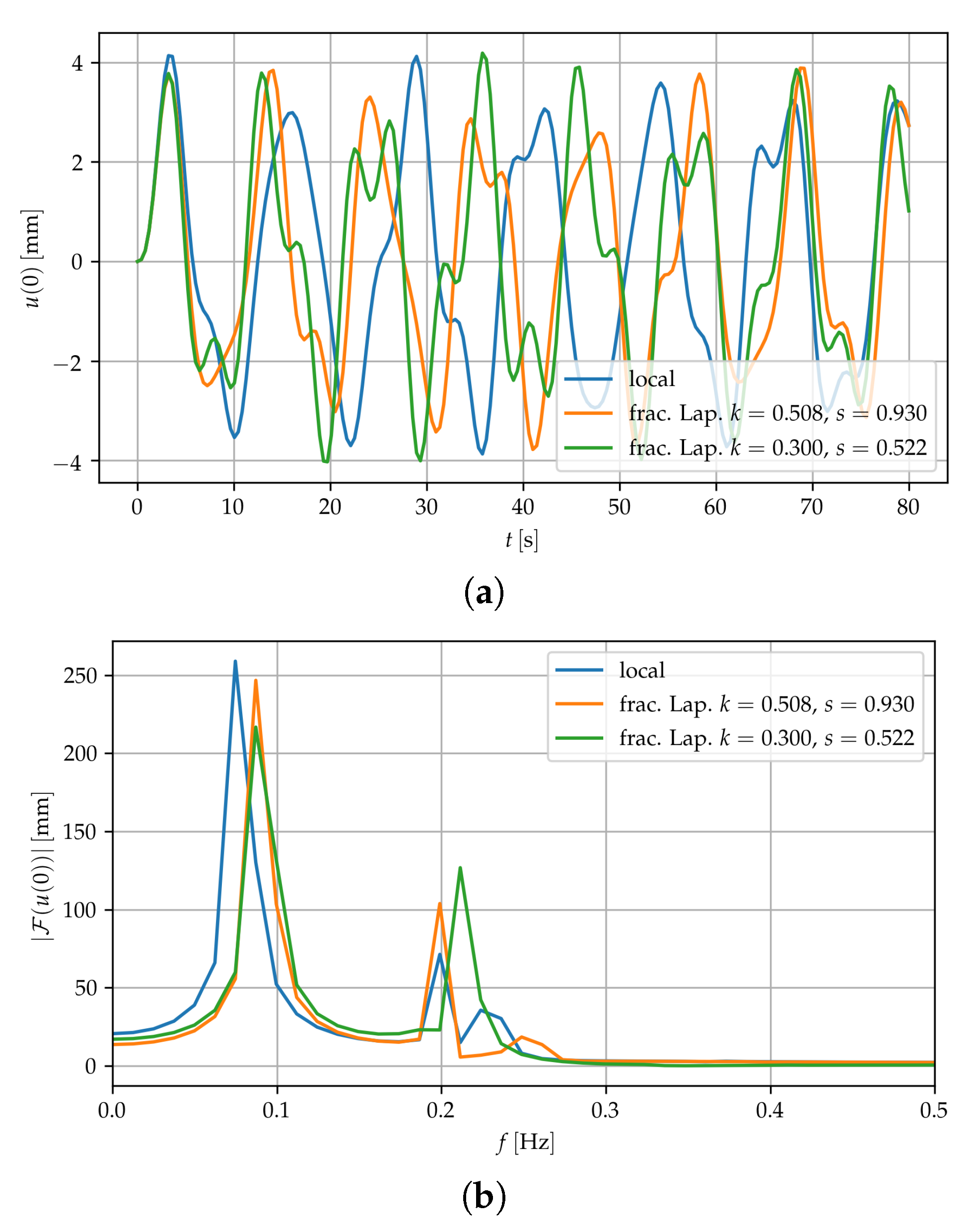
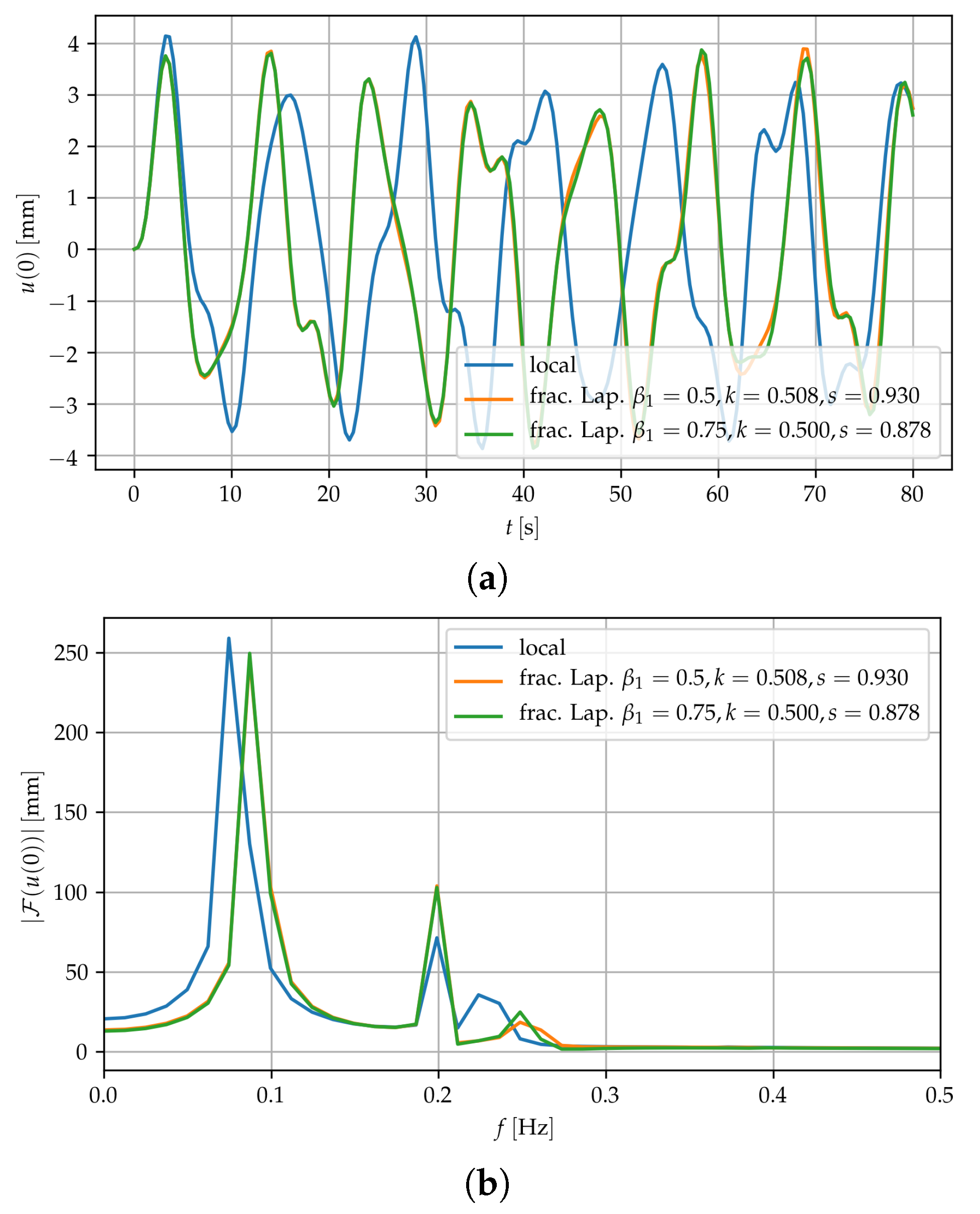
The period of the forcing function is assumed to be $T_0=5\mathrm{s}$ and the duration of the time history is $T=80\mathrm{s}$. The results are shown in Figure 8 both in the time domain and in the frequency domain (through the magnitude of the discrete Fourier transform values) in terms of midspan displacement for the local case and the nonlocal case, using the fractional Laplacian model with ${\beta }_1=0.5$ and the two different sets of values for k and s already used in the previous section.

From the figure we can appreciate that the nonlocal case is stiffer since the period decreases, as indicated by the intersections with the time axis and more clearly by the peak values in the frequency domain. Moreover, the difference in terms of displacement is also affected by the dynamical amplification factor, since the ratio between the forcing frequency and the natural frequency decreases.

Moreover, in Figure 9 the effect of different values of ${\beta }_1$ is shown. For ${\beta }_1=0.75$ we calibrated the values of k and s to give the same ratio of midspan displacement than ${\beta }_1=0.5$.

In this case, the difference is much smaller between the two nonlocal cases, since the chosen parameters determine the same ratio of midspan displacement and moreover the values of k and s are very similar, so the deformation is almost the same.

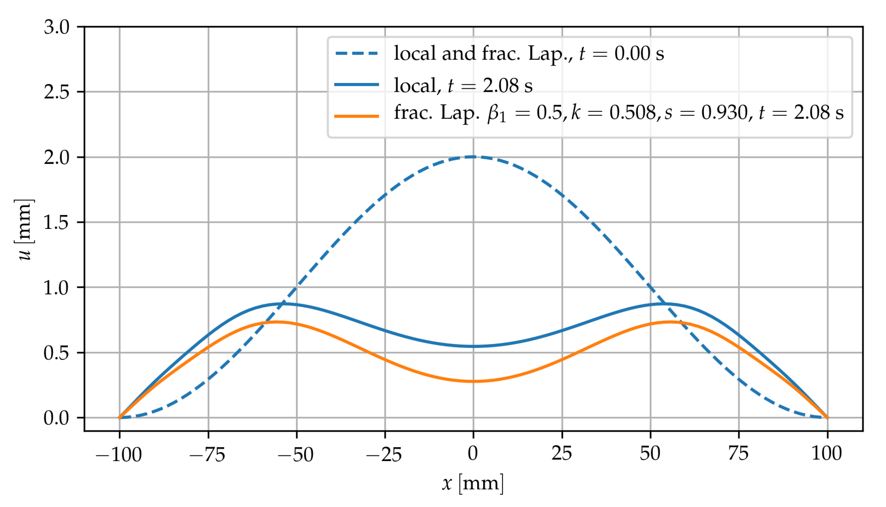
Moreover, the dynamics in the case of an unloaded rod with an assigned initial shape and zero initial velocity has been analysed. Assuming an initial shape given by

$$u(x,0)=1+cos\left(\frac{2\pi }{2L}x\right)$$

(46)

we obtain the results shown in Figure 10 with the same parameters of the nonlocal rod considered before. The results for the local case can also be obtained by means of superposition of classical wave solutions to 1D Navier’s equation.

Since the local/nonlocal is stiffer, after an equal amount of time its deformed shape is closer to the rest position, as expected.

4. Discussion and Conclusions

In the present paper, an approach to analyse the dynamics of a rod with a nonlocal elastic behaviour is proposed. This is based on the fractional Laplacian model, and requires the estimation of two parameters, k and s, where s is the order of the fractional Laplacian. Even if alternative approaches exist, for example, the local/nonlocal differential one [33], which is based on Eringen’s theory [7] and require only one parameter l, the present model can be useful in calibrating the estimated response more adequately to experimental results, for example, to accommodate both the midspan displacement and the mean displacement gradient of the rod. Moreover, the fractional Laplacian model requires that both the parameters weighting the local and nonlocal relative behaviour, ${\beta }_1$ and ${\beta }_2$, are positive, while in the local/nonlocal differential one the corresponding parameter, ${\xi }_1$ and ${\xi }_2$, are positive and negative, respectively, in order to reproduce experimental results. Nevertheless, the local/nonlocal differential model can be solved in closed-form for simple cases, while the fractional Laplacian one must resort to numerical methods in all cases. Moreover, it can be extended in dynamics in a rather straightforward way, and the solution can be approximated quite affordably by means of the time domain discretisation techniques: in the present paper, we propose to use Newmark’s method. This approach is very fast and appears to be suitable for analysing the rod under arbitrary excitations. The proposed fractional Laplacian model could also be used to model the bending of beams, plates, and in the same way it can be certainly extended to analyse waves in nonlocal elastic 3D solids; these are the topics of the ongoing research.

References

- Eringen, A.C.; Edelen, D.G.B. On nonlocal elasticity. Int. J. Eng. Sci. 1972, 10, 233–248. [Google Scholar] [CrossRef]
- Bazant, Z.P. Why continuum damage is nonlocal: Micromechanics argument. J. Eng. Mech. 1991, 117, 1070–1087. [Google Scholar] [CrossRef] [Green Version]
- Atanackovic, T.M.; Stankovic, B. Generalized wave equation in nonlocal elasticity. Acta Mech. 2009, 208, 1–10. [Google Scholar] [CrossRef]
- Silling, S.A. Origin and Effect of Nonlocality in a Composite—Sandia Report SAND2013-8140; Sandia National Laboratories: Albuquerque, NM, USA, 2014. [Google Scholar]
- Challamel, N. Static and dynamic behaviour of nonlocal elastic bar using integral strain-based and peridynamic models. C. R. Mech. 2018, 346, 320–335. [Google Scholar] [CrossRef]
- Eringen, A.C. Nonlocal Continuum Field Theories; Springer: New York, NY, USA, 2002. [Google Scholar]
- Eringen, A.C. Vistas of nonlocal continuum physics. Int. J. Eng. Sci. 1992, 30, 1551–1565. [Google Scholar] [CrossRef]
- Barretta, R.; Feo, L.; Luciano, R.; Marotti de Sciarra, F. Application of an enhanced version of the Eringen differential model to nanotechnology. Compos. Part B Eng. 2016, 96, 274–280. [Google Scholar] [CrossRef]
- Romano, G.; Barretta, R. Stress-driven versus strain-driven nonlocal integral model for elastic nano-beams. Compos. Part B Eng. 2017, 114, 184–188. [Google Scholar] [CrossRef]
- Silling, S.A.; Zimmermann, M.; Abeyaratne, R. Deformation of a peridynamic bar. J. Elast. 2003, 73, 173–190. [Google Scholar] [CrossRef]
- Apuzzo, A.; Barretta, R.; Canadija, M.; Feo, L.; Luciano, R.; Marotti de Sciarra, F. A closed-form model for torsion of nanobeams with an enhanced nonlocal formulation. Compos. Part B Eng. 2017, 108, 315–324. [Google Scholar] [CrossRef]
- Fakher, M.; Rahmanian, S.; Hosseini-Hashemi, S. On the carbon nanotube mass nanosensor by integral form of nonlocal elasticity. Int. J. Mech. Sci. 2019, 150, 445–457. [Google Scholar] [CrossRef]
- De Rosa, M.A.; Lippiello, M. Nonlocal Timoshenko frequency analysis of single-walled carbon nanotube with attached mass: An alternative hamiltonian approach. Compos. Part B Eng. 2017, 111, 409–418. [Google Scholar] [CrossRef]
- Shen, Z.-B.; Sheng, L.-P.; Li, X.-F.; Tang, G.-J. Nonlocal Timoshenko beam theory for vibration of carbon nanotube-based biosensor. Physica E 2002, 44, 1169–1175. [Google Scholar] [CrossRef]
- Barretta, R.; Ali Faghidian, S.; de Sciarra, F.M.; Pinnola, F.P. Timoshenko nonlocal strain gradient nanobeams: Variational consistency, exact solutions and carbon nanotube Young moduli. Mech. Adv. Mater. Struct. 2019. [Google Scholar] [CrossRef]
- Liaskos, K.N.; Pantelous, A.A.; Kougioumtzoglou, I.A.; Meimaris, A.T.; Pirrotta, A. Implicit analytic solutions for a nonlinear fractional partial differential beam equation. Commun. Nonlinear Sci. Numer. Simul. 2020, 85, 105219. [Google Scholar] [CrossRef]
- Alotta, G.; Failla, G.; Pinnola, F.P. Stochastic analysis of a nonlocal fractional viscoelastic bar forced by Gaussian white noise. ASCE-ASME J. Risk. Uncertain. Eng. Syst. Part B Mech. Eng. 2017, 3, 030904. [Google Scholar] [CrossRef]
- Alotta, G.; Di Paola, M.; Failla, G.; Pinnola, F.P. On the dynamics of non-local fractional viscoelastic beams under stochastic agencies. Compos. Part B Eng. 2018, 137, 102–110. [Google Scholar] [CrossRef]
- Śniady, P.; Podwórna, M.; Idzikowski, R. Stochastic vibrations of the Euler–Bernoulli beam based on various versions of the gradient nonlocal elasticity theory. Probab. Eng. Mech. 2019, 56, 27–34. [Google Scholar] [CrossRef]
- Fuschi, P.; Pisano, A.A.; De Domenico, D. Plane stress problems in nonlocal elasticity: Finite element solutions with a strain-difference-based formulation. J. Math. Anal. Appl. 2015, 431, 714–736. [Google Scholar] [CrossRef]
- Tuna, M.; Kirca, M.; Trovalusci, P. Deformation of atomic models and their equivalent continuum counterparts using Eringen’s two-phase local/nonlocal model. Mech. Res. Commun. 2019, 97, 26–32. [Google Scholar] [CrossRef] [Green Version]
- Pinnola, F.P.; Ali Faghidian, S.; Barretta, R.; Marotti de Sciarra, F. Variationally consistent dynamics of nonlocal gradient elastic beams. Int. J. Eng. Sci. 2020, 149, 103220. [Google Scholar] [CrossRef]
- Romano, G.; Barretta, R.; Diaco, M.; Marotti de Sciarra, F. Constitutive boundary conditions and paradoxes in nonlocal elastic nanobeams. Int. J. Mech. Sci. 2017, 121, 151–156. [Google Scholar] [CrossRef]
- Li, G.; Xing, Y.; Wang, Z.; Sun, Q. Effect of boundary conditions and constitutive relations on the free vibration of nonlocal beams. Results Phys. 2020, 19, 103414. [Google Scholar] [CrossRef]
- Carpinteri, A.; Cornetti, P.; Sapora, A. Static-kinematic fractional operators for fractal and nonlocal solids. Z. Angew. Math. Mech. 2009, 89, 207–217. [Google Scholar] [CrossRef]
- Di Paola, M.; Zingales, M. Long-range cohesive interactions of nonlocal continuum faced by fractional calculus. Int. J. Solids Struct. 2008, 45, 5642–5659. [Google Scholar] [CrossRef] [Green Version]
- Autori, G.; Cluni, F.; Gusella, V.; Pucci, P. Mathematical models for nonlocal elastic composite materials. Adv. Nonlinear Anal. 2017, 6, 355–382. [Google Scholar] [CrossRef]
- Autuori, G.; Cluni, F.; Gusella, V.; Pucci, P. Effects of the fractional laplacian order on the nonlocal elastic rod response. ASCE-ASME J. Risk. Uncertain. Eng. Syst. Part B Mech. Eng. 2017, 3, 030902. [Google Scholar] [CrossRef]
- Tarasov, V.E. Fractional gradient elasticity from spatial dispersion law. Condens. Matter Phys. 2014, 2014, 794097. [Google Scholar] [CrossRef] [Green Version]
- Cottone, G.; Di Paola, M.; Zingales, M. Elastic waves propagation in 1D fractional nonlocal continuum. Physica E 2009, 42, 95–103. [Google Scholar] [CrossRef]
- Sapora, A.; Cornetti, P.; Carpinteri, A. Wave propagation in nonlocal elastic continua modelled by a fractional calculus approach. Commun. Nonlinear Sci. Numer. Simul. 2013, 18, 63–74. [Google Scholar] [CrossRef]
- Autuori, G.; Cluni, F.; Gusella, V.; Pucci, P. Longitudinal waves in a nonlocal rod by fractional Laplacian. Mech. Adv. Mater. Struct. 2020, 27, 599–604. [Google Scholar] [CrossRef]
- Benvenuti, E.; Simone, A. One-dimensional nonlocal and gradient elasticity: Closed-form solution and size effect. Mech. Res. Commun. 2013, 48, 46–51. [Google Scholar] [CrossRef]
- Evragov, A.; Bellido, J.C. From non-local Eringen’s model to fractional elasticity. Mech. Res. Commun. 2019, 24, 1935–1953. [Google Scholar]
- Huang, Y.; Oberman, A. Numerical methods for the fractional Laplacian: A finite difference-quadrature approach. SIAM J. Numer. Anal. 2014, 52, 3056–3084. [Google Scholar] [CrossRef]
- Chopra, A.K. Dynamics of Structures; Pearson Prentice Hall: Upper Saddle River, NJ, USA, 2007. [Google Scholar]
- Moré, J.J.; Garbow, B.S.; Hillstrom, K.E. User Guide for MINPACK-1—Technical Report ANL-80-74; Argonne National Laboratory: Lemont, IL, USA, 1980.
- Meurer, A.; Smith, C.P.; Paprocki, M.; Čertík, O.; Kirpichev, S.B.; Rocklin, M.; Kumar, A.; Ivanov, S.; Moore, J.K.; Singh, S.; et al. SymPy: Symbolic computing in Python. PeerJ Comput. Sci. 2017, 3, e103. [Google Scholar] [CrossRef] [Green Version]
Figure 1.
Sketch of the rod with the reference axis.
Figure 2.
Values of for
Figure 3.
Respone of the rod to load : (a) stress , (b) strain .
Figure 4.
Ratio for different values of l and .
Figure 5.
Values of .
Figure 6.
Contour levels for the values of for different combinations of , k and s.
Figure 7.
Response of the rod to load : (a) displacements. (b) detailed view for . Parameters for local/nonlocal differential model: and . Parameters for fractional Laplacian model: , k and s shown in legend.
Figure 8.
Dynamic displacement in (a) time and (b) frequency domain for local case and the local/nonlocal case with and two different combination of k and s, which gives the same midspan displacement ratio: and ; and .
Figure 9.
Dynamic displacement in (a,b) time and (b) frequency domain local case and the local/nonlocal case with two combinations of , k and s, which gives the same midspan displacement ratio: , and ; , and .
Figure 10.
Displacements in dynamics for local case and the local/nonlocal case with , and at time instants and .
Publisher’s Note: MDPI stays neutral with regard to jurisdictional claims in published maps and institutional affiliations. |
© 2020 by the authors. Licensee MDPI, Basel, Switzerland. This article is an open access article distributed under the terms and conditions of the Creative Commons Attribution (CC BY) license (http://creativecommons.org/licenses/by/4.0/).
Share and Cite
MDPI and ACS Style
Gusella, V.; Autuori, G.; Pucci, P.; Cluni, F. Dynamics of Nonlocal Rod by Means of Fractional Laplacian. Symmetry 2020, 12, 1933. https://0-doi-org.brum.beds.ac.uk/10.3390/sym12121933
AMA Style
Gusella V, Autuori G, Pucci P, Cluni F. Dynamics of Nonlocal Rod by Means of Fractional Laplacian. Symmetry. 2020; 12(12):1933. https://0-doi-org.brum.beds.ac.uk/10.3390/sym12121933
Chicago/Turabian StyleGusella, Vittorio, Giuseppina Autuori, Patrizia Pucci, and Federico Cluni. 2020. "Dynamics of Nonlocal Rod by Means of Fractional Laplacian" Symmetry 12, no. 12: 1933. https://0-doi-org.brum.beds.ac.uk/10.3390/sym12121933
Note that from the first issue of 2016, this journal uses article numbers instead of page numbers. See further details here.