Generalized Attracting Horseshoe in the Rössler Attractor


1
Department of Computer Science, University of Illinois at Urbana-Champaign, Champaign, IL 61801, USA
2
Department of Applied Mathematics and Statistics, Stony Brook University, Stony Brook, NY 11794, USA
3
Department of Electrical and Computer Engineering, New Jersey Institute of Technology, Newark, NJ 07102, USA
4
Department of Applied Mathematics, University of Washington, Seattle, WA 98195, USA
5
Department of Mathematical Sciences, New Jersey Institute of Technology, Newark, NJ 07102, USA
*
Author to whom correspondence should be addressed.
Symmetry 2021, 13(1), 30; https://0-doi-org.brum.beds.ac.uk/10.3390/sym13010030
Submission received: 8 December 2020
/
Revised: 21 December 2020
/
Accepted: 21 December 2020
/
Published: 27 December 2020
(This article belongs to the Special Issue Symmetry in Modeling and Analysis of Dynamic Systems)
Abstract
:We show that there is a mildly nonlinear three-dimensional system of ordinary differential equations—realizable by a rather simple electronic circuit—capable of producing a generalized attracting horseshoe map. A system specifically designed to have a Poincaré section yielding the desired map is described, but not pursued due to its complexity, which makes the construction of a circuit realization exceedingly difficult. Instead, the generalized attracting horseshoe and its trapping region is obtained by using a carefully chosen Poincaré map of the Rössler attractor. Novel numerical techniques are employed to iterate the map of the trapping region to approximate the chaotic strange attractor contained in the generalized attracting horseshoe, and an electronic circuit is constructed to produce the map. Several potential applications of the idea of a generalized attracting horseshoe and a physical electronic circuit realization are proposed.
1. Introduction
The seminal work of Smale [1] showed that the existence of a horseshoe structure in the iterate space of a diffeomorphism is enough to prove it is chaotic. Often these diffeomorphisms arise from certain Poincaré maps of continuous-time chaotic strange attractors (CSA), which in turn are discrete-time CSAs. Some examples of such attractors are the Lorenz strange attractor [2], the Rössler attractor [3], and the double scroll attractor [4]. An example of a Poincaré map of the Lorenz equations is the Hénon map [5], which can be further simplified to the Lozi map [6]. Unsurprisingly, symmetry (and symmetry breaking) plays an important role in the analysis of these models.
In more recent years Joshi and Blackmore [7] developed an attracting horseshoe (AH) model for CSAs, which has two saddles and a sink. This, however, negates the possibility of the Hénon and Lozi maps, which have two saddles. Fortunately, the attracting horseshoe can be modified into a generalized attracting horseshoe (GAH), which can have either one or two saddles while still being an attracting horseshoe [8]. This results in a quadrilateral trapping region. While extensive analysis was done in Joshi et al. [8], a simple concrete example seemed to be illusive.
In this investigation, we implement novel numerical techniques to find the necessary Poincaré map of the Rössler attractor that would admit a quadrilateral trapping region. This trapping region represents a region of rotational symmetry as every iterate originating in the trapping region will return after a rotation. The trapping region would also filter out any flow that does not obey this symmetry. An electronic circuit could use these properties to isolate signals of interest. Similar to the experiments of Rahman et al. [9], we design a physical realization of the dynamical system in the form of an electronic circuit.
The remainder of the paper is organized as follows. In Section 2, we give an overview of the algorithm with the MATLAB codes included in the Supplementary Materials. Once we have the tools for our numerical experiments, we first propose a carefully constructed GAH model in Section 3. Then, we give numerical examples of Poincaré maps of the Rössler attractor and the map of interest in Section 4 and real-world examples in Section 5. Finally, we end discussions in Section 6 with some concluding remarks.
2. Poincaré Map Algorithm
To produce a general Poincaré section of a flow, we break up the program into four parts: solving the ODE; computing a Poincaré section perpendicular to either , , or ; rotating the Poincaré section; and iterating the Poincaré map. Solving the ODE is standard through ODE45 on MATLAB, which executes a modified Runge–Kutta scheme. Once we have our solution matrix, we need to approximate the values of first return maps from the discretized flow. By restricting the first return onto a Poincaré section, the iterate space of the Poincaré map can be visualized. This is easily done for a section perpendicular to the axes, but in order to locate a highly specialized object, such as the GAH, we need to be able to rotate the section. Once the desired section is found we can experiment on iterating the points of trapping region candidates.
The initial major task is approximating the first return map on a Poincaré section of a flow. Much of the ideas of our initial first return map code came from that of Gonze [10]. Once the discretized flow is found numerically a planar section for a certain value of x, y, or z can be defined, which in general will lie between pairs of simultaneous points. Then we may draw a line between the pair through the planar section and identify the intersecting point, which approximates a point of the first return map. This can also be done with more simultaneous points in order to get higher order approximations.
Once we can approximate a map for a section perpendicular to the axes we need to have the ability to rotate and move the map to any position. This is where our program completely diverges from that in [10]. While the first instinct might be to try to rotate the section, it is equivalent to rotate the flow in the opposite direction to the desired rotation of the section. Once the flow is rotated, the code for the first return map can be readily used. This gives us the ability to analyze the first return map of a general Poincaré section.
Finally, we would like to not only compute a first return map, but also compute the iterates of a Poincaré map of any system; that is, given an initial condition on an arbitrary Poincaré section can we find the subsequent iterates. To accomplish this, we solve the ODE for a given initial condition on the planar section to find the first return. Once we have the first return, we record its location and use that as the new initial condition. This iterates the map for as many returns as desired, thereby filling in a Poincaré map. Now we have the tools needed to run numerical experiments on GAHs.
3. A Constructed GAH System
In this section, we give a brief description of the generalized attracting horseshoe (GAH) map and devise a three-dimensional nonlinear ordinary differential equation with a Poincaré section that produces it.
3.1. The GAH Map
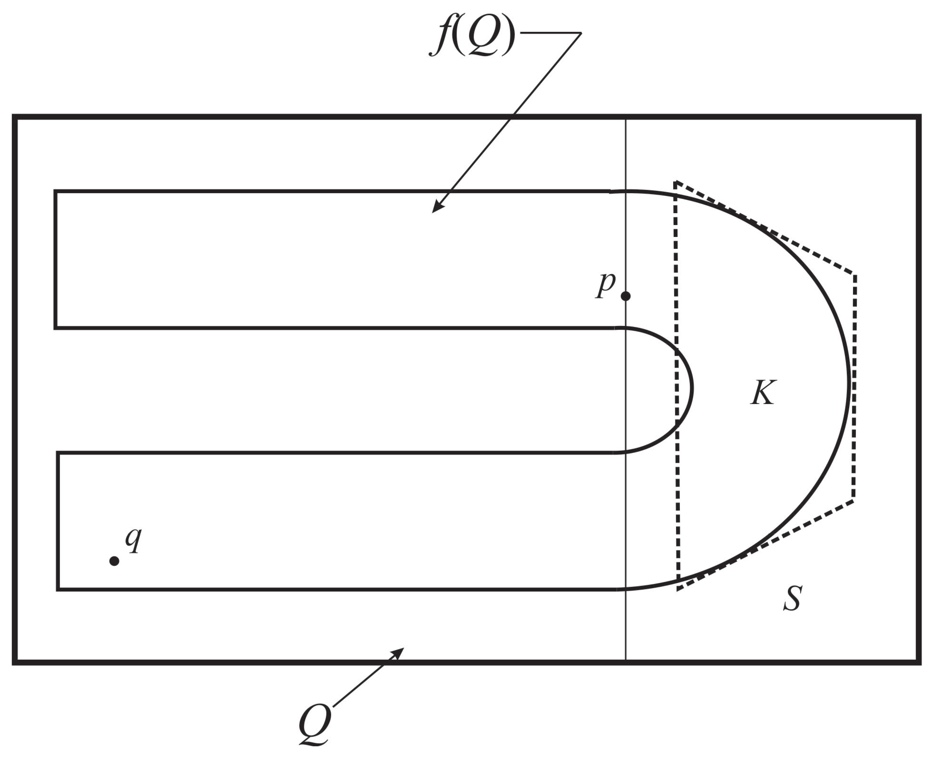
The GAH is a modification of the AH that can be represented as a geometric paradigm with either just one or two fixed points, both of which are saddles. Figure 1 shows a rendering of a GAH with two saddle points, which can be constructed as follows. The rectangle is first contracted vertically by a factor , then expanded horizontally by a factor , and finally folded back into the usual horseshoe shape in such a manner that the total height and width of the horseshoe do not exceed the height and width, respectively, of the trapping rectangle Q. Then, the horseshoe is translated horizontally so that it is completely contained in Q. Obviously, the map f defined by this construction is a smooth diffeomorphism. Clearly, there are also many other ways to obtain this geometrical configuration. For example, the map f as described above is orientation-preserving, and an orientation-reversing variant can be obtained by composing it with a reflection in the horizontal axis of symmetry of the rectangle, or by composing it with a reflection in the vertical axis of symmetry followed by a composition with a half-turn. Another construction method is to use the standard Smale horseshoe that starts with a rectangle, followed by a horizontal composition with just the right scale factor or factors to move the image of Q into Q, while preserving the expansion and contraction of the horseshoe along its length and width, respectively.
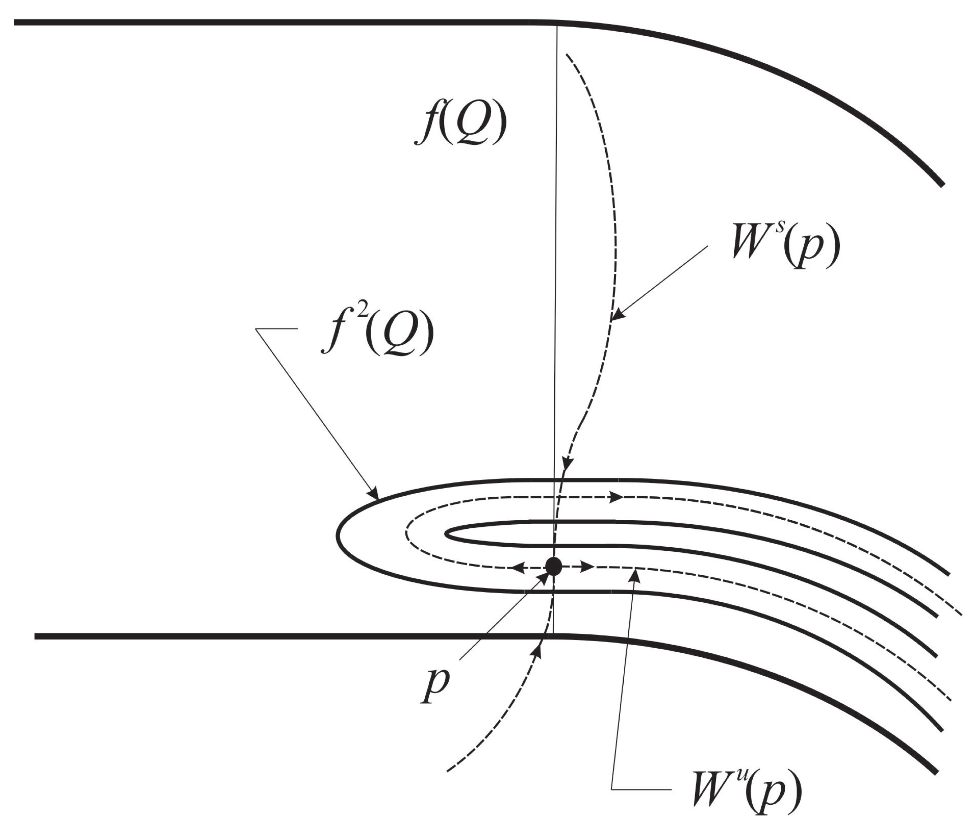
It is important to note that subrectangle S with its left vertical edge through p, which contains the arch of the horseshoe and the keystone region K, plays a key role in the dynamics of the iterates of f. In particular, we require that the map satisfy the following additional property, which is illustrated in Figure 2:
- (★)
- f maps the keystone region K (containing a portion of the arch of the horseshoe) to the left of the fixed point p and the portion of its corresponding stable manifold containing p and contained in .
The definition above and (★) can be shown to lead to the conclusion that
where is the unstable manifold of p, a global chaotic strange attractor (CSA).
The map above can be considered to be the paradigm for a GAH, but there are many analogs. In fact, let be any smooth diffeomorphism of a quadrilateral trapping region possessing a horseshoe-like image with a keystone region containing a portion of the arch of analogous to that shown in Figure 1. Suppose that the map is expanding by a scale factor uniformly greater than one along the length of the horseshoe and contracting transverse to it by a scale factor uniformly less than one-half in the complement of a subset of containing . Then, if F satisfies an additional property analogous to (★), it maps into an open subset of to the left of the saddle point , and
is a global CSA.
3.2. A GAH Producing System
We now construct an ODE in with a Poincaré section that is a GAH. The transversal we use is the following square in the -plane defined in Cartesian and polar coordinates
The trick is to find a relatively simple (necessarily nonlinear) ODE having as a transversal with an induced Poincaré first-return map such that is a GAH. We chose the ODE based upon a rotation about the z-axis so that the square evolves into the GAH as makes a full rotation. The first half of the metamorphosis takes care of the vertical squeezing and horizontal stretching, while the second half produces the folding. It is not difficult to show that the system (in cylindrical coordinates)
flows to
which is the original square in the radial half-plane corresponding to stretched by a factor of 1.2 along the x-axis and squeezed by a factor of 1/5 with respect to along the z-axis in the radial half plane corresponding to . Consequently, (2) produces the first half of the desired result comprising the stretching and squeezing for .
Note that (2) can be integrated directly to obtain the following for and initial condition
Now, we have to attend to the folding for . For this we use a rotation in planes orthogonal to a fixed circle in the -plane. In these planes corresponding to a circle of radius c, given as , we define Euclidean coordinates with origin and corresponding polar coordinates as
where and . Then, when , we take the folding part for to be
or equivalently
It is easy to verify from the above that is constant (call it ) for the solutions of (6) or (7) and that the solution initially (at ) satisfying is
where
The above ((6) or (7)) describes the folding field for and . In order to smoothly fill in the rest of the field, we shall use the function
which can be recast as
We have now assembled all the elements for defining an ODE that generates a GAH Poincaré section. This ODE, which incorporates (2) and (7) and is -periodic in , has the following form:
subject to the initial condition
where
and
Finally, it is not difficult to show that the Poincaré section of the transversal (and trapping region) under the system (12) is a GAH with an image that is simply a symmetric reflection about the vertical axis of the horseshoe in Figure 1. However, it appears that the construction of an electronic circuit simulating (12) would be a rather formidable undertaking, so we selected a simpler system, namely, the Rössler attractor model, which is a mildly nonlinear three-dimensional ODE that has a straightforward circuit realization.
4. Poincaré Maps and Circuit Realization of the Rössler Attractor
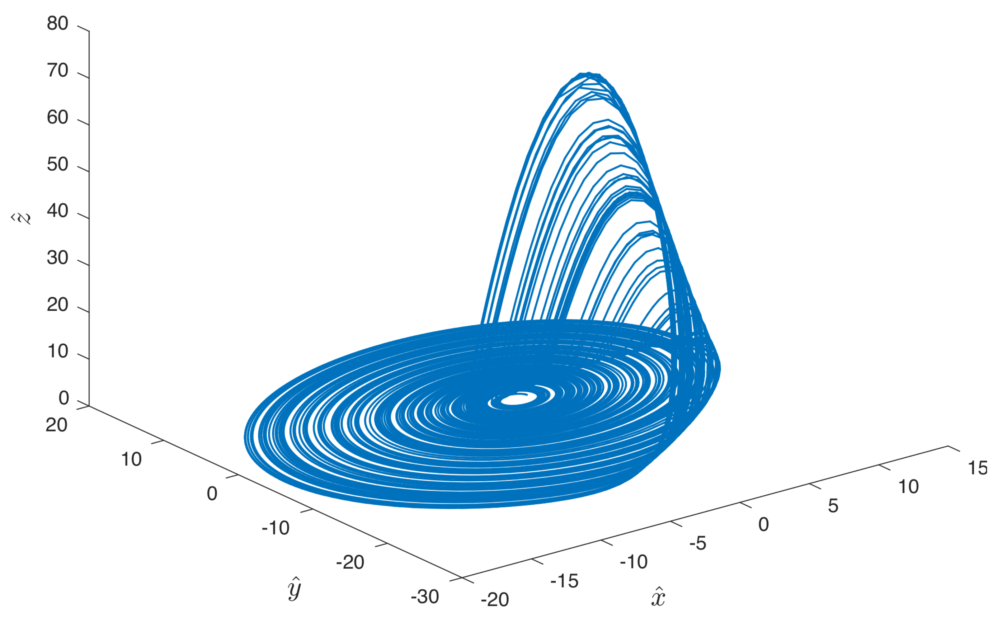
We consider the Rössler attractor
where we use the parameters , , and . This produces the chaotic strange attractor in Figure 3, and it can also be realized by a rather simple electronic circuit.
4.1. The Poincaré Map
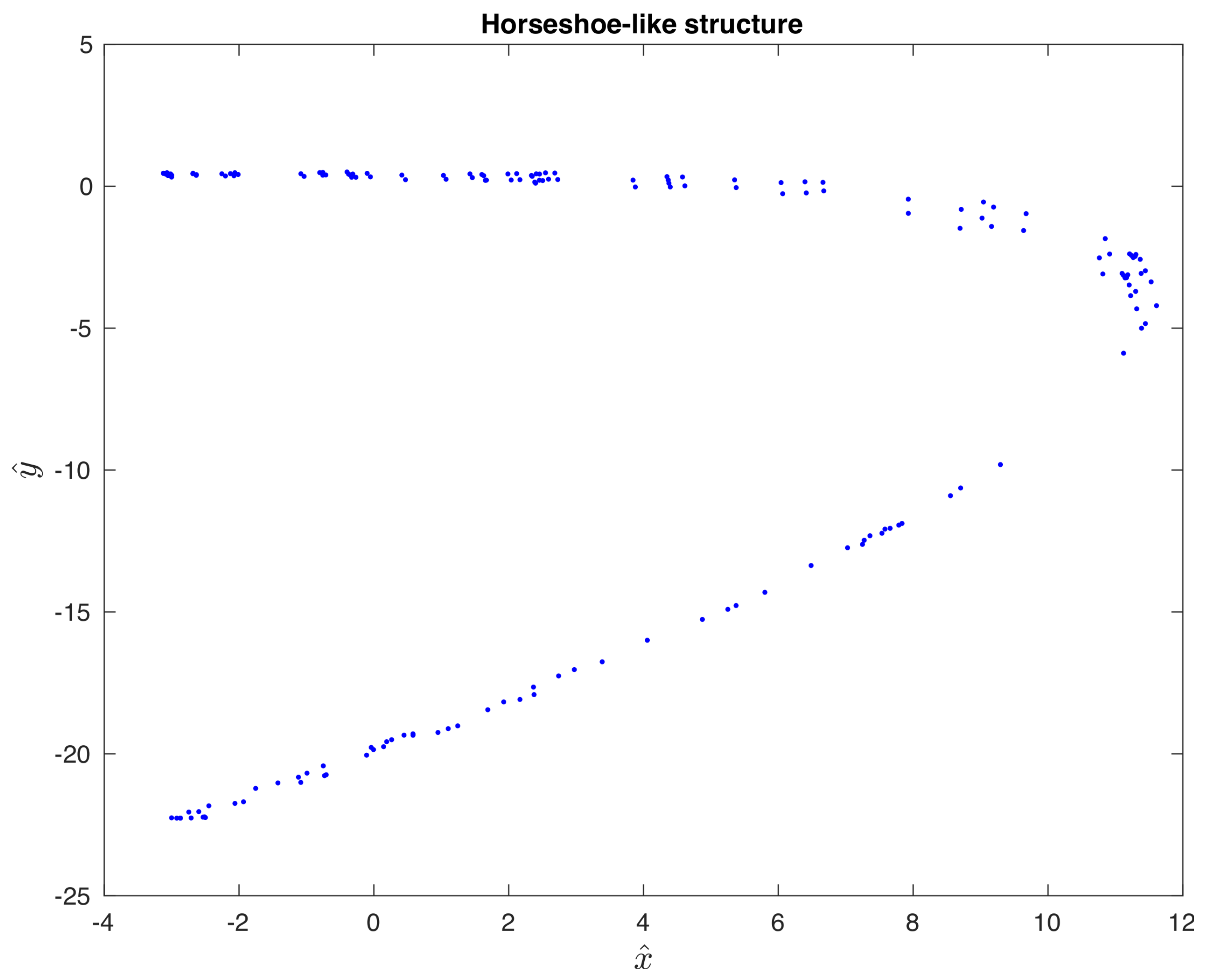
One can use the algorithm in Section 2 to compute any Poincaré section of the attractor; however, what we are particularly interested in is identifying a trapping region for a generalized attracting horseshoe. Assuming the system contains a GAH, we first look for a Poincaré section with a horseshoe-like structure as shown in Figure 4.
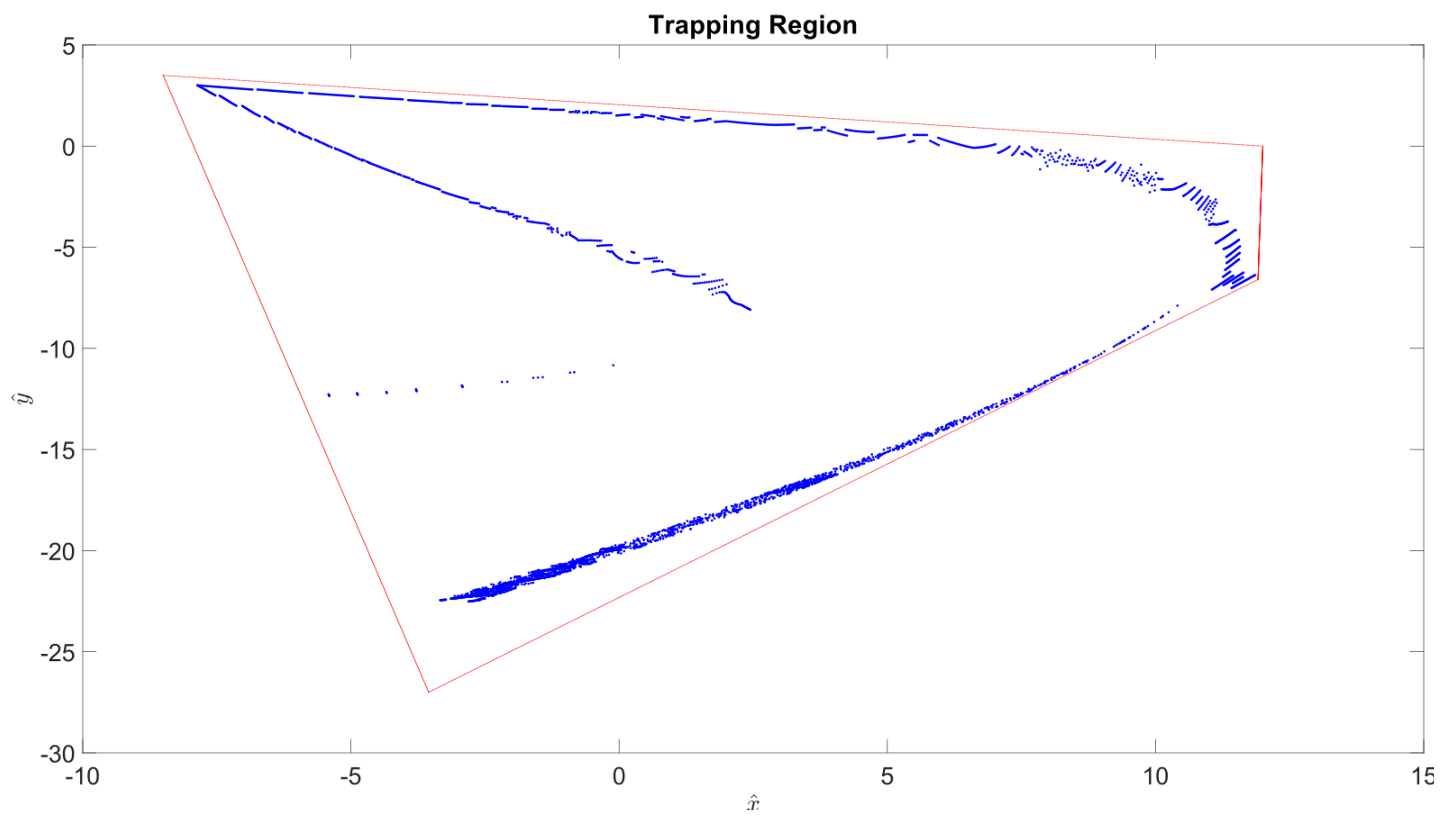
Now, if we can find a rotationally symmetric trapping region around this horseshoe, we shall have shown evidence for the existence of a GAH. First, we identify vertices of a quadrilateral that fully encompasses the horseshoe-like structure. Then, using a recursive algorithm (described in Section 2) we compute the first return map of those vertices on that particular Poincaré section, i.e., the first iteration of the Poincaré map of those points. If the iterates are contained within that quadrilateral, the points on the quadrilateral itself can be tested. In Figure 5, four-thousand points on the quadrilateral are iterated, and it is illustrated that this first return is completely contained in the quadrilateral. While this is not a proof, the grid spacing on the quadrilateral provides compelling evidence that this is a trapping region for the GAH.
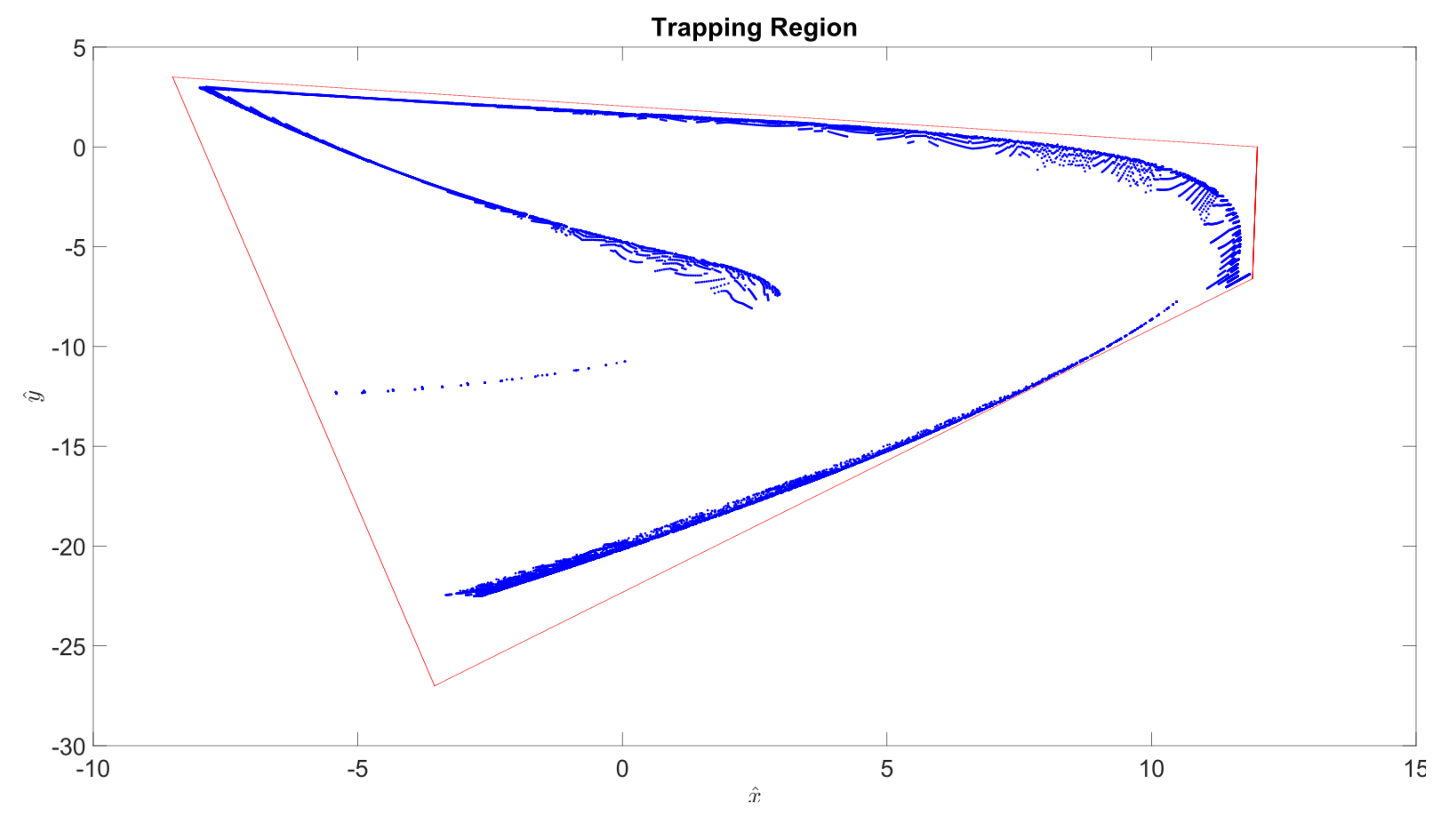
In order to provide more compelling evidence, we compute higher-order iterations of the Poincaré map in Figure 6.
4.2. Circuit Realization of the Rössler System
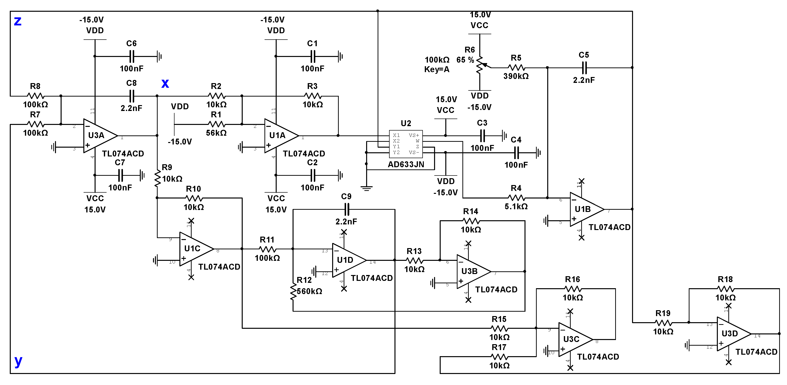
It happens that there are several known examples of electronic circuits realizing the Rössler attractor system. We chose the one, obtained from [11], shown in Figure 7 with a list of components in Table 1.
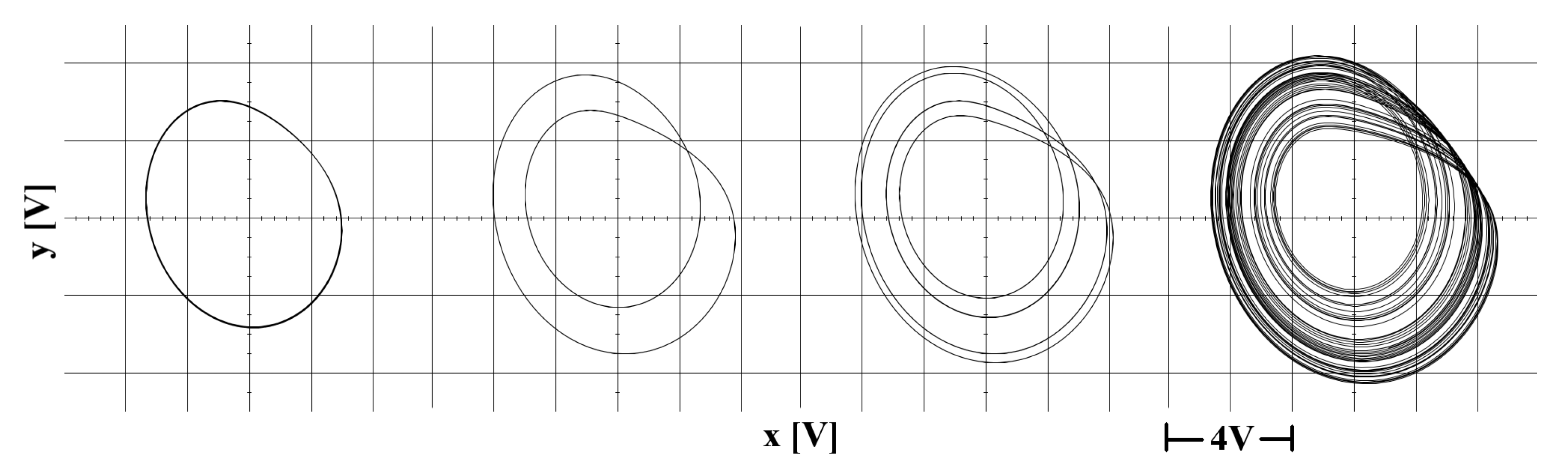
The physical realization of the Rössler attractor circuit was constructed using summing amplifiers, integrators, and a multiplier. Due to the nature of this system, the operational amplifier must operate within volts in order to avoid clipping of the Rössler Attractor output waveform. In this circuit, resistors were used to represent constant values for parameters a and b in (14). A potentiometer was used to vary the parameter value of b in order to observe the bifurcations of the physical system. We first test the circuit on Multisim and observe the aforementioned bifurcations in Figure 8.
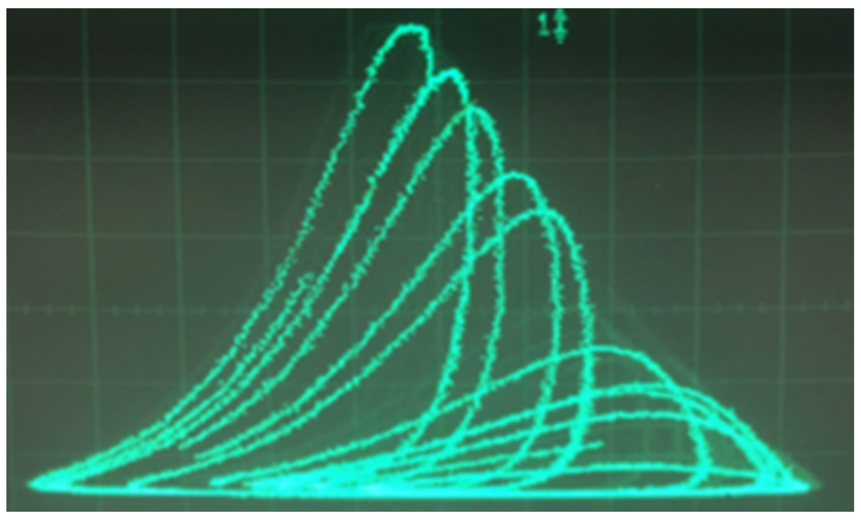
Next, we built the circuit and observed oscilloscope outputs as shown in Figure 9. The Poincaré section that we chose was a particular vertical plane through the top arch of the output shown (see also Figure 3). The acceptable planes were obtained by trial and error via varying the system parameters and rotation of the plane about a vertical axis through the apex of the arc.
5. Potential Applications
One can imagine several practical applications of devices containing electronic circuit realizations of a GAH. Two, which are related to communications and intelligence gathering, immediately come to mind: First, the circuit could be embedded in a communication receiving device, and tuned to certain “static” frequencies different from those in the expected incoming messages. The strong global attracting characteristics of the circuit would separate the static from the incoming messages, thereby enhancing the receiving capabilities of system. In effect, the GAH circuit would filter out the static.
Second, a stationary or compact mobile device incorporating the GAH circuit could be used to penetrate and analyze various communication systems. Either by connecting remotely in the case of a stationary device or directly for a mobile version, the global attracting properties could be employed to extract crucial characteristics of the system to which it is connected. Moreover, the same attracting features of the GAH circuit device could be used to absorb various parts of sent messages that would render them useless, false, or simply misleading.
The two rather basic applications mentioned provide just a glimpse of the possible applications of GAH circuits, most of which would probably be related to information systems, data collection, and filtering. Moreover, there are more applications that could exploit the chaotic strange attractor associated with a GAH circuit. For, example a GAH circuit device could be used either to control chaos, introduce chaos or adjust the fractal dimension of outputs of a variety of applicable processes based on dynamical systems.
Such mechanisms may aid in a variety of fields including cryptography and cyber security. While encryption techniques reliant on the iterate by iterate behavior of chaotic maps have had their short comings due to irreversibly in analog form and a lack of proper security when implemented in software, the global properties of a GAH circuit may provide a useful intermediate stage during various forms of symmetric encryption by allowing a signal of importance to pass both through and around such a subsystem in parallel. Long-term global properties from the signal sent through a GAH circuit can be extracted and used to manipulate the unaltered signal before reaching the recipient, thereby substantially increasing the difficulty of decryption. As the global properties of such a system (i.e., factors taken from its geometry and macro-scale structure) are less influenced by minor imperfections in the circuit, reversing the process becomes far more tangible.
Furthermore, adding to our second practical application claim, a GAH device could prove to have various applications in machine learning, specifically regarding the creation and prevention of adversarial attacks on deep neural networks. By altering carefully chosen properties of the data meant to be received by the network intelligible yet incorrect results can be forced. In the same light, the proper extraction of dominant incoming signals may help prevent the same sort of issue in special cases.
6. Conclusions
We constructed a rather complicated nonlinear three-dimensional ordinary differential equation (ODE) having a Poincaré section that is a GAH map, but it is not particularly amenable to electronic circuit realization, which was a goal of the investigation. Therefore, instead of the initial ODE, we selected the Rössler attractor; a mildly nonlinear three-dimensional ODE that has a reasonably simple circuit realization and can actually produce GAH maps for carefully chosen Poincaré sections. We constructed the corresponding GAH circuit and used a novel iteration procedure to generate good approximations of the chaotic strange attractors associated to the GAH maps. Finally, in addition to the experimental and analytic aspects of our investigation, we discussed a number of potential practical applications of the GAH circuit. Most of the envisioned applications were in the realms of communication and information gathering.
Supplementary Materials
The following are available at https://0-www-mdpi-com.brum.beds.ac.uk/2073-8994/13/1/30/s1.
Author Contributions
Conceptualization, A.R. and D.B.; Formal analysis, K.M.; Investigation, K.M., I.J., P.S. and A.R.; Methodology, A.R.; Project administration, A.R.; Supervision, A.R. and D.B.; Validation, I.J.; Visualization, K.M.; Writing—original draft, A.R. and D.B.; Writing—review & editing, I.J., A.R. and D.B. All authors have read and agreed to the published version of the manuscript.
Funding
This research received no external funding.
Institutional Review Board Statement
Not applicable.
Informed Consent Statement
Not applicable.
Data Availability Statement
All data and computer programs that were developed are included as Supplementary Materials.
Acknowledgments
The authors would like to thank the NJIT Provost Research Grants for funding this research. K.M. was funded by the Provost high school internship, and P.S. was funded by Phase-1 Provost Undergraduate Research Grant, with D.B. as faculty mentor and A.R. as graduate student mentor. K.M. appreciates the support of Bridgewater-Raritan High School, P.S. and I.J. appreciate the support of the Electrical and Computer Engineering Department at NJIT, and A.R. and D.B. appreciate the support of the Department of Mathematical Sciences and the Center for Applied Mathematics and Statistics (CAMS) at NJIT. In addition, K.M., I.J., and A.R. would like to acknowledge their current institutions: K.M. appreciates the support of the Department of Computer Science at UI-UC, I.J. appreciates the support of the Department of Applied Mathematics and Statistics at SU, and A.R. appreciates the support of the Department of Applied Mathematics at UW. Finally, the authors would like to give their sincere thanks to the reviewers for their insightful comments that helped improve the manuscript.
Conflicts of Interest
The authors declare no conflict of interest.
References
- Smale, S. Diffeomorphisms with many periodic points. In Differential and Combinatorial Topology; Carins, S., Ed.; Princeton University Press: Princeton, NJ, USA, 1963; pp. 63–80. [Google Scholar]
- Lorenz, E.N. Deterministic nonperiodic flow. J. Atoms. Sci. 1963, 20, 130–141. [Google Scholar] [CrossRef] [Green Version]
- Rössler, O.E. An equation for continuous chaos. Phys. Lett. A 1976, 57, 397–398. [Google Scholar] [CrossRef]
- Matsumoto, T. A chaotic attractor from Chua’s circuit. IEEE Trans. Circuits Syst. 1984, 31, 1055–1058. [Google Scholar] [CrossRef]
- Hénon, M. A two-dimensional mapping with a strange attractor. Commun. Math. Phys. 1976, 50, 69–77. [Google Scholar] [CrossRef]
- Lozi, R. Un attracteur étrange (?) du type attracteur de hénon. J. Phys. Colloq. 1978, 39, 9–10. [Google Scholar] [CrossRef]
- Blackmore, D.; Joshi, Y. Strange attractors for asymptotically zero maps. Chaos Solitons Fractals 2014, 68, 123–138. [Google Scholar]
- Joshi, Y.; Blackmore, D.; Rahman, A. Generalized attracting horseshoe and chaotic strange attractors. arXiv 2020, arXiv:1611.04133v2. [Google Scholar]
- Rahman, A.; Jordan, I.; Blackmore, D. Qualitative models and experimental investigation of chaotic nor gates and set/reset flip-flops. Proc. Roy. Soc. A 2018, 474, 1–19. [Google Scholar] [CrossRef] [PubMed] [Green Version]
- Gonze, D. poincare.m. Available online: http://homepages.ulb.ac.be/~dgonze/info/matlab/poincare.m (accessed on 25 February 2011).
- Glen, K. Rossler Attractor. Available online: http://www.glensstuff.com/rosslerattractor/rossler.htm (accessed on 25 January 2017).
Figure 1.
A planar GAH with two saddle points.

Figure 2.
Local (transverse) horseshoe structure of near p.

Figure 3.
The Rössler attractor with parameters , , and , and a rotation (represented by and ) of in spherical coordinates.
Figure 3.
The Rössler attractor with parameters , , and , and a rotation (represented by and ) of in spherical coordinates.

Figure 4.
Poincaré section () of the Rössler attractor containing a horseshoe-like structure. Plot is shown in the rotated frame.
Figure 4.
Poincaré section () of the Rössler attractor containing a horseshoe-like structure. Plot is shown in the rotated frame.

Figure 5.
The first return (blue markers) of the quadrilateral trapping region (red markers) with vertices located at . While the quadrilateral edges look “continuous”, it should be noted that it is in fact discretized using four thousand points, which are then mapped back to the Poincaré section (). Plot is shown in the rotated frame with and denoting rotated axes.

Figure 6.
First five iterations of the Poincaré map (blue markers) of the quadrilateral trapping region (red markers) with vertices located at . While the quadrilateral edges look “continuous”, it should be noted that it is in fact discretized using four thousand points, which are then mapped back to the Poincaré section (). Plot is shown in the rotated frame with and denoting rotated axes.

Figure 7.
Multisim circuit diagram for Röossler attractor.

Figure 8.
Multisim outputs of the Rössler attractor showing a period doubling Hopf bifurcation leading to chaos.
Figure 8.
Multisim outputs of the Rössler attractor showing a period doubling Hopf bifurcation leading to chaos.

Figure 9.
Oscilloscope output from Rössler attractor circuit.


Table 1.
List of components for the Röossler attractor circuit.
| Type | Quantity | Code |
|---|---|---|
| 10 k Resistor | 11 | |
| 100 k Resistor | 3 | |
| 390 k Resistor | 1 | |
| 56 k Resistor | 1 | |
| 560 k Resistor | 1 | |
| 5.1 k Resistor | 1 | |
| 100 k Potentiometer | 1 | |
| 100 nF Capacitor | 6 | |
| nF Capacitor | 3 | |
| Op-Amp | 2 | AD633JN |
| Multiplier | 1 | TL074CN |
Publisher’s Note: MDPI stays neutral with regard to jurisdictional claims in published maps and institutional affiliations. |
© 2020 by the authors. Licensee MDPI, Basel, Switzerland. This article is an open access article distributed under the terms and conditions of the Creative Commons Attribution (CC BY) license (http://creativecommons.org/licenses/by/4.0/).
Share and Cite
MDPI and ACS Style
Murthy, K.; Jordan, I.; Sojitra, P.; Rahman, A.; Blackmore, D. Generalized Attracting Horseshoe in the Rössler Attractor. Symmetry 2021, 13, 30. https://0-doi-org.brum.beds.ac.uk/10.3390/sym13010030
AMA Style
Murthy K, Jordan I, Sojitra P, Rahman A, Blackmore D. Generalized Attracting Horseshoe in the Rössler Attractor. Symmetry. 2021; 13(1):30. https://0-doi-org.brum.beds.ac.uk/10.3390/sym13010030
Chicago/Turabian StyleMurthy, Karthik, Ian Jordan, Parth Sojitra, Aminur Rahman, and Denis Blackmore. 2021. "Generalized Attracting Horseshoe in the Rössler Attractor" Symmetry 13, no. 1: 30. https://0-doi-org.brum.beds.ac.uk/10.3390/sym13010030
Note that from the first issue of 2016, this journal uses article numbers instead of page numbers. See further details here.