Fluctuation–Dissipation Relations in Active Matter Systems

Abstract

We investigate the non-equilibrium character of self-propelled particles through the study of the linear response of the active Ornstein–Uhlenbeck particle (AOUP) model. We express the linear response in terms of correlations computed in the absence of perturbations, proposing a particularly compact and readable fluctuation–dissipation relation (FDR): such an expression explicitly separates equilibrium and non-equilibrium contributions due to self-propulsion. As a case study, we consider non-interacting AOUP confined in single-well and double-well potentials. In the former case, we also unveil the effect of dimensionality, studying one-, two-, and three-dimensional dynamics. We show that information about the distance from equilibrium can be deduced from the FDR, putting in evidence the roles of position and velocity variables in the non-equilibrium relaxation.

1. Introduction

The fluctuation–dissipation relations (FDR) played a pivotal role in the development of non-equilibrium statistical mechanics. Starting from the regime of weak departure from equilibrium, with the pioneering work of Einstein on mobility–diffusivity relation, through the central work of Onsager on the reciprocal relations [1], a unification of further theoretical results was obtained in the Kubo’s linear response theory [2], which includes also Green–Kubo relations useful for transport coefficients in spatially extended systems. In Onsager’s and Kubo’s theories, all relations remain “simple”, provided that some kind of time-reversal symmetry holds in the unperturbed state. As soon as this symmetry is lost, the simplicity of linear response and transport coefficients is no more guaranteed [3].

Time-reversal symmetry is broken in widespread natural phenomena: a constraint against equilibration is usually given by non-equilibrium boundary conditions or in the presence of very slow relaxation dynamics, as in glassy systems. Hindrance to equilibration can also be caused by internal non-conservative forces, such as those in granular systems and in self-propelled particles. In all those cases, response theory must be generalized, paying a price in simplicity. Several generalized relations have been proposed in the last decades; they still connect the perturbed system to the unperturbed one, but often require some detailed microscopic knowledge of the system. Some generalized relations may take a simple form in particular situations, e.g., an effective temperature may replace the thermostat temperature in a range of well-separated timescales for aging glassy systems, but this scenario is far from being general [4,5]. More frequently, one faces a situation where the equilibrium FDR is modified by additional contributions of a more complex nature.

The several approaches to FDR present in the literature belong to two main classes: Class A requires the knowledge of the stationary distribution, while class B only requires the knowledge of the microscopic dynamical rules (transition rates or Langevin equations). First examples of FDR of class A were obtained for chaotic systems and Brownian dynamics with non-conservative forces [6,7]. In those cases, the knowledge of the steady-state probability distribution (at least, in some approximations) still maintains a fundamental importance: in the absence of this information the generalized FDR remains, somehow, an implicit relation which can be useful to test ansatz on the steady-state properties [8]. More recent FDR of this kind express the non-equilibrium contributions in terms of stochastic entropy production [9,10]. Examples of FDR of class B are derived from the Malliavin weight sampling [11], or the Novikov theorem [12], which have been intensively employed in the context of glassy physics and represent a powerful tool to calculate the susceptibility and, thus, the so-called effective temperature of a system [4,13]. However, in this approach, the FDR involves correlations with the noise and the physical meaning of these terms remain often difficult to catch. Other schemes in this class include the description in terms of “frenetic” contributions [14,15], focusing on the role of time-symmetric fluctuations out of equilibrium (see also in [16] for derivations of analogous FDR for discrete spin variables).

The generalization of the FDR to active matter represents a challenging issue. Systems of active particles are usually far from equilibrium and many of them move in the solvent through complex mechanisms involving chemical reactions or mechanical agents, such as cilia or flagella [17,18,19,20]. In the spirit of minimal modeling, these systems could be described through simple stochastic dynamics that resembles that of passive colloids except for the addition of a coarse-grained time-dependent force, often called self-propulsion or simply active force [21,22]. This force replaces the microscopic details of the system that, in general, are related to complicate internal mechanisms of energy transduction and involve an intrinsic source of strong deviation from thermodynamic equilibrium. Except for special cases, the steady-state properties of these non-equilibrium models are not known analytically or without approximations, and thus FDR of class A remain in implicit forms [23,24]. Explicit expressions can be worked out in the limit of small persistence time $\tau$, with the first example obtained in [25]. On the other hand, the Malliavin weight sampling procedure has been applied to the case of active particle dynamics [26,27] and, in particular, employed to numerically calculate susceptibility and effective temperature of suspensions of active particles [28,29,30,31,32], even, in phase-separated configurations [33]. We remark that usually the concept of effective temperature is thermodynamically meaningful only in systems with well-separated time-scales [34]. This approach has been also employed to calculate the transport coefficients, such as the mobility, in combination with an approximate method valid at low-density values or small persistence regimes [35,36]. An attempt to generalize FDR to active systems has been recently presented in [15,37,38]: in the latter case, a relation involving a double-time derivative of correlators appears, making the meaning of the formula and its numerical (and experimental) application not immediate.

In this paper, we provide a clear example in the framework of active matter for which a generalized FDR of class B can be explicitly obtained in terms of simple steady-state correlations, involving functions of the observables (such as positions and velocities), which do not require a knowledge of the steady-state properties and do not involve any approximation (e.g., for small persistence regimes, etc.). Moreover, we propose a new quantity to measure the departure from equilibrium, which is defined in terms of the generalized FDR and takes into account the features of the system under time-reversal. We study the behavior of such a quantity for non-interacting self-propelled particles confined via different potentials, ranging from non-harmonic single-well to double-well potentials. In the former case, we also investigate the effect of the dimensionality on the non-equilibrium features.

The article is structured as follows. In Section 2, we introduce model and notations, while in Section 3 we report the FDR relation obtained in our approach. Section 4 is dedicated to the numerical study of the linear response, exploring both convex and non-convex potentials in one-, two-, and three-dimensional systems. Finally, in Section 6, we compare our results with two popular approximated results showing their failure, while the final section is dedicated to discussions and conclusions.

2. Self-Propelled Particles

We consider a well-known scheme to describe the behavior of self-propelled particles, the Active Ornstein–Uhlenbeck (AOUP) model [39,40,41,42,43,44,45,46] (also known as Gaussian Colored Noise (GCN)). The AOUP has been employed to reproduce the phenomenology of passive colloids immersed in a bath of active particles [47,48,49,50] but also—perhaps at a more approximate level—the dynamics of self-propelled particles themselves. Its connection with other popular models for self-propelled particles has been addressed by some authors [51,52]. For instance, the AOUP model can reproduce the accumulation near the boundaries of channels and obstacles [41,53], the non-equilibrium clustering or phase-separation [25,54,55] typical of active matter and the spatial velocity correlation spontaneously observed in dense active systems [56,57]. According to the AOUP scheme, the position in d dimensions $\mathbf{x}$ of the self-propelled particle evolves with the following stochastic equation,

$$\gamma \dot{\mathbf{x}}\left(t\right)=\mathbf{F}\left(t\right)+{\mathbf{f}}_a\left(t\right)+\mathbf{h}\left(t\right),$$

(1)

where $\gamma$ is the drag coefficient. In Equation (1), we have neglected the thermal noise due to the solvent as the thermal diffusion is usually smaller than the effective diffusion due to the active force in several experimental active systems [18]. The term $\mathbf{F}\left(t\right)=-\nabla U\left[\mathbf{x}\right(t\left)\right]$ models the force due to an external confining potential, while the term ${\mathbf{f}}_a\left(t\right)$ represents the self-propulsion of the particle i and is described by an Ornstein–Uhlenbeck process:

$$\tau {\dot{\mathbf{f}}}_a=-{\mathbf{f}}_a+\gamma \sqrt{2D_a}\xi ,$$

(2)

where $\xi$ is a white noise vector with zero average and unit variance. The parameter $\tau$ is the persistence time, while $D_a$ is the diffusion coefficient due to the self-propulsion. Finally, the term $\mathbf{h}\left(t\right)$ is an external small perturbation used to probe the linear response properties of the system. In what follows, the perturbed dynamics will be denoted by the superscript h to be distinguished by the unperturbed one. The response function can be computed as the observed (normalized) variation of some observable when the perturbation is an impulse at time 0, i.e., $\mathbf{h}\left(t\right)=\gamma \delta \mathbf{x}\left(0\right)\delta \left(t\right)$ (with $\delta \mathbf{x}\left(0\right)$ a vector with infinitesimal displacements representing the impulsive perturbation). In general, with the exception of singular measures, it is possible to derive a compact formula for the response function of one of the degrees of freedom $x_i$ of the system to the perturbation of a degree of freedom $x_j$, ${\mathcal{R}}_{x_i{x}_j}$, defined—in the steady state—as

$${\mathcal{R}}_{x_i{x}_j}\left(t\right)=\frac{{\langle x_i\left(t\right)\rangle }^h-\langle x_i\left(t\right)\rangle }{\delta x_j\left(0\right)}=\gamma {\left.\frac{\delta {\langle x_i\left(t\right)\rangle }^h}{\delta h_j\left(0\right)}\right|}_{h=0},$$

(3)

where $t>0$ and, in the last equality, we have introduced the functional derivative with respect to the perturbative force $h_j\left(0\right)$. In the following, for the one-dimensional case, we will replace ${\mathcal{R}}_{xx}\left(t\right)$ with ${\mathcal{R}}_x\left(t\right)$ for notational convenience.

3. Generalized Fluctuation–Dissipation Relation for Self-Propelled Particles

The model introduced so far reaches a non-equilibrium stationary state even in the absence of perturbation displaying a non-vanishing entropy production [25,58,59,60], with a few special exceptions: in the absence of external potential, or in the presence of linear forces, the detailed balance is restored and the system recovers an apparent equilibrium state with vanishing entropy production [61]. This is an imperfection of the AOUP model [62]. Except for these special cases, the probability distribution, $p(\mathbf{x},{\mathbf{f}}_a)$, is unknown. An approximation can be obtained, valid in the proximity of equilibrium ($\tau =0$) [25,43,61,63]. Therefore, in general, this model of self-propelled particles cannot be treated within the FDR of class A, because the FDR remains implicit:

$${\mathcal{R}}_{x_i{x}_j}\left(t\right)=-〈x_i\left(t\right)\frac{\partial }{\partial x_j}log\left[p(\mathbf{x}\left(0\right),{\mathbf{f}}_a\left(0\right))\right]〉,$$

(4)

where the average $\langle ·\rangle$ is obtained considering the unperturbed system and $p(\mathbf{x},{\mathbf{f}}_a)$ is the stationary probability distribution in the absence of perturbations that depends on the whole set of particle positions and velocities. Equation (4) can be used only perturbatively in powers of the persistence time since the expression of $p(\mathbf{x},{\mathbf{f}}_a)$ is only known perturbatively in powers of $\tau$ [23]. For small $\tau$, the system is near the equilibrium, and, thus, the relation (4) is restricted to the same regimes. A similar approach has been employed in [25].

We propose an alternative approach, inspired by FDR of class B, to calculate the response function in terms of suitable steady-state correlations. Below, we report the final outcome of our technique applied to an AOUP confined by an external potential, while the detailed calculations are accurately described in Appendix A:

$$\begin{array}{cc}\hfill D_a\gamma {\mathcal{R}}_{x_i{x}_j}\left(t\right)=& \frac{1}{2}\left[〈x_i\left(t\right){\nabla }_{j}U\left(0\right)〉+〈{\nabla }_{i}U\left(t\right)x_j\left(0\right)〉\right]\hfill \\ & +\frac{{\tau }^2}{2}\left[〈v_k\left(t\right){\nabla }_k{\nabla }_{i}U\left(t\right)v_j\left(0\right)〉+〈v_i\left(t\right){\nabla }_j{\nabla }_{k}U\left(0\right)v_k\left(0\right)〉\right],\hfill \end{array}$$

(5)

where all the correlations have been evaluated in the steady state and we have introduced the particle velocity $v_j={\dot{x}}_j$. According to our notation, repeated indices are summed: $U\left(s\right)=U\left(\mathbf{x}\right(s\left)\right)$ and ${\nabla }_i={\partial }_{x_i}$. Let us comment in detail on Equation (5): first, we observe that it is symmetric under time reversal (i.e., when times t and 0 are swapped) and involves both position and velocity correlations. The first line of Equation (5) has the same form of the equilibrium FDR holding for passive particles. Indeed, when the detailed balance condition holds (for $\tau \to 0$), the first and the second terms on the right-hand side of Equation (5) coincide, while the second line disappears in such a way that $D_a\gamma {\mathcal{R}}_{x_i{x}_j}=〈x_i\left(t\right){\nabla }_{j}U\left(0\right)〉$. The second line provides two additional terms that are specific non-equilibrium contributions to the response function. Remarkably, these non-equilibrium correlations involve the particle velocity, without containing direct simple dependence on the perturbed observable, namely, the particle position (but of course position is involved through the potential). At variance with the well-known equilibrium scenario, in active systems, ${\mathcal{R}}_{x_i{x}_j}\left(t\right)$ is not only determined by a time correlation involving the position but is strongly affected by the correlations between the other variables involved in the dynamics, the velocity in this case. The harmonic case—which is a special case where the AOUP model satisfies the detailed balance even when $\tau >0$—is treated in Appendix B.

Understanding what are the leading terms in Equation (5) is a challenging issue that cannot be performed in general but requires a numerical analysis. In addition, as the detailed balance does not hold in systems of active particles, in general, the reversibility is broken by the presence of non-zero steady-state currents that produce non-vanishing entropy. The structure of Equation (5) suggests a way to measure how much the system is far from equilibrium by quantifying the unbalance between the couples of terms, to see the effect of irreversibility on the response function. Therefore, we define

$$\begin{array}{cc}\hfill & D_a\gamma {\mathcal{D}}_{ij}^x\left(t\right)=〈x_i\left(t\right){\nabla }_{j}U\left(0\right)〉-〈{\nabla }_{i}U\left(t\right)x_j\left(0\right)〉\hfill \end{array}$$

(6)

$$\begin{array}{cc}\hfill & D_a\gamma {\mathcal{D}}_{ij}^v\left(t\right)={\tau }^2〈v_k\left(t\right){\nabla }_k{\nabla }_{i}U\left(t\right)v_j\left(0\right)〉-{\tau }^2〈v_i\left(t\right){\nabla }_j{\nabla }_{k}U\left(0\right)v_k\left(0\right)〉,\hfill \end{array}$$

(7)

where all the correlations are calculated in the steady state. $D_{ij}^x\left(t\right)$ and $D_{ij}^v\left(t\right)$ vanish at the initial time, $t=0$ and for any t in any equilibrium configurations where the detailed balance holds. For notational convenience, we replace $D_{ij}^x$ and $D_{ij}^v$ with $D_x$ and $D_v$ in the one-dimensional case.

4. Numerical Results

In this section, we numerically check the FDR (5), in two typical cases that cannot be analytically solved: (A) the quartic potential and (B) the double-well potential. On the one hand, (A) represents the simpler convex case of study, except for the harmonic confinement where correlation functions and responses can be analytically computed. In the harmonic case, we remark that the expression (5) is consistent with previous results [23,64] that, in particular, predict an exponential time-decay of the response function with a typical time $\gamma /k$ (see the Appendix B). In this simple case, the response function does not show any dependence on the parameters of the active force. On the other hand, (B) is the simpler non-convex case able to reveal the interplay between the self-propulsion and the non-convex curvature of the potential. This feature has already manifested many dynamical anomalies leading to the emergence of regions with effective negative mobility in the large persistence regime [65] showing a bifurcation-like behavior with non-local stationary probability distribution [66]. In the quartic case, we also unveil the role of the dimensions comparing the results for one-, two-, and three-dimensional systems.

The numerical study is performed keeping $D_a$ and the potential strength fixed, to investigate the role of the persistence time, $\tau$. Time is measured in units of a typical time $t^{*}$, ruling the relaxation of the response function for the passive system (obtained for $\tau \to 0$), which is chosen as a reference case. In particular, $t^{*}=\gamma /k$ for the harmonic potential and $t^{*}=1/\sqrt{D_{a}k}$ for the quartic case. In all the cases, the system is perturbed via a small force along the x-axis, with amplitude $\delta x={10}^{-3}$. This choice guarantees the linear regime of the response calculated using Equation (3).

4.1. Quartic Potential

4.1.1. One-Dimensional System

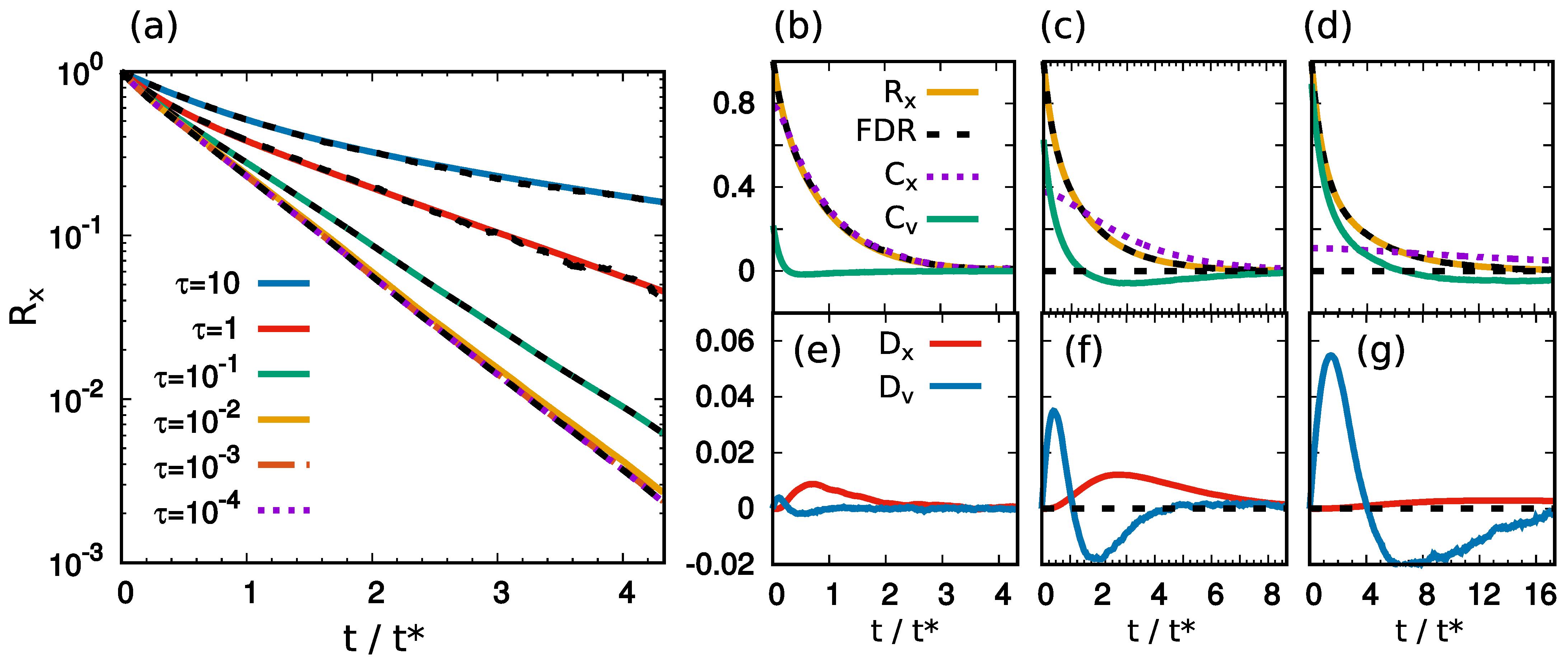
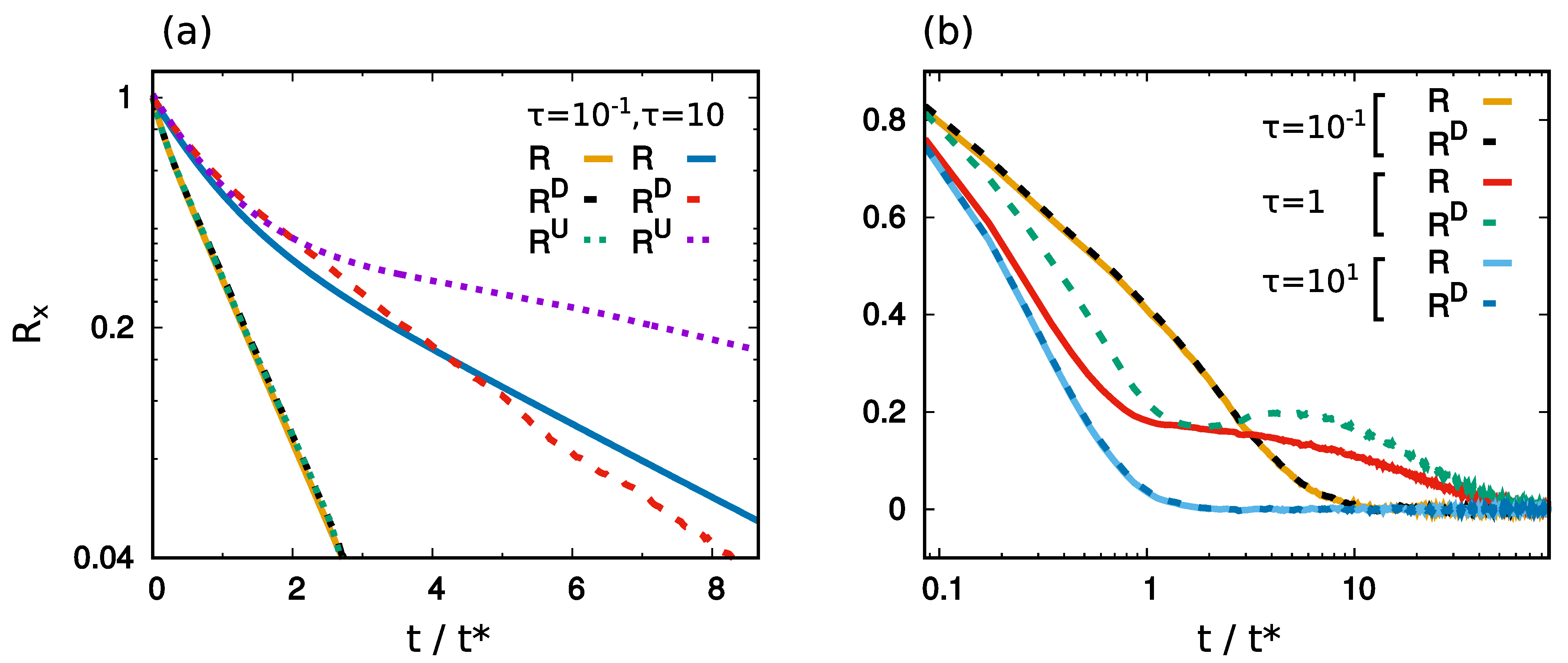
Figure 1a shows the response function, ${\mathcal{R}}_x$, in the case of a quartic potential, $U\left(x\right)=k{x}^4/4$ for several values of $\tau$ exploring both the small and the large persistence regime, i.e., the near and far equilibrium regimes, respectively. The figure reveals the agreement between ${\mathcal{R}}_x\left(t\right)$ calculated from its definition, given by Equation (3), and using the correlation functions appearing in Equation (5) adapted to the one-dimensional case. This numerically confirms the extension of the FDR to AOUP active particles, even far from equilibrium. Specifically, in the small $\tau$ regime, the different curves of ${\mathcal{R}}_x\left(t\right)$ collapse onto the same curve that corresponds to the response function of a passive Brownian particle at temperature $D_a\gamma$. Instead, in the large $\tau$ regime, the larger is $\tau$ the slower is the relaxation of the response function, ${\mathcal{R}}_x\left(t\right)$, that roughly displays two decay regimes. Indeed, it is known that AOUP in a single-well non-harmonic potential accumulates far from the potential minimum roughly near the points where the active force is balanced by the external one, in such a way that the spatial density shows two symmetric peaks [67]. Somehow, the system behaves as if an effective double-well confinement control the particle dynamics, an effect captured by many approximated results [67]. In the quartic case, the $\tau$-dependence is a non-equilibrium consequence caused by the interplay between the nonlinearity of the potential and the persistence of the active force. Indeed, in the harmonic case, the response is $\tau$-independent and uniquely determined by the relaxation time of the potential [64], namely, $t^{*}=k/\gamma$.

In Figure 1b–g, the terms of the FDR (Equation (5)) are separately studied and compared with ${\mathcal{R}}_x\left(t\right)$, for different values of $\tau ={10}^{-1},1,10$, respectively. As emerges from Figure 1b–d, the equilibrium terms, $D_a\gamma C_x\left(t\right)=\langle x\left(t\right)U^{\prime }\left(0\right)\rangle +\langle U^{\prime }\left(t\right)x\left(0\right)\rangle$, are dominant in the near-equilibrium configurations, for small values of $\tau$. In these cases, the non-equilibrium velocity correlations, i.e., $D_a\gamma C_v\left(t\right)={\tau }^2\langle v\left(t\right)U^{″}\left(0\right)v\left(0\right)\rangle +{\tau }^2\langle v\left(t\right)U^{″}\left(t\right)v\left(0\right)\rangle$, only weakly affect the first time decay of ${\mathcal{R}}_x\left(t\right)$ also vanishing approximatively at $t\sim \tau$. When $\tau$ is increased, the contribution of the velocity correlation starts growing even if its decay remains roughly determined by $\tau$, while the potential correlation decreases slowly. Interestingly, the velocity correlation reaches negative values and increases very slowly towards zero almost balancing the potential correlation, as shown in Figure 1b–d. The term $D_a\gamma C_v\left(t\right)={\tau }^2\langle v\left(t\right)U^{″}\left(0\right)v\left(0\right)\rangle +{\tau }^2\langle v\left(t\right)U^{″}\left(t\right)v\left(0\right)\rangle$, becomes dominant in the large persistence regime, as shown in Figure 1b–d, while the term $D_a\gamma C_x\left(t\right)=\langle x\left(t\right)U^{\prime }\left(0\right)\rangle +\langle U^{\prime }\left(t\right)x\left(0\right)\rangle$ gives a negligible contribution.

Finally, to understand the role of the detailed balance violation in the temporal decay of the response, we plot the terms ${\mathcal{D}}_x\left(t\right)$ (solid red lines) and ${\mathcal{D}}_v\left(t\right)$ (solid blue lines), in Figure 1e–g. If these two terms are close to zero, then the detailed balance holds. As expected, this occurs for small $\tau$, while the detailed balance is strongly violated as far as $\tau$ is increased. Moreover, the irreversibility manifests in different ways: ${\mathcal{D}}_x\left(t\right)$ is positive and reaches a peak for $t\sim \tau$, while ${\mathcal{D}}_v\left(t\right)$ shows an oscillation from positive to negative values. As a final remark, the violation of the detailed balance strongly suggests that any equilibrium-like approaches that assume this condition, such as the Unified Colored Noise approximation (that will be explicitly evaluated in Section 5), cannot work in the large persistence regime.

4.1.2. Higher-Dimensional Systems

We explore the role of the system dimensions, both on response functions and FDR. In the case of harmonic confinement (in equilibrium both for dimensions $d=1,2,3$), where the detailed balance holds, the dimensions of the system do not affect the time-decay of the response function.

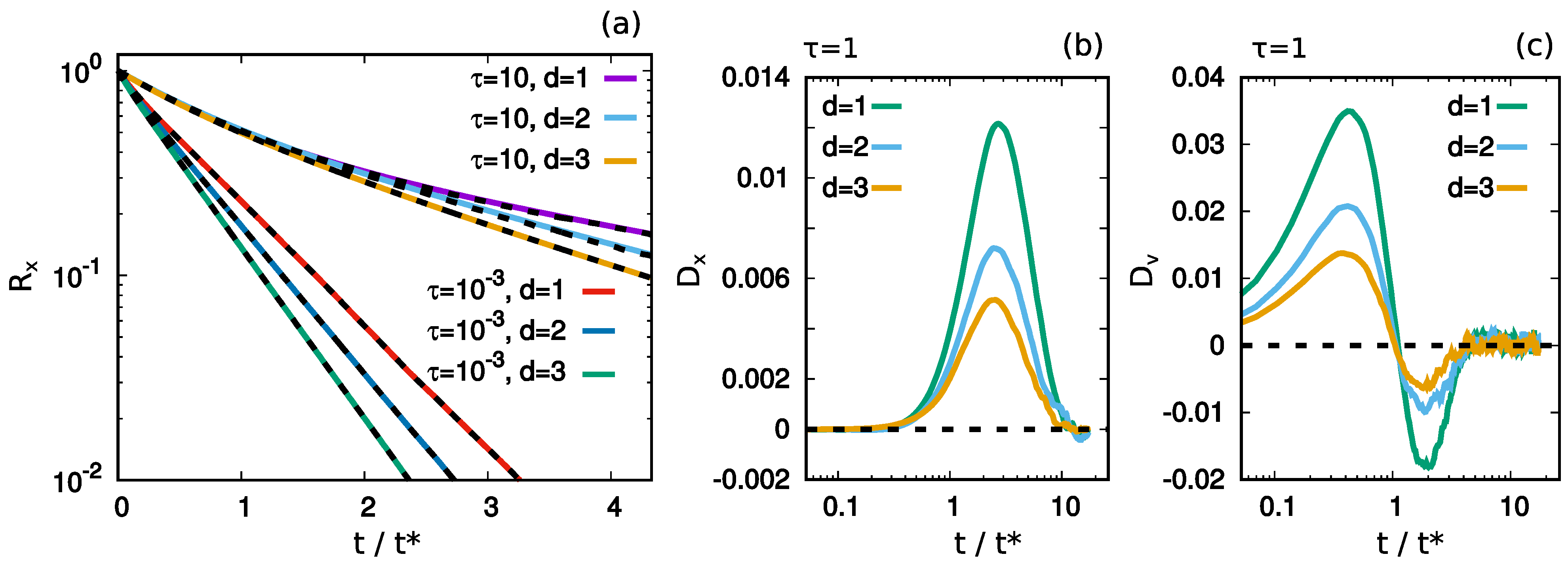
In Figure 2a, we compare ${\mathcal{R}}_x\left(t\right)$ for one-, two-, and three-dimensional self-propelled particles confined through the quartic potentials, $U\left(\mathbf{x}\right)={k\left|\mathbf{x}\right|}^4/4$. We explore both the small and the large persistence regime reporting two reference cases, $\tau ={10}^{-3},10$, respectively. In the small persistence regime ($\tau ={10}^{-3}$) that roughly coincides with the passive case, the larger is the dimension the faster is the decay of ${\mathcal{R}}_x\left(t\right)$, an effect that is entirely due to the nonlinearity of the potential. The increase of the system dimensions increases the effective trapping of the particle because of the confinement, an effect not related to the active force. Instead, in the large persistence regime ($\tau =10$), the correlations show a first temporal decay which does not depend on the dimension of the system (that coincides for $d=1,2,3$), while, in the second stage of the decay, the higher-dimensional systems decrease faster than their corresponding in lower dimensions. Somehow, the active force can suppress the dimensional dependence of the response function, at least for a small time-window.

Figure 2b,c shows the functions ${\mathcal{D}}_x\left(t\right)$ and ${\mathcal{D}}_v\left(t\right)$ for $d=1,2,3$ at $\tau =1$, for simplicity. We highlight that results are similar for other values of $\tau$ (not shown). The qualitative functional forms of $D_x\left(t\right)$ and $D_v\left(t\right)$ are unchanged with d, resembling the shape described in the one-dimensional system: a single peak around $t\sim \tau$ for ${\mathcal{D}}_x\left(t\right)$ and an oscillation from positive to negative values for ${\mathcal{D}}_v\left(t\right)$. The higher is the dimension of the system, the smaller the maximal amplitude of both ${\mathcal{D}}_x\left(t\right)$ and ${\mathcal{D}}_v\left(t\right)$ is. This means that the increase of d, somehow, reduces the breaking of the detailed balance, producing smaller currents. This is also consistent with the increasing difficulties to observe collective phenomena when the dimensions are increased, that in three dimensions typically require larger values of the active forces compared to two-dimensional systems [68].

Finally, let us mention that in the considered cases the cross-terms in the response function, $R_{xy}\left(t\right)=R_{yx}\left(t\right)$, vanish due to symmetry reasons. Indeed, on the one hand, $R_{xy}\left(t\right)$ is an odd function of every cartesian component of position and velocity appearing in the FDR if U is a central potential. On the other hand, the dynamics is invariant for a change of sign for each cartesian component of position and velocity, and thus the same invariance still holds for the response matrix. As a consequence, the only possibility is that $R_{xy}\left(t\right)=0$.

4.2. Double-Well Potential

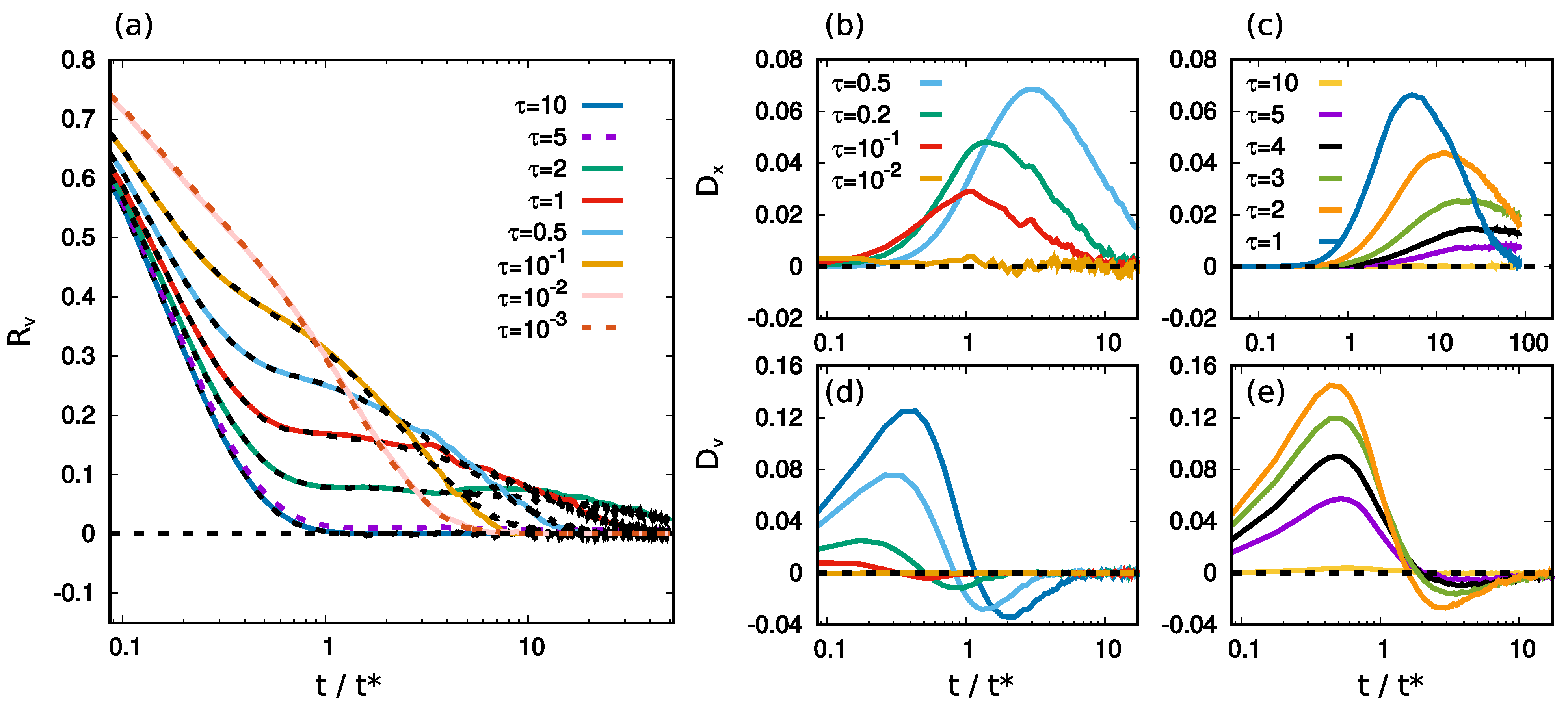
The response function, in the double-well potential case, $U\left(x\right)=k(x^4/4-x^2/2)$, is reported in Figure 3a for different values of $\tau$, exploring both the small and the large persistence regimes. In the small persistence regime, ${\mathcal{R}}_x\left(t\right)$ are collapsed onto the same curve for a broad range of $\tau$ (for $\tau \le {10}^{-2}$). As also occurs in the quartic potential case, the activity is the faster degree of freedom and can be approximated by a white noise, $f_a\approx \sqrt{2D_a}\xi$, so that $\tau$ does not play any role. In this case, the relaxation towards zero is mainly determined by two time regimes, as usual in the case of passive Brownian particles. The first is determined by the relaxation towards the minimum of one of the two wells, and the second accounts for the jump from a well to another. When $\tau$ is increased, the first time regime starts decreasing faster while the second time regime decays more slowly approaching zero for very larger times $t/t^{*}\gg \tau$. Moreover, the increase of $\tau$ also reduces the role played by the second time regime in the temporal decay of ${\mathcal{R}}_x\left(t\right)$ (the larger $\tau$, the smaller the value of ${\mathcal{R}}_x\left(t\right)$ when the second time regime starts occurring). The second time regime is even suppressed when $\tau$ is sufficiently large ($\tau \ge 5$, with the potential setting employed in Figure 3a). This suppression is consistent with the result reported by Fily [69] in the infinite persistence regime where the steady-state density distribution exactly vanishes in the regions where the potential is concave (meaning that no jumps occur). More generally, the statistical relevance of the second time-regime decreases with the increase of the persistence time since the jumps from a minimum to the other occurs rarely when $\tau$ is increased both in the small $\tau$ regime [70,71,72] and in the large $\tau$ regime [66].

As occurs in the case of the quartic potential, the time-decay of ${\mathcal{R}}_x\left(t\right)$ is dominated by the positional correlation or the velocity correlations, in the small and large persistence regimes, respectively (not shown). In Figure 3b–e, we report ${\mathcal{D}}_x\left(t\right)$ and ${\mathcal{D}}_v\left(t\right)$ for different values of $\tau$, revealing an interesting scenario. In analogy with the quartic potential case, the ${\mathcal{D}}_x\left(t\right)$ assumes positive values via a single peak that shifts for larger $t/t^{*}$ when $\tau$ is increased. The ${\mathcal{D}}_v\left(t\right)$ displays an oscillation around zero similarly to the quartic potential case. In a first range of $\tau$, the amplitudes of both ${\mathcal{D}}_x\left(t\right)$ and ${\mathcal{D}}_v\left(t\right)$ increase with $\tau$ (as shown in panels (b,d)). A further increase of $\tau$ (panels (d,e)) produces the amplitude decrease of both ${\mathcal{D}}_x\left(t\right)$ and ${\mathcal{D}}_v\left(t\right)$, until both the functions become flat, approximatively for $\tau \ge 10$. This non-monotonic behavior with the persistence time implies that the system shows an optimal value of $\tau$ that maximizes the departure from the equilibrium via the breaking of the detailed balance. We justify this non-monotonic behavior through the phenomenology reported in [65]. When the particle moves close to one of the two minima, the particle explores a near-equilibrium regime where the local detailed balance almost holds and the local currents are almost zero both in the small and large persistence regimes. This explains why, in this space region, effective equilibrium approaches (that assume the detailed balance condition) give good predictions for the local steady-state properties. Instead, when the particle overcomes the inflected point of the potential (for which ${\partial }_x^{2}U=0$), the particle enters into a non-equilibrium region that, in the large persistence regime, displays an effective negative mobility. There, the particle velocity increases exponentially in time (with very small fluctuations) until the second minimum is reached through an accelerated motion. Thus, most of the non-equilibrium currents are generated when the particle jumps. As we already discussed, the number of jumps from a minimum to the other decreases with $\tau$ (in particular, until to be suppressed for $\tau =10$ and our setting of the potential). Our measure of $D_x$ and $D_v$ confirms that the detailed balance is mostly broken when the jumps occur, and thus it is reasonable to assume that the detailed balance is almost restored for $\tau$ large enough where no jumps occur.

4.3. Measuring the Non-Equilibrium in Active Systems

The study of the correlations and, in particular, the time behavior of ${\mathcal{D}}_x\left(t\right)$ and ${\mathcal{D}}_v\left(t\right)$ suggest introducing a measure to quantify the breaking of the detailed balance and, thus, how much the system is far from equilibrium. As ${\mathcal{D}}_v\left(t\right)$ (and, in principle, also ${\mathcal{D}}_x\left(t\right)$) could assume negative values, we need to consider $|{\mathcal{D}}_v\left(t\right)|$ and $|{\mathcal{D}}_x\left(t\right)|$. We propose a measure based on the time integral of these observables and introduce the quantity:

$$\mu ={\mu }_x+{\mu }_v,$$

(8)

where

$$\begin{array}{cc}\hfill {\mu }_x& =\frac{1}{t^{*}}{\int }_0^{\infty }\left|{\mathcal{D}}_x\left(s\right)\right|ds\hfill \end{array}$$

(9)

$$\begin{array}{cc}\hfill {\mu }_v& =\frac{1}{t^{*}}{\int }_0^{\infty }\left|{\mathcal{D}}_v\left(s\right)\right|ds,\hfill \end{array}$$

(10)

where $t^{*}$ is the typical time that rules the relaxation of the response function for the passive case (see above Section 4). The observable $\mu$ has the following meaning: starting from an initial configuration (which is averaged), $\mu$ measures (i) how much the system is far from the equilibrium during the whole trajectory history, and (ii) the global impact of the detailed balance breaking on the time-decay of the response function. Indeed, when the detailed balance holds, both ${\mu }_x$ and ${\mu }_v$ vanish as $D_x\left(s\right)=D_v\left(s\right)=0$. In general, the larger is $\mu$, the greater is the amount and how long the detailed balance has been broken starting from an initial configuration.

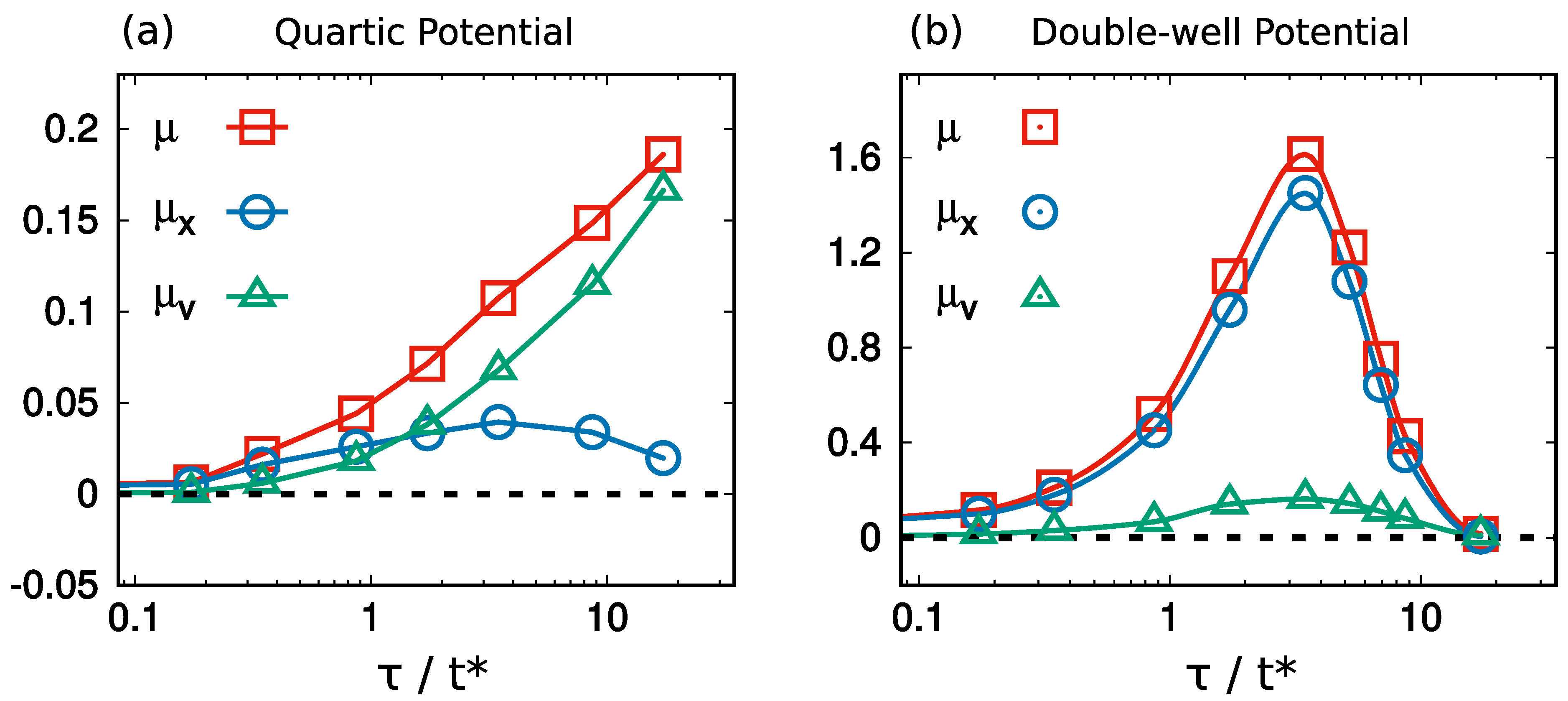
These observables are shown in Figure 4a,b for the quartic and double-well potentials, respectively, for different values of $\tau /t^{*}$. In the quartic potential case, $\mu$ is an increasing function of $\tau$ meaning that the persistence of the activity increases the departure from the equilibrium. While $\mu \approx {\mu }_x$ in the small persistence regime, this is no longer true in the large persistence regime where $\mu \approx {\mu }_v$. The double-well potential case confirms the non-monotonic behavior already observed in Figure 3b–e: $\mu$ shows a peak and then starts decreasing for larger values of $\tau$ until to become almost zero. Moreover, $\mu$ is mainly determined by ${\mu }_x$ for the whole set of $\tau$ values. Indeed, even if $D_v\left(t\right)$ assumes also larger value than $D_x\left(t\right)$, it is different from zero just for a narrow initial time-window while $D_x\left(t\right)$ remains larger for a longer time.

5. Failure of the Approximated Approaches

To provide a qualitative explanation of several phenomena typical of active matter, such as particle accumulation near boundaries or the dynamics in confining potentials, different approximation schemes have been successfully introduced. Among the others, the Unified Colored Noise approximation (UCNA) has been crucial for theoretical purposes, providing the first analytical results for the probability distribution function of both interacting and non-interacting confined systems [73]. This approach provides a scheme to replace the self-propulsion with effective interactions and is quite similar to the so-called Fox approximation [74]. Moreover, it is derived assuming vanishing currents and, thus, the detailed balance, providing the best equilibrium-like predictions to describe the AOUP non-equilibrium dynamics.

Despite the fact that these approaches are very useful to understand the static properties of self-propelled particles, at least when confined through convex potentials or interacting through convex interactions, it has been shown that they fail to describe the active time-dependent properties, such as time correlations and response functions. This concept has been already stressed in [23], where the authors show that the UCNA approximation is able to reproduce the response function just in small persistence regimes, where the system is near the equilibrium and a generalized FDR could be obtained perturbatively in $\tau$ using Equation (4). In the large persistence regime, the numerical study for nonlinear potentials shows the failure of the UCNA approach.

The aim of this Section is to enforce this idea, through additional analytical arguments, showing that the breakdown of the detailed balance plays an important role in correlations and response functions and, as a consequence, also for susceptibility and effective temperature.

5.1. Assuming the Detailed Balance

A possible approximated approach could consist in assuming the detailed balance condition in Equation (5). This choice means that ${\mathcal{D}}_x\left(t\right)=0$ and ${\mathcal{D}}_v\left(t\right)=0$ and should lead to results similar to those obtained in the UCNA approximation. Thus, the following relations hold,

$$\begin{array}{cc}& 〈x_i\left(t\right){\nabla }_{j}U\left(0\right)〉=〈{\nabla }_{i}U\left(t\right)x_j\left(0\right)〉\hfill \end{array}$$

(11)

$$\begin{array}{cc}& 〈v_k\left(t\right){\nabla }_k{\nabla }_{i}U\left(t\right)v_j\left(0\right)〉=〈v_i\left(t\right){\nabla }_i{\nabla }_{k}U\left(0\right)v_j\left(0\right)〉,\hfill \end{array}$$

(12)

in such a way that the response can be approximated by

$${\mathcal{R}}_{x_i{x}_j}^D\left(t\right)\approx \frac{1}{D_a}〈x_i\left(t\right)\frac{{\nabla }_{j}U\left(0\right)}{\gamma }〉+\frac{{\tau }^2}{D_a}〈v_k\left(t\right)\frac{{\nabla }_k{\nabla }_{i}U\left(t\right)}{\gamma }{v}_j\left(0\right)〉,$$

where the superscript D stands for detailed balance. Using the property $\langle v_k\left(t\right){\nabla }_k{\nabla }_{i}U\left(t\right)v_j\left(s\right)\rangle =-d/dt\langle v_k\left(t\right){\nabla }_k{\nabla }_{i}U\left(t\right)x_j\left(s\right)\rangle$, applying the derivative and using the equation of motion, we obtain

$$\begin{array}{cc}\hfill {\mathcal{R}}_{x_i{x}_j}^D\left(t\right)\approx & \frac{1}{D_a}〈x_i\left(t\right)\frac{{\nabla }_{j}U\left(0\right)}{\gamma }〉+\frac{\tau }{D_a}〈\frac{x_i\left(t\right)}{\gamma }\frac{{\nabla }_i{\nabla }_{k}U\left(0\right)}{\gamma }{\nabla }_{k}U\left(0\right)〉\hfill \\ \hfill & -\frac{\tau }{D_a}〈x_i\left(t\right){\mathsf{\Gamma }}_{jk}\left(0\right)\frac{{\nabla }_k{\nabla }_{n}U\left(0\right)}{\gamma }{v}_n\left(0\right)〉-\frac{{\tau }^2}{D_a}〈x_i\left(t\right)\frac{{\nabla }_j{\nabla }_k{\nabla }_{n}U\left(0\right)}{\gamma }{v}_k\left(0\right)v_n\left(0\right)〉,\hfill \end{array}$$

(13)

where we have also used the reversibility condition holding because of the detailed balance assumption. The results of this approximation are shown in Figure 5 for the quartic potential and the double-well potential. As expected, in the case of a quartic potential, the approximation holds for small $\tau ={10}^{-1}$, i.e., in near-equilibrium regimes, while is less accurate for large $\tau =10$. In the case of a double-well potential, the approximation holds for small and large values of $\tau$, while is not accurate in the intermediate regime. We remark that the failure of ${\mathcal{R}}_x^D\left(t\right)$ to reproduce the decay of ${\mathcal{R}}_x\left(t\right)$ is much evident in correspondence of the ranges of $\tau$ such that the measure of the non-equilibrium proposed in this work, Equation (8), assumes large values.

We also stress that $R_{ij}^D\left(t\right)$ is expressed in the following form,

$$D_a{\mathcal{R}}_{x_i{x}_j}^D\left(t\right)\propto \langle x_i\left(t\right)C_j\left(0\right)\rangle ,$$

where $C_j\left(0\right)$ is defined by Equation (13) that apparently looks like similar to Equation (4). Moreover, we also point out that it is not possible to express $C_j$ as $\propto d/d{x}_j\nu (\mathbf{x},\mathbf{v})$ if we require that $\nu$ is a normalized probability as in Equation (4). This observation alone implies that any approximation for the probability distribution could not agree with the detailed balance assumption.

5.2. Unified Colored Noise Approximation

According to the UCNA scheme [67,73,75], we can explicitly derive an approximate solution for the steady-state probability distribution holding for general potentials that has been used to reproduce the accumulation near boundaries [73] (modeled as soft truncated potentials) and the particle accumulation far from the potential minimum of a single-well potential [67]. Moreover, as shown in [23], this procedure obtained neglecting the particle velocity leads to wrong results for time correlations and response functions even in the harmonic case (that can be analytically checked). Recently, the UCNA has been successively extended to include the particle velocity [67,76], which displays a Gaussian-like shape with a space-dependent velocity variance. The extended version of the UCNA has the following form,

$$p(\mathbf{x},\mathbf{v})\propto exp\left(-\frac{\tau }{D_a}\mathbf{v}\frac{\mathsf{\Gamma }\left(\mathbf{x}\right)}{2}\mathbf{v}\right)exp\left(-\frac{\mathcal{H}}{D_a\gamma }\right),$$

(14)

where the effective Hamiltonian $\mathcal{H}$ and $\mathsf{\Gamma }\left(\mathbf{x}\right)$ are given by

$$\begin{array}{cc}& \mathcal{H}\left(\mathbf{x}\right)=U\left(\mathbf{x}\right)+\frac{\tau }{2\gamma }{\left[U^{\prime }\left(\mathbf{x}\right)\right]}^2-D_a\gamma log\left(\det \mathsf{\Gamma }\left(\mathbf{x}\right)\right)\hfill \end{array}$$

(15)

$$\begin{array}{cc}& \mathsf{\Gamma }\left(\mathbf{x}\right)=\mathcal{I}+\frac{\tau }{\gamma }{\nabla }^{2}U\left(\mathbf{x}\right).\hfill \end{array}$$

(16)

Here, the matrix $\mathsf{\Gamma }\left(\mathbf{x}\right)$ plays the role of a space-dependent Stokes force that affects both the effective potential and the variance of the particle velocity. Note that these interpretations should be limited to the convex potential (or non-convex potential in the small persistence regime) since the approximation cannot work if $\mathsf{\Gamma }\left(\mathbf{x}\right)$ assumes non-positive values in some regions of space. Thus, there is no hope of applying the method in the case of double-well potentials.

Using the UCNA, it is possible to derive an expression for the linear response function, ${\mathcal{R}}_x\left(t\right)$. Indeed, plugging the log-derivative of Equation (14) into Equation (4), we obtain

$$\begin{array}{cc}\hfill {\mathcal{R}}_{ij}^U\left(t\right)& \approx \frac{1}{D_a}〈x_i\left(t\right)\frac{{\nabla }_{j}U\left(0\right)}{\gamma }〉+\frac{\tau }{D_a}〈\frac{x_i\left(t\right)}{\gamma }\frac{{\nabla }_j{\nabla }_{k}U\left(0\right)}{\gamma }{\nabla }_{k}U\left(0\right)〉\hfill \\ \hfill & -\frac{\tau }{D_a}〈x_i\left(t\right){\mathsf{\Gamma }}_{jk}\left(0\right)\frac{{\nabla }_k{\nabla }_{n}U\left(0\right)}{\gamma }{v}_n\left(0\right)〉-\frac{{\tau }^2}{D_a}〈x_i\left(t\right)\frac{{\nabla }_j{\nabla }_n{\nabla }_{k}U\left(0\right)}{\gamma }\left(\frac{3}{2}\frac{D_a}{\tau }{\mathsf{\Gamma }}_{nk}^{-1}\left(0\right)-\frac{K_{nk}\left(0\right)}{2}\right)〉,\hfill \end{array}$$

(17)

where the superscript U stands for UCNA and $K_{ij}=v_j\left(s\right)v_k\left(s\right)$ is the generalized kinetic energy. The derivation of this result is reported in Appendix C. The results of the UCNA approximation are shown in Figure 5a for the quartic potential. ${\mathcal{R}}_x^U\left(t\right)$ is a good approximation of ${\mathcal{R}}_x\left(t\right)$ just in the small persistence regime (here, shown for $\tau ={10}^{-1}$), while it is not accurate for large $\tau =10$ as ${\mathcal{R}}_x^U\left(t\right)$ decays slower than ${\mathcal{R}}_x\left(t\right)$.

We stress that ${\mathcal{R}}_x^U\left(t\right)$ in general does not coincide with ${\mathcal{R}}_x^D\left(t\right)$ because the last terms in the second lines of Equation (17) and (13) are different. However, according to the UCNA prediction, $\tau {\mathsf{\Gamma }}_{kj}\left(\mathbf{x}\right)\langle K_{kj}\left(\mathbf{x}\right)\rangle \approx D_a$, where $\langle K_{ij}\left(x\right)\rangle$ is the space-dependent kinetic temperature introduced in [61,67] for the scalar case (and the last average is realized at fixed x). Equation (17) coincides with Equation (13) only by using this reasonable identification. We also stress that the UCNA dramatically fails to describe active particles in non-convex potentials because the matrix ${\mathsf{\Gamma }}^{-1}$ is ill-defined.

6. Conclusions

Our study provides an explicit extension of the generalized FDR to non-equilibrium systems of active matter that are numerically checked in many cases of interest, in particular, the case of the quartic potential explored for one-, two-, and three-dimensional systems and the case of a double-well potential. At variance with previous approaches, we derive simple expressions for the correlators involved in the FDR, which could be measured in experimental systems. Our results can be extended to more general dynamics, within the framework of non-equilibrium systems. In general, the FDRs out of equilibrium could involve terms that depend on the specific considered model. For this reason, further investigations are needed to understand if the shape of the FDR remains unchanged in the case of other popular models in the field of active matter, such as Active Brownian Particles. However, in this case, the procedure could be more complex due to the presence of a source of noise in the dynamical equations for the active force that keeps the active speed fixed.

Through our expression, we are also able to extrapolate a measure to determine how far the system is from equilibrium by evaluating its influence on the time-decay of the response function. We quantify how much the breaking of the detailed balance affects the response decay looking directly at the correlations of the generalized FDR. This analysis agrees with previous qualitative observations showing a monotonic increase of the departure from the equilibrium with the increase of the persistence time in the quartic potential case but a re-entrant (non-monotonic) behavior in the case of a double-well potential where the equilibrium is almost restored for large enough persistence times. Finally, as the intuition suggests, increasing the dimensionality reduces the departure from equilibrium.

Our expression of the FDR shows that the breaking of the detailed balance plays a crucial role to determine the time-decay of the response function and, thus, that any approximated descriptions that assume the detailed balance (or similar hypothesis to neglect the dynamical properties of active particles) to calculate responses, susceptibilities or mobilities are expected to yield poor results, unless in regimes of small activity, or when interactions are weak and confinement is absent or harmonic (all cases where detailed balance is weakly or not violated by this model). Finally, let us mention that the case of interacting particles can be treated within the same approach. A FDR similar to Equation (5) can be obtained, and we intend to address this topic in a future work.

References

- Onsager, L. Reciprocal Relations in Irreversible Processes. I. Phys. Rev. 1931, 37, 405–426. [Google Scholar] [CrossRef]
- Kubo, R. Statistical-Mechanical Theory of Irreversible Processes. I. General Theory and Simple Applications to Magnetic and Conduction Problems. J. Phys. Soc. Jpn. 1957, 12, 570. [Google Scholar] [CrossRef]
- Marconi, U.M.B.; Puglisi, A.; Rondoni, L.; Vulpiani, A. Fluctuation–dissipation: Response theory in statistical physics. Phys. Rep. 2008, 461, 111–195. [Google Scholar] [CrossRef] [Green Version]
- Cugliandolo, L.F. The effective temperature. J. Phys. A Math. Theor. 2011, 44, 483001. [Google Scholar] [CrossRef] [Green Version]
- Puglisi, A.; Sarracino, A.; Vulpiani, A. Temperature in and out of equilibrium: A review of concepts, tools and attempts. Phys. Rep. 2017, 709, 1–60. [Google Scholar] [CrossRef] [Green Version]
- Agarwal, G.S. Fluctuation-Disipation Theorems for Systems in Non-Thermal Equilibrium and Applications. Z. Phys. 1972, 252, 25. [Google Scholar] [CrossRef]
- Falcioni, M.; Isola, S.; Vulpiani, A. Correlation functions and relaxation properties in chaotic dynamics and statistical mechanics. Phys. Lett. A 1990, 144, 341. [Google Scholar] [CrossRef]
- Gnoli, A.; Puglisi, A.; Sarracino, A.; Vulpiani, A. Nonequilibrium Brownian Motion beyond the Effective Temperature. PLoS ONE 2014, 9, e93720. [Google Scholar] [CrossRef]
- Speck, T.; Seifert, U. Restoring a fluctuation-dissipation theorem in a nonequilibrium steady state. Europhys. Lett. 2006, 74, 391. [Google Scholar] [CrossRef]
- Seifert, U.; Speck, T. Fluctuation-dissipation theorem in nonequilibrium steady states. EPL Europhys. Lett. 2010, 89, 10007. [Google Scholar] [CrossRef]
- Warren, P.B.; Allen, R.J. Malliavin Weight Sampling: A Practical Guide. Entropy 2014, 16, 221. [Google Scholar] [CrossRef] [Green Version]
- Novikov, E.A. Functionals and the random-force method in turbulence theory. Sov. Phys. JETP 1965, 20, 1290. [Google Scholar]
- Cugliandolo, L.F.; Kurchan, J.; Parisi, G. Off equilibrium dynamics and aging in unfrustrated systems. J. Phys. I Fr. 1994, 4, 1641. [Google Scholar] [CrossRef]
- Baiesi, M.; Maes, C.; Wynants, B. Fluctuations and response of nonequilibrium states. Phys. Rev. Lett. 2009, 103, 010602. [Google Scholar] [CrossRef] [Green Version]
- Maes, C. Response theory: A trajectory-based approach. Front. Phys. 2020, 8, 00229. [Google Scholar] [CrossRef]
- Lippiello, E.; Corberi, F.; Sarracino, A.; Zannetti, M. Nonlinear response and fluctuation-dissipation relations. Phys. Rev. E 2008, 78, 041120. [Google Scholar] [CrossRef] [PubMed] [Green Version]
- Marchetti, M.; Joanny, J.; Ramaswamy, S.; Liverpool, T.; Prost, J.; Rao, M.; Simha, R.A. Hydrodynamics of soft active matter. Rev. Mod. Phys. 2013, 85, 1143–1189. [Google Scholar] [CrossRef] [Green Version]
- Bechinger, C.; Di Leonardo, R.; Löwen, H.; Reichhardt, C.; Volpe, G.; Volpe, G. Active particles in complex and crowded environments. Rev. Mod. Phys. 2016, 88, 045006. [Google Scholar] [CrossRef]
- Elgeti, J.; Winkler, R.G.; Gompper, G. Physics of microswimmers—Single particle motion and collective behavior: A review. Rep. Prog. Phys. 2015, 78, 056601. [Google Scholar] [CrossRef] [PubMed]
- Gompper, G.; Winkler, R.G.; Speck, T.; Solon, A.; Nardini, C.; Peruani, F.; Löwen, H.; Golestanian, R.; Kaupp, U.B.; Alvarez, L.; et al. The 2020 motile active matter roadmap. J. Phys. Condens. Matter 2020, 32, 193001. [Google Scholar] [CrossRef]
- Shaebani, M.R.; Wysocki, A.; Winkler, R.G.; Gompper, G.; Rieger, H. Computational models for active matter. Nat. Rev. Phys. 2020, 2, 181–199. [Google Scholar] [CrossRef] [Green Version]
- Fodor, É.; Marchetti, M.C. The statistical physics of active matter: From self-catalytic colloids to living cells. Physica A Stat. Mech. Its Appl. 2018, 504, 106–120. [Google Scholar] [CrossRef] [Green Version]
- Caprini, L.; Marconi, U.M.B.; Vulpiani, A. Linear response and correlation of a self-propelled particle in the presence of external fields. J. Stat. Mech. Theory Exp. 2018, 2018, 033203. [Google Scholar] [CrossRef] [Green Version]
- Sarracino, A.; Vulpiani, A. On the fluctuation-dissipation relation in non-equilibrium and non-Hamiltonian systems. Chaos Interdiscip. J. Nonlinear Sci. 2019, 29, 083132. [Google Scholar] [CrossRef] [PubMed] [Green Version]
- Fodor, É.; Nardini, C.; Cates, M.E.; Tailleur, J.; Visco, P.; van Wijland, F. How far from equilibrium is active matter? Phys. Rev. Lett. 2016, 117, 038103. [Google Scholar] [CrossRef] [Green Version]
- Szamel, G. Evaluating linear response in active systems with no perturbing field. EPL Europhys. Lett. 2017, 117, 50010. [Google Scholar] [CrossRef] [Green Version]
- Sarracino, A. Time asymmetry of the Kramers equation with nonlinear friction: Fluctuation-dissipation relation and ratchet effect. Phys. Rev. E 2013, 88, 052124. [Google Scholar] [CrossRef] [Green Version]
- Berthier, L.; Kurchan, J. Non-equilibrium glass transitions in driven and active matter. Nat. Phys. 2013, 9, 310–314. [Google Scholar] [CrossRef]
- Levis, D.; Berthier, L. From single-particle to collective effective temperatures in an active fluid of self-propelled particles. EPL Europhys. Lett. 2015, 111, 60006. [Google Scholar] [CrossRef] [Green Version]
- Nandi, S.K.; Gov, N. Effective temperature of active fluids and sheared soft glassy materials. Eur. Phys. J. E 2018, 41, 117. [Google Scholar] [CrossRef]
- Cugliandolo, L.F.; Gonnella, G.; Petrelli, I. Effective temperature in active Brownian particles. Fluct. Noise Lett. 2019, 18, 1940008. [Google Scholar] [CrossRef]
- Preisler, Z.; Dijkstra, M. Configurational entropy and effective temperature in systems of active Brownian particles. Soft Matter 2016, 12, 6043–6048. [Google Scholar] [CrossRef] [PubMed] [Green Version]
- Petrelli, I.; Cugliandolo, L.F.; Gonnella, G.; Suma, A. Effective temperatures in inhomogeneous passive and active bidimensional Brownian particle systems. Phys. Rev. E 2020, 102, 012609. [Google Scholar] [CrossRef] [PubMed]
- Villamaina, D.; Baldassarri, A.; Puglisi, A.; Vulpiani, A. Fluctuation dissipation relation: How to compare correlation functions and responses? J. Stat. Mech. 2009, 2009, P07024. [Google Scholar] [CrossRef]
- Dal Cengio, S.; Levis, D.; Pagonabarraga, I. Linear response theory and Green-Kubo relations for active matter. Phys. Rev. Lett. 2019, 123, 238003. [Google Scholar] [CrossRef] [Green Version]
- Dal Cengio, S.; Levis, D.; Pagonabarraga, I. Fluctuation-Dissipation Relations in the absence of Detailed Balance: Formalism and applications to Active Matter. arXiv 2020, arXiv:2007.07322. [Google Scholar]
- Burkholdera, E.W.; Brady, J.F. Fluctuation-dissipation in active matter. J. Chem. Phys. 2019, 150, 184901. [Google Scholar] [CrossRef]
- Maes, C. Fluctuating motion in an active environment. Phys. Rev. Lett. 2020, 125, 208001. [Google Scholar] [CrossRef]
- Berthier, L.; Flenner, E.; Szamel, G. How active forces influence nonequilibrium glass transitions. New J. Phys. 2017, 19, 125006. [Google Scholar] [CrossRef]
- Mandal, D.; Klymko, K.; DeWeese, M.R. Entropy production and fluctuation theorems for active matter. Phys. Rev. Lett. 2017, 119, 258001. [Google Scholar] [CrossRef] [Green Version]
- Caprini, L.; Marconi, U.M.B. Active particles under confinement and effective force generation among surfaces. Soft Matter 2018, 14, 9044–9054. [Google Scholar] [CrossRef] [Green Version]
- Wittmann, R.; Brader, J.M.; Sharma, A.; Marconi, U.M.B. Effective equilibrium states in mixtures of active particles driven by colored noise. Phys. Rev. E 2018, 97, 012601. [Google Scholar] [CrossRef] [PubMed] [Green Version]
- Bonilla, L.L. Active ornstein-uhlenbeck particles. Phys. Rev. E 2019, 100, 022601. [Google Scholar] [CrossRef] [PubMed] [Green Version]
- Dabelow, L.; Bo, S.; Eichhorn, R. Irreversibility in active matter systems: Fluctuation theorem and mutual information. Phys. Rev. X 2019, 9, 021009. [Google Scholar] [CrossRef] [Green Version]
- Martin, D.; O’Byrne, J.; Cates, M.E.; Fodor, É.; Nardini, C.; Tailleur, J.; van Wijland, F. Statistical Mechanics of Active Ornstein Uhlenbeck Particles. arXiv 2020, arXiv:2008.12972. [Google Scholar]
- Woillez, E.; Kafri, Y.; Gov, N.S. Active Trap Model. Phys. Rev. Lett. 2020, 124, 118002. [Google Scholar] [CrossRef] [Green Version]
- Wu, X.L.; Libchaber, A. Particle diffusion in a quasi-two-dimensional bacterial bath. Phys. Rev. Lett. 2000, 84, 3017. [Google Scholar] [CrossRef] [Green Version]
- Maggi, C.; Paoluzzi, M.; Pellicciotta, N.; Lepore, A.; Angelani, L.; Di Leonardo, R. Generalized energy equipartition in harmonic oscillators driven by active baths. Phys. Rev. Lett. 2014, 113, 238303. [Google Scholar] [CrossRef] [Green Version]
- Maggi, C.; Paoluzzi, M.; Angelani, L.; Di Leonardo, R. Memory-less response and violation of the fluctuation-dissipation theorem in colloids suspended in an active bath. Sci. Rep. 2017, 7, 17588. [Google Scholar] [CrossRef]
- Chaki, S.; Chakrabarti, R. Effects of active fluctuations on energetics of a colloidal particle: Superdiffusion, dissipation and entropy production. Physica A Stat. Mech. Its Appl. 2019, 530, 121574. [Google Scholar] [CrossRef] [Green Version]
- Caprini, L.; Hernández-García, E.; López, C.; Marconi, U.M.B. A comparative study between two models of active cluster crystals. Sci. Rep. 2019, 9, 16687. [Google Scholar] [CrossRef] [PubMed] [Green Version]
- Das, S.; Gompper, G.; Winkler, R.G. Confined active Brownian particles: Theoretical description of propulsion-induced accumulation. New J. Phys. 2018, 20, 015001. [Google Scholar] [CrossRef] [Green Version]
- Caprini, L.; Marconi, U.M.B. Active chiral particles under confinement: Surface currents and bulk accumulation phenomena. Soft Matter 2019, 15, 2627–2637. [Google Scholar] [CrossRef] [Green Version]
- Farage, T.F.; Krinninger, P.; Brader, J.M. Effective interactions in active Brownian suspensions. Phys. Rev. E 2015, 91, 042310. [Google Scholar] [CrossRef] [PubMed] [Green Version]
- Maggi, C.; Paoluzzi, M.; Crisanti, A.; Zaccarelli, E.; Gnan, N. Universality class of the motility-induced critical point in large scale off-lattice simulations of active particles. arXiv 2020, arXiv:2007.12660. [Google Scholar]
- Caprini, L.; Marconi, U.M.B.; Maggi, C.; Paoluzzi, M.; Puglisi, A. Hidden velocity ordering in dense suspensions of self-propelled disks. Phys. Rev. Res. 2020, 2, 023321. [Google Scholar] [CrossRef]
- Caprini, L.; Marconi, U.M.B. Time-dependent properties of interacting active matter: Dynamical behavior of one-dimensional systems of self-propelled particles. Phys. Rev. Res. 2020, 2, 033518. [Google Scholar] [CrossRef]
- Puglisi, A.; Marini Bettolo Marconi, U. Clausius relation for active particles: What can we learn from fluctuations. Entropy 2017, 19, 356. [Google Scholar] [CrossRef] [Green Version]
- Caprini, L.; Marconi, U.M.B.; Puglisi, A.; Vulpiani, A. The entropy production of Ornstein—Uhlenbeck active particles: A path integral method for correlations. J. Stat. Mech. Theory Exp. 2019, 2019, 053203. [Google Scholar] [CrossRef] [Green Version]
- Dabelow, L.; Eichhorn, R. Irreversibility in active matter: General framework for active Ornstein-Uhlenbeck particles. arXiv 2020, arXiv:2011.02976. [Google Scholar]
- Marconi, U.M.B.; Puglisi, A.; Maggi, C. Heat, temperature and Clausius inequality in a model for active Brownian particles. Sci. Rep. 2017, 7, 46496. [Google Scholar] [CrossRef] [PubMed]
- Caprini, L.; Marconi, U.M.B.; Puglisi, A.; Vulpiani, A. Comment on “Entropy Production and Fluctuation Theorems for Active Matter”. Phys. Rev. Lett. 2018, 121, 139801. [Google Scholar] [CrossRef] [PubMed] [Green Version]
- Martin, D. AOUP in the presence of Brownian noise: A perturbative approach. arXiv 2020, arXiv:2009.13476. [Google Scholar]
- Szamel, G. Self-propelled particle in an external potential: Existence of an effective temperature. Phys. Rev. E 2014, 90, 012111. [Google Scholar] [CrossRef] [Green Version]
- Caprini, L.; Marini Bettolo Marconi, U.; Puglisi, A.; Vulpiani, A. Active escape dynamics: The effect of persistence on barrier crossing. J. Chem. Phys. 2019, 150, 024902. [Google Scholar] [CrossRef] [PubMed] [Green Version]
- Woillez, E.; Kafri, Y.; Lecomte, V. Nonlocal stationary probability distributions and escape rates for an active Ornstein—Uhlenbeck particle. J. Stat. Mech. Theory Exp. 2020, 2020, 063204. [Google Scholar] [CrossRef]
- Caprini, L.; Marconi, U.M.B.; Puglisi, A. Activity induced delocalization and freezing in self-propelled systems. Sci. Rep. 2019, 9, 1386. [Google Scholar] [CrossRef] [PubMed] [Green Version]
- Stenhammar, J.; Marenduzzo, D.; Allen, R.J.; Cates, M.E. Phase behaviour of active Brownian particles: The role of dimensionality. Soft Matter 2014, 10, 1489–1499. [Google Scholar] [CrossRef] [Green Version]
- Fily, Y. Self-propelled particle in a nonconvex external potential: Persistent limit in one dimension. J. Chem. Phys. 2019, 150, 174906. [Google Scholar] [CrossRef] [Green Version]
- Wio, H.S.; Colet, P.; San Miguel, M.; Pesquera, L.; Rodriguez, M. Path-integral formulation for stochastic processes driven by colored noise. Phys. Rev. A 1989, 40, 7312. [Google Scholar] [CrossRef]
- Bray, A.; McKane, A.; Newman, T. Path integrals and non-Markov processes. II. Escape rates and stationary distributions in the weak-noise limit. Phys. Rev. A 1990, 41, 657. [Google Scholar] [CrossRef]
- Sharma, A.; Wittmann, R.; Brader, J.M. Escape rate of active particles in the effective equilibrium approach. Phys. Rev. E 2017, 95, 012115. [Google Scholar] [CrossRef] [PubMed] [Green Version]
- Maggi, C.; Marconi, U.M.B.; Gnan, N.; Di Leonardo, R. Multidimensional stationary probability distribution for interacting active particles. Sci. Rep. 2015, 5, 10742. [Google Scholar] [CrossRef] [PubMed] [Green Version]
- Wittmann, R.; Maggi, C.; Sharma, A.; Scacchi, A.; Brader, J.M.; Marconi, U.M.B. Effective equilibrium states in the colored-noise model for active matter I. Pairwise forces in the Fox and unified colored noise approximations. J. Stat. Mech. Theory Exp. 2017, 2017, 113207. [Google Scholar] [CrossRef] [Green Version]
- Marconi, U.M.B.; Maggi, C. Towards a statistical mechanical theory of active fluids. Soft Matter 2015, 11, 8768–8781. [Google Scholar] [CrossRef] [Green Version]
- Marconi, U.M.B.; Gnan, N.; Paoluzzi, M.; Maggi, C.; Di Leonardo, R. Velocity distribution in active particles systems. Sci. Rep. 2016, 6, 23297. [Google Scholar] [CrossRef] [PubMed]
Figure 1.
(a) Response function, , for different values of calculated numerically via Equation (3) in the case of a quartic potential, . Times are measured in units of the typical time (see main text). The dashed black lines are obtained by using the FDR, Equation (5). (b–d) (solid yellow lines) compared to the FDR (dashed black lines), Equation (5). Dotted violet lines represent while green solid lines represent . (e–g) (solid red lines) and (solid blue lines). Panels (b,e) are obtained with , panels (c,f) with and, finally, panels (d,g) with . The other parameters are , , and .
Figure 2.
(a) Response function, , for two different values of and dimensions , calculated numerically via Equation (3), in the cases of quartic potentials . The dashed black lines are obtained by using the FDR, Equation (5). (b,c) (panel (b)) and (panel (c)) for , at . The other parameters are , , .
Figure 3.
(a) Response function, , for different values of calculated numerically via Equation (3) in the case of a double-well potential, . The dashed black lines are obtained by using the FDR, Equation (5). (b,c) for different values of as reported in the legend. (d,e) for different values of as reported in the legend. The other parameters are , , and .
Figure 4.
, and defined in Equations (8)–(10), as a function of for the quartic potential, , and the doublewell potential, for panels (a,b), respectively. The other parameters are , , .
Figure 5.
Response function, as a function of for different values of as indicated in the legend, in the case of a quartic potential, , and a double-well potential, , shown in panels (a,b), respectively. Solid lines are calculated numerically via Equation (3). Dashed lines report the expressions for (Equation (13)), while dotted lines those for (Equation (17)). The parameters of the simulations are , , .
Publisher’s Note: MDPI stays neutral with regard to jurisdictional claims in published maps and institutional affiliations. |
© 2021 by the authors. Licensee MDPI, Basel, Switzerland. This article is an open access article distributed under the terms and conditions of the Creative Commons Attribution (CC BY) license (http://creativecommons.org/licenses/by/4.0/).
Share and Cite
MDPI and ACS Style
Caprini, L.; Puglisi, A.; Sarracino, A. Fluctuation–Dissipation Relations in Active Matter Systems. Symmetry 2021, 13, 81. https://0-doi-org.brum.beds.ac.uk/10.3390/sym13010081
AMA Style
Caprini L, Puglisi A, Sarracino A. Fluctuation–Dissipation Relations in Active Matter Systems. Symmetry. 2021; 13(1):81. https://0-doi-org.brum.beds.ac.uk/10.3390/sym13010081
Chicago/Turabian StyleCaprini, Lorenzo, Andrea Puglisi, and Alessandro Sarracino. 2021. "Fluctuation–Dissipation Relations in Active Matter Systems" Symmetry 13, no. 1: 81. https://0-doi-org.brum.beds.ac.uk/10.3390/sym13010081
Note that from the first issue of 2016, this journal uses article numbers instead of page numbers. See further details here.