
Modeling 3D–1D Junction via Very-Weak Formulation


Department of Mathematics, Faculty of Science, University of Zagreb, Bijenička 30, 10000 Zagreb, Croatia
Symmetry 2021, 13(5), 831; https://0-doi-org.brum.beds.ac.uk/10.3390/sym13050831
Submission received: 18 March 2021
/
Revised: 24 April 2021
/
Accepted: 6 May 2021
/
Published: 9 May 2021
(This article belongs to the Special Issue Asymptotic Methods in the Theory of Differential Equations and Mathematical Physics)
Abstract
:We study the potential flow of an ideal fluid through a domain that consists of a reservoir and a pipe connected to it. The ratio of the pipe’s thickness and its length is considered as a small parameter. Using the rigorous asymptotic analysis with respect to that small parameter, we derive an effective model governing the the junction between a 1D and a 3D fluid domain. The obtained boundary-value problem has a measure boundary condition with Dirac mass concentrated in the junction point and is understood in the very-weak sense.
1. Introduction
Fluid flows in pipes are important because they appear in many applications. For their description, we typically use one-dimensional approximations. In the case of single pipe, that matter has been extensively studied by various authors (see, e.g., [1,2,3,4,5,6,7,8,9,10,11] and the references therein). A variant of the two-scale convergence for thin domain is developed in [4] for that kind of problems. When there is a structure consisting of several pipes, the main problem is how to derive the effective junction condition. Junctions of elastic structures have been extensively studied for more than 30 years (see, e.g., [12,13] ). The study of similar problems in fluid mechanics started a bit later. However, in the last 25 years, several papers can be found, and we mention some of them. The problem of a structure consisting of several pipes is addressed in [7] (see also [1,14,15]) using the classical approach of matched asymptotic expansions or in [16] using the two-scale convergence approach. A particular method of partial domain decomposition was proposed for such problems by Panasenko et al. (see, e.g., [1,17]).
Junction of thin domains of different kind, such as pipe and fracture or a thin domain and a thick 3D domain, is more difficult, from the technical point of view, as the problem of the definition of traces appears. If there is a junction of pipe and 3D reservoir, we can derive the 1D model for the pipe via asymptotic analysis, as the ratio between the pipe’s thickness and length tends to zero. However, the junction becomes one point and, in the classical weak formulation setting, the trace of a function defined in 3D reservoir cannot be appropriately defined in one point. Furthermore, the boundary value becomes a measure and not a function. Thus, the usual Sobolev space setting and the weak formulation is not appropriate. Therefore, in this paper, we propose using the very-weak formulation (see, e.g., [18,19]), which appears to be natural tool for our multi-dimensional asymptotic analysis.
That kind of problems, with 3D–1D junction domains, was rigorously studied by Kozlov et al. [20], using the asymptotic expansions and their justification. In fact, Section 2 is devoted to the boundary value problem for the Laplace equation in 3D domain with several thin outlets. Complete asymptotic expansion is derived and the reminder is estimated in norm. The fact that zero-order approximation contains delta mass on the boundary and is not in is patched by adding the cut-off function, taking out the “bad part”, in the expansion. One difference, compared to the problem treated by Kozlov et al. [20], is that in their original problem the boundary condition is mixed. It is Neumann, except on the end of the thin cylinders, where the condition is Dirichlet (while we have Neumann condition all over). That leads to a different effective model. Another difference is that we use completely a different technique, based on the weak convergence and the very-weak formulation. In comparison, since they derived the complete asymptotics, the information they obtained on the asymptotic behavior of the solution is richer. On the other hand, our method is much simpler and more intuitive. That makes our approach more suitable for further application to more complex problems, such as the Navier–Stokes system.
Thus, the main novelty of the paper is the method. We use of the very-weak formulation of the problem, which allows a direct application of the weak and the two-scale convergence for thin domains and the straightforward rigorous derivation of the singular effective problem. Due to the difference in dimension, the effective model has singular measure boundary data. Unlike the standard weak formulation, the very-weak formulation is designed for treatment of such problems with data lacking regularity.
For the sake of simplicity, we consider the incompressible, potential flow of an ideal fluid. We assume that the fluid is injected in the pipe with thickness , by strong injection . The pipe is connected to the reservoir , so that the fluid enters . Due to the incompressibility it must go out somewhere. We assume that it exits the reservoir on the other side through some part of its boundary.
Using the rigorous asymptotic analysis, as the thickness of the pipe tends to zero, we obtain the effective junction condition in the form of a Dirac mass concentrated in the junction point. Such problem cannot have a weak solution, but it is uniquely solvable in the very-weak sense.
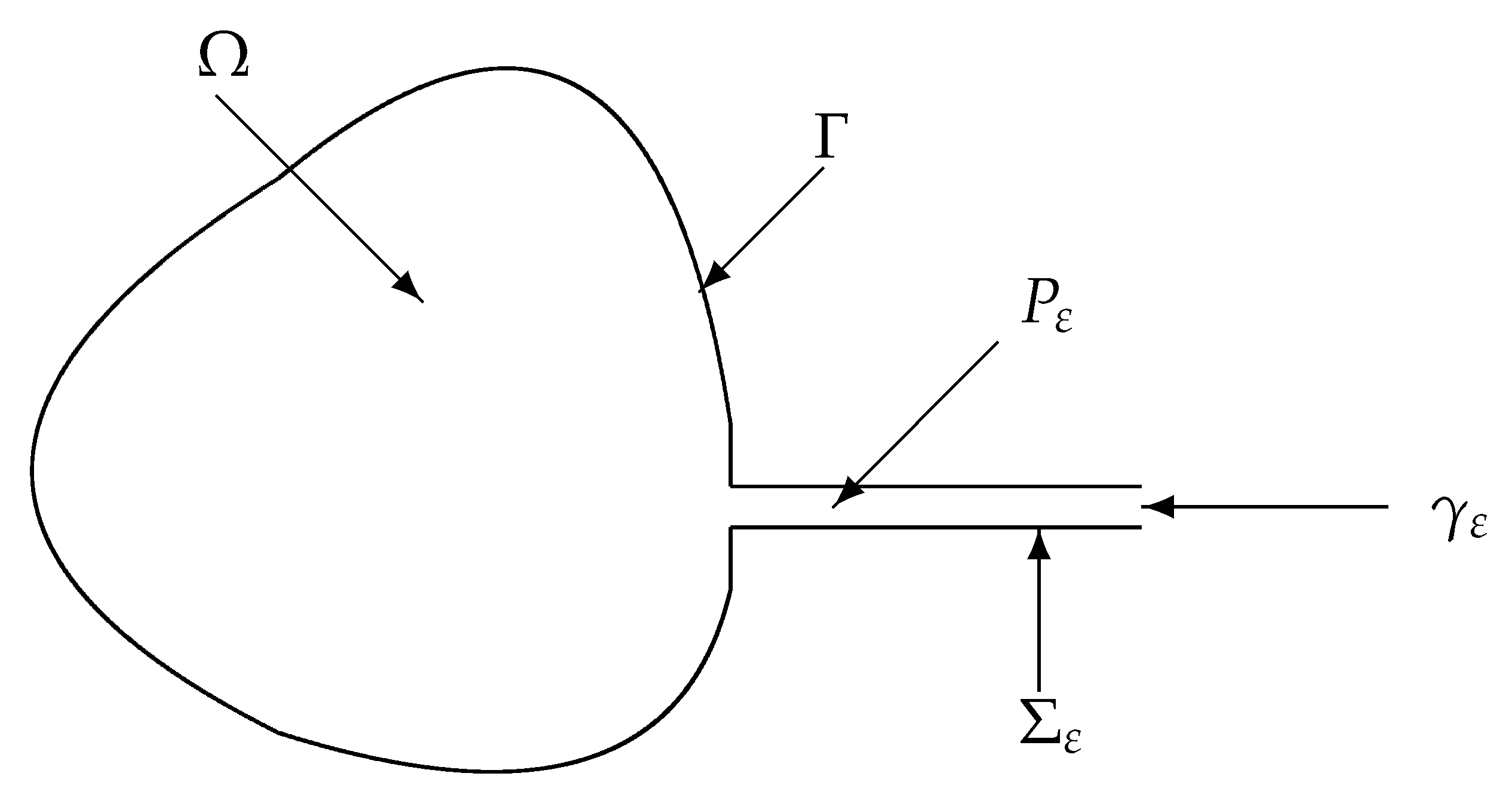
1.1. The Geometry
Let be a smooth bounded domain, such that the point . We assume that there there is a flat part of the boundary around O, i.e., there exists some such that
For smooth and convex domain contained in the unit ball , and a small parameter such that , we define the small set
and the thin pipe
The fluid domain is now defined as
We denote
Please see Figure 1.
1.2. The Equations
We denote by the velocity potential and study the Neumann problem for the Laplace equation. For the boundary condition, we first define the entering velocity as
where . We denote the total flux through the entrance of the pipe by
Next, we choose the function such that
Now, our problem reads
2. A Priori Estimates
We start with estimate.
Proposition 1.
Proof.
We test (4) with . It gives
Using the trace theorem, we obviously have
By direct integration, it is easy to prove that
with , independent from . Thus,
□
2.1. Estimate
We proceed with sharp (and essential) estimate.
Proposition 2.
Proof.
We assume, at the beginning, that .
We need an auxiliary problem:
Since the right hand-side is an function, the solution (standard elliptic regularity; see, e.g., [21]). Thus, for some . Furthermore, there exists some , independent on , such that
Testing (10) with gives
The first integral is easily estimated as above, and
For the second one, we proceed as follows:
so that
of course under the condition that . Thus, in general,
□
2.2. Estimate
The estimate in is less complicated and follows from the Ponicaré inequality:
Lemma 1.
There exists a constant , independent from ε, such that
Proof.
The classical Ponicaré inequality on yields that
with depending only on . Let . Then,
for all . A simple change of variables and (17) imply the claim. □
3. The Limit
Find such that
for any such that on .
It is easy to see that it has a unique solution (see, e.g., [18]).
Our main result is the following convergence theorem:
Theorem 1.
Proof.
Next, we take the function such that on . Then,
The bound for implies the existence of a subsequence (denoted by the same symbol) and function , such that (19) holds. Then, for the first integral, we have
For the last integral, we obtain
On the other hand,
We use here two estimates:
Finally,
We conclude from the above that the limit satisfies
which is exactly the very-weak formulation of the problems (20) and (21). It remains to prove that it has a unique solution (implying that the whole sequence converges, and not only a subsequence) in . However, (22) is the very weak formulation of the linear boundary value problem for the Laplace equation with non-smooth data, and it is well known that it has the unique very weak solution in (see, e.g., [18]). □
4. Example
To illustrate the obtained model, we solve the effective problems (20) and (21) with measure boundary data for rectangular domain . The problem reads
We assume, for simplicity, that h is a smooth even function defined on . Of course,
Due to the simple geometry, we can solve the problem (in the very-weak sense) using the Fourier method. We look for the solution of the form
where the coefficients are picked such that
If, in particular, we choose h as a constant
then
5. Conclusions
We rigorously derive a model for describing the potential flow of an ideal fluid through a reservoir with several pipes connected to it. The flow through the pipes is, usually, described by mono-dimensional models, while the flow through the reservoir is described by a three-dimensional model. The effective junction condition between the pipe and the reservoir is described by a Dirac delta measure concentrated in a junction point. The obtained problem has unique solution, but only in the very-weak sense, since the boundary value is not a function but a measure. The future goal is to do the same for the viscous flow using the concept of the very-weak solution for the Navier–Stokes system developed in [19].
Funding
This work was supported by the Croatian Science Foundation under the project AsAn (IP-2018-01-2735).
Institutional Review Board Statement
Not applicable.
Informed Consent Statement
Not applicable.
Data Availability Statement
Not applicable.
Conflicts of Interest
The author declares no conflict of interest.
References
- Blanc, F.; Gipouloux, O.; Panasenko, G.; Zine, A.M. Asymptotic analysis and partial asymptotic decomposition of domain for Stokes equation in tube structure. Math. Models Methods Appl. Sci. 1999, 9, 1351–1378. [Google Scholar] [CrossRef]
- Bourgeat, A.; Marušić-Paloka, E. Non-Linear Effects for flow in periodically constricted channel caused by high injection rate. Math. Models Methods Appl. Sci. 1998, 9, 1–25. [Google Scholar]
- Gipouloux, O.; Marušić-Paloka, E. Asymptotic behaviour of the incompressible Newtonian flow through thin constricted fracture. In Multiscale Problems in Science and Technology; Antonić, N., Duijin, C.J.V., Jaeger, W., Mikelixcx, A., Eds.; Springer: Berlin/Heidelberg, Germany, 2000; pp. 189–202. [Google Scholar]
- Marušić, S.; Marušić-Paloka, E. Two-scale convergence for thin domains and its applications to some lower-dimensional models in fluid mechanics. Asym. Anal. 2000, 23, 23–57. [Google Scholar]
- Marušić-Paloka, E. Fluid flow through a network of thin pipes. Comptes Rendus Acad. Sci. Paris Sér. II B 2001, 329, 103–108. [Google Scholar] [CrossRef]
- Marušić-Paloka, E. The effects of flexion and torsion for the fluid flow through a curved pipe. Appl. Math. Optim. 2001, 44, 245–272. [Google Scholar] [CrossRef]
- Marušić-Paloka, E. Rigorous justification of the Kirchhoff law for junction of thin pipes filled with viscous fluid. Asymptot. Anal. 2003, 33, 51–66. [Google Scholar]
- Marušić-Paloka, E.; Pažanin, I. Non-isothermal fluid flow through a thin pipe with cooling. Appl. Anal. 2009, 88, 495–515. [Google Scholar] [CrossRef]
- Marušić-Paloka, E.; Pažanin, I. On the effects of curved geometry on heat conduction through a distorted pipe. Nonlinear Anal. Real World Appl. 2010, 11, 4554–4564. [Google Scholar] [CrossRef]
- Marušić-Paloka, E.; Pažanin, I. Effects of boundary roughness and inertia on the fluid flow through a corrugated pipe and the formula for the Darcy–Weisbach friction coefficient. Int. J. Eng. Sci. 2020, 152, 103293. [Google Scholar] [CrossRef]
- Nazarov, S.A.; Piletskas, K.I. The Reynolds flow in a thin three-dimensional channel. Lith. Math. J. 1991, 30, 366–375. [Google Scholar] [CrossRef]
- Ciarlet, P. Plates and Junctions in Elastic Multi-Structures, An Asymptotic Analysis; Recherches en Mathématiques Apliquées; Springer: Berlin/Heidelberg, Germany, 1990; Volume 14. [Google Scholar]
- Le Dret, H. Problèmes Variationnels Dans Les Multi-Domaines; Recherches en Mathématiques Apliquées; Masson: Paris, France, 1991; Volume 19. [Google Scholar]
- Marušić-Paloka, E.; Marušić, S. Computation of the Permeability Tensor for a fluid Flow through a Periodic Net of Thin Channels. Appl. Anal. 1997, 64, 27–37. [Google Scholar] [CrossRef]
- Marušić-Paloka, E.; Pažanin, I. A note on Kirchhoff’s junction rule for power-law fluids. Zeitschrift fur Naturforschung 2015, 70, 695–702. [Google Scholar] [CrossRef]
- Marušić-Paloka, E. Mathematical modeling of junctions in fluid mechanics via two-scale convergence. J. Math. Anal. Appl. 2019, 480, 123399. [Google Scholar] [CrossRef]
- Panasenko, G. Method of asymptotic partial decomposition of domain. Math. Models Methods Appl. Sci. 1998, 8, 139–156. [Google Scholar] [CrossRef]
- Lions, J.L.; Magenes, E. Problèmes aux Limites Non-Homogèenes et Applications; Dunod: Paris, France, 1968; Volume 1. [Google Scholar]
- Marušić-Paloka, E. Solvability of the Navier-Stokes system with L2 boundary data. Appl. Math. Optim. 2000, 41, 365–375. [Google Scholar] [CrossRef]
- Kozlov, V.A.; Mazy’a, V.G.; Movchan, A.B. Asymptotic Analysis of Fields in Multi-Structures; Oxford Science Publications: Oxford, UK, 1999. [Google Scholar]
- Gilbarg, D.; Trudinger, N.S. Elliptic Partial Differential Equations of Second Order; Springer: Berlin/Heidelberg, Germany, 2001. [Google Scholar]
Figure 1.
The reservoir and the pipe .

Publisher’s Note: MDPI stays neutral with regard to jurisdictional claims in published maps and institutional affiliations. |
© 2021 by the author. Licensee MDPI, Basel, Switzerland. This article is an open access article distributed under the terms and conditions of the Creative Commons Attribution (CC BY) license (https://creativecommons.org/licenses/by/4.0/).
Share and Cite
MDPI and ACS Style
Marušić-Paloka, E. Modeling 3D–1D Junction via Very-Weak Formulation. Symmetry 2021, 13, 831. https://0-doi-org.brum.beds.ac.uk/10.3390/sym13050831
AMA Style
Marušić-Paloka E. Modeling 3D–1D Junction via Very-Weak Formulation. Symmetry. 2021; 13(5):831. https://0-doi-org.brum.beds.ac.uk/10.3390/sym13050831
Chicago/Turabian StyleMarušić-Paloka, Eduard. 2021. "Modeling 3D–1D Junction via Very-Weak Formulation" Symmetry 13, no. 5: 831. https://0-doi-org.brum.beds.ac.uk/10.3390/sym13050831
Note that from the first issue of 2016, this journal uses article numbers instead of page numbers. See further details here.