Universal Synthesizer of Mueller Matrices Based on the Symmetry Properties of the Enpolarizing Ellipsoid

Abstract

Polarimetry is today a widely used and powerful tool for nondestructive analysis of the structural and morphological properties of a great variety of material samples, including aerosols and hydrosols, among many others. For each given scattering measurement configuration, absolute Mueller polarimeters provide the most complete polarimetric information, intricately encoded in the 16 parameters of the corresponding Mueller matrix. Thus, the determination of the mathematical structure of the polarimetric information contained in a Mueller matrix constitutes a topic of great interest. In this work, besides a structural decomposition that makes explicit the role played by the diattenuation-polarizance of a general depolarizing medium, a universal synthesizer of Muller matrices is developed. This is based on the concept of an enpolarizing ellipsoid, whose symmetry features are directly linked to the way in which the polarimetric information is organized.

1. Introduction

Among the different techniques for determining the polarimetric properties of material media, absolute (or complete) Mueller polarimetry is particularly prominent because the measured Mueller matrix for each experimental configuration (transmission, reflection, scattering, angle of incidence and observation, spectral profile and spot-size of the probing light, measurement time, etc.) provides up to 16 independent parameters.

Such parameters contain complete information of the second-order properties of the medium regarding its linear polarimetric interaction with the probing electromagnetic wave, but they are affected by bilinear and quadratic constraining inequalities derived from the physical exigency that the eigenvalues of the positive semidefinite Hermitian coherency matrix C associated with a given Mueller matrix M are nonnegative.

Measured Mueller matrices provide information on the nature, structure, morphology and other properties of a huge variety of material samples [1], including scattering by particles, aerosols and hydrosols [2,3,4,5,6,7] where the symmetries play a key role [8,9,10,11]. A way to understand the physical information provided by M is to design a general algebraic or geometric synthesizer of Mueller matrices, where the way in which the overall polarimetric properties are generated arises in a natural manner.

From a geometric point of view, and, unlike what happens with the intensity normalized Stokes parameters of two-dimensional polarized light states, which can readily be represented geometrically by means of the Poincaré sphere, normalized Mueller matrices correspond to points located into a 15-dimensional quadric and therefore do not admit a simple and direct geometric representation akin to that of the Poincaré sphere. Nevertheless, it has been demonstrated that, up to a scale factor that regulates the mean intensity transmittance $m_{00}$ of the medium, any Mueller matrix can be represented by means of a pair of characteristic ellipsoids [12]. Since such ellipsoids are not totally independent, the formulation of a general synthesizer of Mueller matrices based on them cannot be performed in a simple and straightforward manner.

Furthermore, a general algebraic synthesizer of Mueller matrices has been developed [13] by using the normal form of a Mueller matrix [14,15,16,17,18,19,20] and tuning the indices of polarimetric purity $(P_1,P_2,P_3)$ [21] of the central canonical type-I and type-II depolarizers [19,20], which start with their maximal values $P_1=P_2=P_3=1$ (nondepolarizing, or pure, Mueller matrix) and decrease, in a consistent manner $(0\le P_1\le P_2\le P_3\le 1)$, so that any Mueller matrix can be constructed through this procedure. The problem of the synthesis of a general depolarizing Mueller matrix has also been studied by Cloude [22], who developed a parameterization that allows for modeling any depolarizing Mueller matrix from a pure one by considering all possible ways in which that the system can depolarize light. Both the above-mentioned methods are essentially algebraic and do not have a direct geometric representation.

As shown by us in a previous paper [23], the synthesis of Mueller matrices with zero diattenuation and polarizance (hereafter called nonenpolarizing) can easily be performed as a convex sum of r Mueller matrices whose associated coherency vectors are independent and belong to the image subspace of the coherency matrix C associated with M, with $r=\mathrm{rank}C$. Nevertheless, the general case of Mueller matrices exhibiting nonzero diattenuation or polarizance is more involved.

In this work, an alternative algebraic and geometric universal synthesizer of Mueller matrices is presented, which is mainly based on a specific serial-parallel composition procedure together with the geometric features of the enpolarizing ellipsoid defined from the diattenuation and polarizance properties of the Mueller matrix to be synthesized. The inverse problem of the arbitrary decomposition of a Mueller matrix into a convex sum of pure ones is particularized to the structured decomposition, where the enpolarizing properties are concentrated in one or two parallel components.

The approach presented allows for interpreting the physical information contained in any Mueller matrix M in terms of that of up to four simple nondepolarizing components, namely two diattenuators, whose combined enpolarizing features completely encompass those of M, and up to two additional retarders (which have a particularly simple mathematical representation by means of orthogonal matrices). The enpolarizing properties are intimately coupled to depolarizing ones and admit their geometric representation by means of the enpolarizing ellipsoid.

Many experimental samples correspond in practice to the particular case of a two-component structure, which is encoded in the corresponding enpolarizing ellipsoid without the necessity of considering additional retarding components.

To perform a general synthesizer of Mueller matrices, the ratios between the correlative components of the polarizance and diattenuation vectors appear as the starting parameters that can be tuned with the only restriction to satisfy the symmetry and geometric properties of the enpolarizing ellipsoid. Then, the remaining parameters necessary to build a generic Mueller matrix can be chosen in a simple manner.

The contents of this paper are organized as follows: Section 2 contains a summary of the numerous concepts and notations that are necessary to make the required developments in further sections, and that constitutes a brief review on the main topics of Mueller algebra; Section 3 is devoted to describe the structured decomposition applicable to any depolarizing Mueller matrix; the case of two-component Mueller matrices is dealt with in Section 4, where the concept of enpolarizing ellipsoid is introduced; the universal procedure for synthesizing Mueller matrices is described in Section 5, and Section 6 and Section 7 are dedicated to the discussion and conclusions, respectively.

2. Theoretical Background

Linear polarimetric interactions refer to the change of the state of polarization of light by the action of media and are represented mathematically by the transformation $s^{\prime }=Ms$ of the Stokes vector s of the incident light beam into the Stokes vector $s^{\prime }$ of the emerging beam, where M is the Mueller matrix. When M transforms any totally polarized state s into a totally polarized $s^{\prime }$, M is said to be pure (also nondepolarizing or Mueller-Jones matrix) and, wherever appropriate to distinguish it from the general depolarizing Mueller matrices, it is denoted as $M_J$. For many purposes, it is useful to express M (pure or not) in the partitioned form [24,25]

$$M=m_{00}\widehat{M},\widehat{M}\equiv \left(\begin{array}{cc}1& D^T\\ P& m\end{array}\right),$$

(1)

where the superscript T indicates transpose, $m_{00}$ is the mean intensity coefficient (MIC) (viz. the ratio between the emerging and incident intensities for incident unpolarized light), while D and P are the diattenuation and polarizance vectors, whose magnitudes D and P are the diattenuation and polarizance, respectively.

A measure of the closeness of M to a pure Mueller matrix is given by the degree of polarimetric purity (or depolarization index [26]) defined as

$$P_{\Delta }=\sqrt{\frac{\mathrm{tr}\left(M^{T}M\right)-m_{00}^2}{3m_{00}^2}}=\sqrt{\frac{1}{3}\left(D^2+P^2\right)+P_S^2},$$

(2)

where $P_S$ is the degree of spherical purity, defined as [27,28]

$$P_S\equiv \frac{1}{\sqrt{3}}\sqrt{{\displaystyle \sum _{k,l=1}^3{m}_{kl}^2}}.$$

(3)

$P_{\Delta }$ varies from $P_{\Delta }=0$ for a perfect depolarizer represented by $M_{\Delta 0}=\mathrm{diag}(m_{00},0,0,0)$, which exhibits maximum polarimetric randomness, up to $P_{\Delta }=1$, which is genuine of pure states. Concerning $P_S$, it is limited to $0\le P_S\le 1$, with $P_S=0$ for depolarizing media with $m=0$, and the maximum $P_S=1$ is exclusively achieved by pure retarders ($P=D=0$,$m=m^T$). Since diattenuation and polarizance have a common nature [27,28,29] it is sometimes useful to consider the degree of polarizance $P_P$ defined as

$$P_P\equiv \sqrt{\frac{P^2+D^2}{2}}.$$

(4)

Media with nonzero degree of polarizance are called enpolarizing, because they have the ability to increase the degree of polarization of certain incident polarized light beams. (recall that the concepts of diattenuation and polarizance should be interchanged when the directions of the incident and emerging light beams are interchanged [30]).

The difference between the magnitudes D and P of vectors D and P play an important role in the structured decomposition described in Section 3, so that it is useful to define the main enpolarizing vector Q of M as $Q=D$ when $D>P$ and $Q=P$ when $P>D$, so that the magnitude of Q is $Q=\max (D,P)$.

In the case of pure Mueller matrices $(P_{\Delta }=1)$, they can always be expressed as [31]

$$\begin{array}{c}{M}_J=m_{00}{\widehat{M}}_J,{\widehat{M}}_J=\left(\begin{array}{cc}1& D^T\\ m_{R}D& m_R{m}_D\end{array}\right),\\ \left[\begin{array}{c}{m}_D\equiv \left(\sin \kappa \right)I_3+\left(1-\sin \kappa \right)\widehat{D}\otimes {\widehat{D}}^T,m_R=m_R^T,\det m_R=+1,\\ \sin \kappa \equiv \sqrt{1-D^2},I_3\equiv \mathrm{diag}\left(1,1,1\right),\widehat{D}\equiv D/D.\end{array}\right]\end{array}$$

(5)

Pure Mueller matrices always satisfy $D=P$ [32]. When $m_R=I_3$, then $M_J$ is usually denoted as $M_D$ and corresponds to a normal diattenuator [33,34] (or homogeneous diattenuator [35]), while $D=0$ (i.e., zero diattenuation-polarizance and $m=m_R$) is characteristic of retarders, which are denoted as $M_R$ [30].

For any M, the Mueller matrix $M^r$ corresponding to the polarimetric interaction when the incident and emerging electromagnetic waves are interchanged is given by $M^r=X{M}^{T}X$, with $X=\mathrm{diag}\left(1,1,-1,1\right)$ [36,37]. Note that even though X is not a Mueller matrix (it does not satisfy the covariance conditions) both $M^T$ and $M^r$ are Mueller matrices insofar as M is a Mueller matrix [38,39].

Leaving aside experimental errors in measured Mueller matrices, the characteristic conditions for a real 4 × 4 matrix M to be a Mueller matrix are given by the combination of

(a)

Covariance conditions [40]: ${\lambda }_i\ge 0$, where ${\lambda }_i (i,j=0,1,2,3)$ are the eigenvalues of the associated (Hermitian) coherency matrix C(M), whose elements $c_{ij} (i,j=0,1,2,3)$ are defined as [41]

$$\begin{array}{c}{c}_{ij}=\frac{1}{4}\mathrm{tr}\left(G_i^{*}{G}_{j}M\right),\\ \left[G_0\equiv \left(\begin{array}{cccc}1& 0& 0& 0\\ 0& 1& 0& 0\\ 0& 0& 1& 0\\ 0& 0& 0& 1\end{array}\right),G_1\equiv \left(\begin{array}{cccc}0& 1& 0& 0\\ 1& 0& 0& 0\\ 0& 0& 0& i\\ 0& 0& -i& 0\end{array}\right),G_2\equiv \left(\begin{array}{cccc}0& 0& 1& 0\\ 0& 0& 0& -i\\ 1& 0& 0& 0\\ 0& i& 0& 0\end{array}\right),G_3\equiv \left(\begin{array}{cccc}0& 0& 0& 1\\ 0& 0& i& 0\\ 0& -i& 0& 0\\ 1& 0& 0& 0\end{array}\right)\right],\end{array}$$

(6)

and, conversely,

$$m_{ij}=\mathrm{tr}(G_i^{*}{G}_{j}C),$$

(7)

where * stands for complex conjugate.

(b)

Passivity condition: $m_{00}(1+Q)\le 1$, with $Q=\left|Q\right|=\max (D,P)$ [39,42].

When passivity constraints are not considered (as for instance in relative polarimetry, where M is measured up to a positive scale factor) it is common to represent all the equivalence class of Mueller matrices proportional to M by means of $\widehat{M}\equiv M/m_{00}$. Nevertheless, $\widehat{M}$ only satisfies the passivity condition in the particular case that $P=D=0$, and the less restrictive passive representative of M is the passive form $\tilde{M}$ of M given by [42]

$$\tilde{M}\equiv \frac{1}{1+Q}\left(\begin{array}{cc}1& D^T\\ P& m\end{array}\right),\left[Q\equiv \max \left(D,P\right)\right],$$

(8)

whose MIC ${\tilde{m}}_{00}\equiv 1/(1+Q)$ is the largest one compatible with passivity condition.

The structure of polarimetric purity-randomness of M is intrinsically related to the normalized eigenvalues ${\widehat{\lambda }}_i\equiv {\lambda }_i/m_{00}$ of C (taken so as to satisfy ${\widehat{\lambda }}_0\ge {\widehat{\lambda }}_1\ge {\widehat{\lambda }}_2\ge {\widehat{\lambda }}_3$), and a complete quantitative description of the polarimetric purity of the medium requires considering the three indices of polarimetric purity (IPP), defined as [21]

$$P_1\equiv {\widehat{\lambda }}_0-{\widehat{\lambda }}_1,P_2\equiv {\widehat{\lambda }}_0+{\widehat{\lambda }}_1-2{\widehat{\lambda }}_2,P_3\equiv {\widehat{\lambda }}_0+{\widehat{\lambda }}_1+{\widehat{\lambda }}_2-3{\widehat{\lambda }}_3,$$

(9)

which, together with P and D, provide complete information on the depolarizing properties of M in terms of invariant quantities under reversible transformations (i.e., dual-retarder transformation, see below) [28,43]. The IPP satisfy the nested inequalities $0\le P_1\le P_2\le P_3\le 1$, so that their values run through different physical situations from those of pure Mueller matrices $P_1=P_2=P_3=1$ $(P_{\Delta }=1)$, down to $P_1=P_2=P_3=0$ $(P_{\Delta }=0)$ for perfect depolarizers [21].

Conversely, the components of purity (CP) [27,28], namely D, P and $P_S$ contain full information on the sources of polarimetric purity (diattenuation, polarizance and spherical purity), which is complementary to that provided by the IPP. Thus, since $P_{\Delta }$ can be calculated either from the IPP or from the CP through the relations [27]

$$P_{\Delta }^2=\frac{1}{3}\left(2P_1^2+\frac{2}{3}{P}_2^2+\frac{1}{3}{P}_3^2\right)=\frac{1}{3}\left(D^2+P^2+3P_S^2\right),$$

(10)

$P_S$ can be calculated from the set of five parameters $(P_1,P_2,P_3,D,P)$ that constitute a minimum set of independent scalar descriptors fully characterizing the quantitative and qualitative depolarizing invariant properties of the medium represented by M.

The Mueller matrix M representing the serial action of a cascade of polarizing devices with Mueller matrices $M_1,M_2\dots M_n$ is given by their matrix product $M=M_n\dots M_2{M}_1$ (serial composition), while the Mueller matrix of a parallel composition of devices which exhibit respective relative cross sections $p_i$ with respect to the total area covered by the incident beam on the sample is given by the convex sum $M=\Sigma p_i{M}_i$, $\Sigma p_i=1$.

Among the serial decompositions of a Mueller matrix M, the dual-retarder transformations [43] are defined as $M_{R2}M{M}_{R1}$, $M_{R1}$ and $M_{R2}$ being the Mueller matrices of respective retarders (in general elliptical), and can be expressed as

$$M_E=M_{R2}M{M}_{R1}=\left(\begin{array}{cc}1& 0^T\\ 0& m_{R2}\end{array}\right)m_{00}\left(\begin{array}{cc}1& D^T\\ P& m\end{array}\right)\left(\begin{array}{cc}1& 0^T\\ 0& m_{R1}\end{array}\right)=m_{00}\left(\begin{array}{cc}1& D^T{m}_{R1}\\ m_{R2}P& m_{R2}m{m}_{R1}\end{array}\right),$$

(11)

Dual-retarder transformations are called reversible because, unlike what happens with serial transformations including enpolarizing media, they do not involve either loss of intensity (which can never be recovered by the action of natural passive media), or reduction of the degree of polarization (which cannot be recovered by the action of nonenpolarizing media).

Matrices $M_E$ obtained through dual-retarder transformations of M are called invariant-equivalent to M because the depolarizing and enpolarizing properties of M are invariant under such transformations.

Consider now the following modified singular value decomposition of the 3 × 3 submatrix m, of M

$$\begin{array}{c}m=m_{RO}{m}_A{m}_{RI},\\ \left[m_A\equiv \mathrm{diag}\left(a_1,a_2,\epsilon a_3\right),a_1\ge a_2\ge a_3\ge 0,\epsilon \equiv \left(\det m\right)/\left|\det m\right|\right],\end{array}$$

(12)

where $(a_1,a_2,a_3)$ are the singular values of m, taken in decreasing order, so that the so-called arrow decomposition of M is defined as [27,29]

$$\begin{array}{c}M=M_{RO}{M}_A{M}_{RI},\\ M_A\equiv m_{00}\left(\begin{array}{cc}1& D_A^T\\ P_A& m_A\end{array}\right)=M_{RO}^{T}M{M}_{RI}^T=m_{00}\left(\begin{array}{cc}1& D^T{m}_{RI}^T\\ m_{RO}^{T}P& m_{RO}^{T}m{m}_{RI}^T\end{array}\right),\\ \left[m_A\equiv \mathrm{diag}\left(a_1,a_2,\epsilon a_3\right),M_{RI}\equiv \left(\begin{array}{cc}1& 0^T\\ 0& m_{RI}\end{array}\right),M_{RO}\equiv \left(\begin{array}{cc}1& 0^T\\ 0& m_{RO}\end{array}\right)\right],\end{array}$$

(13)

where the Mueller matrix $M_A$ is the so-called arrow form of M [29]. From its very definition, $M_A$ has six zero elements (namely the off-diagonal elements of $m_A$) and its main virtue among other dual-retarder transformations, is that it is free of retardance information, which is fully contained in the entrance and exit retarders represented by $M_{RI}$ and $M_{RO}$ respectively [28]. Therefore, $M_A$ contains all invariant information on diattenuation, polarizance and depolarizing properties in a particularly simple and condensed manner, and the following ten independent physical quantities are invariant under the transformation from M to $M_A$ [43]

$$m_{00},P,D,a_1,a_2,a_3,P_1,P_2,P^{T}mD,\det M,$$

(14)

or, equivalently, the set of six independent physical invariants $(m_{00},D,P,P_1,P_2,P_3)$, together with the two pairs of orientation angles $({\phi }_{DA},{\chi }_{DA})$ and $({\phi }_{PA},{\chi }_{PA})$ of the diattenuation and polarizance vectors, $D_A$ and $P_A$, of $M_A$, respectively. The diattenuation and polarizance vectors of M are recovered from those of $M_A$ through the respective rotations (in the Poincaré sphere representation) $D=m_{RI}^T{D}_A$ and $P=m_{RO}{P}_A$, which are directly determined from the entrance and exit retarders $M_{RI}$ and $M_{RO}$ of M.

Obviously, other important invariant parameters like P_P, P_S and P_Δ can be derived from the above-mentioned sets. In particular, the degree of spherical purity is just determined by the singular values of m, $P_S(M)=P_S(M_A)=\sqrt{(a_1^2+a_2^2+a_3^2)/3}$.

In the special case where $P=D=0$, the arrow form of M corresponds to an intrinsic depolarizer (or diagonal depolarizer) $M_A=m_{00}\mathrm{diag}(1,a_1,a_2,\epsilon a_3)$, which is free from both enpolarizing (dichroism) and retarding (birefringence) anisotropies [43].

Regarding parallel decompositions of M into pure components, the most general formulation is given by the so-called arbitrary decomposition [1,44]

$$\begin{array}{c}M={\displaystyle \sum _{i=1}^r{k}_i{M}_{Ji}}={\displaystyle \sum _{i=1}^r{k}_i{m}_{00i}{\widehat{M}}_{Ji}},\\ \left[r=\mathrm{rank}C\left(M\right),k_i=\frac{1}{m_{00i}\left({\widehat{w}}_i^{†}{C}^{-}{\widehat{w}}_i\right)},{\displaystyle \sum _{i=1}^r{k}_i}=1\right],\end{array}$$

(15)

where ${\widehat{w}}_i$ $(i=1,\dots ,r)$ is an arbitrary set of 4-dimensional independent complex unit vectors belonging to the image subspace of $C(M)$ and $C^{-}$ is the pseudoinverse of C defined as $C^{-}=U{D}^{-}{U}^{†}$, $D^{-}$ being the diagonal matrix whose r first diagonal elements are $1/{\lambda }_1,1/{\lambda }_2,\dots ,1/{\lambda }_r$ (i.e., the inverses of the nonzero eigenvalues of C) and the last $4-r$ elements are zero.

Note that the rank r of $C(M)$ is just the number of pure components of the arbitrary decomposition of M. When $r=1$ (i.e., $P_{\Delta }=1$) a single coherency vector $\widehat{w}$ determines the corresponding pure Mueller matrix $M_J$ as well as its associated pure coherency matrix $C_J=m_{00}(\widehat{w}\otimes {\widehat{w}}^{†})$ (where ⊗ indicates the Kronecker product and the dagger stands for conjugate transpose). The expressions for the elements $m_{ij}$ of $M_J$ in terms of the associated coherency vector $w=\sqrt{m_{00}}\widehat{w}$ are given by [41]

$$m_{ij}=m_{00}{\widehat{w}}^{†}(G_i^{*}{G}_j)\widehat{w}.$$

(16)

Conversely, the elements $w_k$ $(k=0,1,2,3)$ can be expressed as follows in terms of the associated pure Mueller matrix $M_J$ [41]

$$w_k=e^{i\varphi }\frac{\sqrt{\mathrm{tr}{M}_J}}{2}\frac{\mathrm{tr}\left(G_k^{*}{G}_k{M}_J\right)}{\mathrm{tr}\left(G_k{M}_J\right)},$$

(17)

where φ is an arbitrary phase without physical significance.

The coherency vectors associated with retarders will be used in further analyses and have the general form [41]

$${\widehat{w}}_R=e^{i\gamma }\left(\begin{array}{c}i\cos \Delta /2\\ \cos 2\alpha \sin \Delta /2\\ \sin 2\alpha \sin \Delta /2\cos \delta \\ \sin 2\alpha \sin \Delta /2\sin \delta \end{array}\right),$$

(18)

where γ is an arbitrary phase without physical significance.

3. Structured Decomposition of a Mueller Matrix

It has been demonstrated [23,42] that, among the infinite possible arbitrary decompositions of any given Mueller matrix M, it is always possible to perform the structured decomposition described below, which has two alternative forms depending on whether the diattenuation equals the polarizance or not, and can be written as follows in terms of the passive form $\tilde{M}$ of M.

(a)

P = D

$$\tilde{M}=k_1{\tilde{M}}_{J1}+{\displaystyle \sum _{i=2}^r{k}_i{M}_{Ri}}.$$

(19)

(b)

P ≠ D

$$\tilde{M}=k_1{\tilde{M}}_{J1}+k_2{\tilde{M}}_{J2}+{\displaystyle \sum _{i=3}^r{k}_i{M}_{Ri}}.$$

(20)

where ${\tilde{M}}_{J1}$ and ${\tilde{M}}_{J2}$ represent passive forms of respective pure Mueller matrices with nonzero diattenuation, while $M_{Ri}$ represent retarders (hence, pure media with zero diattenuation-polarizance).

In case (a), all enpolarizing properties are located in ${\tilde{M}}_{J1}$, whose diattenuation and polarizance vectors are proportional to those of $\tilde{M}$, respectively, and the remaining $r-1$ pure components $M_{Ri}$ are retarders. In case (b), the components ${\tilde{M}}_{J1}$ and ${\tilde{M}}_{J2}$ have nonzero diattenuation, with $Q({\tilde{M}}_{J1})\uparrow \uparrow Q({\tilde{M}}_{J2})$, (the double vertical bar means that vectors on both sides are parallel, with the same direction); while the remaining $r-2$ pure components $M_{Ri}$ are retarders.

To describe the procedure to apply the structured decomposition, let us first consider depolarizing Mueller matrices satisfying $D=P$, for which the structured decomposition of M takes the form shown in Equation (19) and can be performed through the following steps:

(1)

Take vectors D and P of M as well as any proper orthogonal matrix $m_R$ satisfying $P=m_{R}D$; then ${\tilde{M}}_{J1}$ is built as (see Equation (5))

$${\tilde{M}}_{J1}=\frac{1}{1+D}\left(\begin{array}{cc}1& D^T\\ m_{R}D& m_R{m}_D\end{array}\right),\left[m_D\equiv \sqrt{1-D^2}{I}_3+\left(1-\sqrt{1-D^2}\right)\widehat{D}\otimes {\widehat{D}}^T\right],$$

(21)

(2)

By means of Equation (17), calculate the coherency vector ${\tilde{w}}_{J1}$ associated with ${\tilde{M}}_{J1}$

(3)

Calculate $r=\mathrm{rank}C(M)$ and take $r-1$ arbitrary independent unit coherency vectors of the form

$${\widehat{w}}_{Ri}=\left(\begin{array}{c}i\cos {\Delta }_i/2\\ \cos 2{\alpha }_i\sin {\Delta }_i/2\\ \sin 2{\alpha }_i\sin {\Delta }_i/2\cos {\delta }_i\\ \sin 2{\alpha }_i\sin {\Delta }_i/2\sin {\delta }_i\end{array}\right),\left(i=2\dots r-1\right),$$

(22)

(4)

By means of Equation (16) (whit $m_{00}=1$), calculate the Mueller matrices $M_{Ri}$ of the retarders associated with ${\widehat{w}}_{Ri}$.

(5)

Through Equation (15), calculate the coefficients $k_i$ corresponding to ${\tilde{M}}_{J1}$ and $M_{Ri}$ in the structured decomposition of $\tilde{M}$ in Equation (19).

(6)

Finally, since any passive Mueller matrix M can be expressed as $M=p\tilde{M}$ with $p\le 1$, the structured decomposition of M is obtained as

$$M=p\tilde{M}=k_1\left(p{\tilde{M}}_{J1}\right)+{\displaystyle \sum _{i=2}^r{k}_i\left(p{M}_{Ri}\right)}.$$

(23)

The application of the structured decomposition of M to the more general case where $D\ne P$ requires a more involved analysis whose steps are the following:

(1)

Take D and P of M and determine the main enpolarizing vector $Q(M)$ and its magnitude $Q=\max (D,P)$, so that $Q=D$ if $D>P$, and $Q=P$ if $P>D$.

(2)

Calculate the passive form $\tilde{M}$ of M as $\tilde{M}={\tilde{m}}_{00}\widehat{M}$, with ${\tilde{m}}_{00}=1/(1+Q)$, so that $M=p\tilde{M}$ with $p=m_{00}(1+Q)\le 1$.

(3a)

If $r=4$, take an arbitrary pair of mutually independent coherency vectors, ${\widehat{w}}_{R3}$ and ${\widehat{w}}_{R4}$, of the form (18) and calculate their associated Mueller matrices of the retarders $M_{R3}$ and $M_{R4}$; calculate their weights, $k_3$ and $k_4$, in the structured decomposition (20) of $\tilde{M}$ by means of Equation (15), and perform the polarimetric subtraction [45] $(\tilde{M}-k_3{M}_{R3}-k_4{M}_{R4})/(1-k_3-k_4)\equiv {\tilde{M}}_2$; go to step 4.

(3b)

If $r=3$, take an arbitrary coherency vector ${\widehat{w}}_{R3}$ of the form (18) belonging to the image subspace of $C(M)$ and calculate its associated Mueller matrix $M_{R3}$ (retarder); calculate the weight $k_3$ of $M_{R3}$ in the structured decomposition (20) of $\tilde{M}$ by means of Equation (15), and then perform the polarimetric subtraction $(\tilde{M}-k_3{M}_{R3})/(1-k_3)\equiv {\tilde{M}}_2$; go to step 4.

(3c)

If $r=2$, set $\tilde{M}\equiv {\tilde{M}}_2$ and go to step 4.

(4)

Calculate the enpolarizing components ${\tilde{M}}_{J1}$ and ${\tilde{M}}_{J2}$ of ${\tilde{M}}_2$ as well as their respective weights, ${k^{\prime }}_1$ and ${k^{\prime }}_2$ through the procedure described in ([42], Section 9). Such procedure consists of the following steps:

(4.1)

Apply a dual-retarder transformation $M_{R2}{\tilde{M}}_2{M}_{R1}\equiv {\tilde{M}}_{T2}$ that converts ${\tilde{M}}_2$ to a tridiagonal one ${\tilde{M}}_{T2}$.

(4.2)

Raise the equations obtained from $C({\tilde{M}}_{T2}){w^{\prime }}_{J2}=v\equiv {(v_1,v_2,v_3,v_4)}^T$, where the coherency vector ${w^{\prime }}_{J2}$ is set with the form ${w^{\prime }}_{J2}=\left(c{a}_1+i{a}_2,a_1+ic{a}_2,a_3+ic{a}_4,a_3-ic{a}_3\right)$, c and $a_i$ being real parameters whose values are taken in accordance with the four corresponding parametric equations $0=\mathrm{Re}{v}_1-c\mathrm{Re}{v}_2$, $0=c\mathrm{Re}{v}_3+\mathrm{Im}{v}_4$, $0=c\mathrm{Re}{v}_4-\mathrm{Im}{v}_3$, and $0=c\mathrm{Im}{v}_1-\mathrm{Im}{v}_2$, which can be solved as indicated in [42]; this ensures that ${w^{\prime }}_{J2}$ belongs to the image subspace of $C({\tilde{M}}_{T2})$ and therefore it can be considered as the coherency vector of a physically realizable parallel component of ${\tilde{M}}_{T2}$.

(4.3)

Through Equation (16), calculate the pure Mueller matrix ${M^{\prime }}_{J2}$ associated with the obtained coherency vector ${w^{\prime }}_{J2}$ and take its passive form ${\widetilde{M^{\prime }}}_{J2}$.

(4.4)

Through Equation (15), calculate the weight ${k^{\prime }}_2$ of ${\widetilde{M^{\prime }}}_{J2}$ as a parallel component of ${\tilde{M}}_{T2}$.

(4.5)

Perform the polarimetric subtraction $({\tilde{M}}_{T2}-{k^{\prime }}_2{{\tilde{M}}^{\prime }}_{J2})/(1-{k^{\prime }}_2)\equiv {{\tilde{M}}^{\prime }}_{J1}$, so that by setting ${k^{\prime }}_1=1-{k^{\prime }}_2$, the parallel decomposition ${\tilde{M}}_{T2}={k^{\prime }}_1{{\tilde{M}}^{\prime }}_{J1}+{k^{\prime }}_2{{\tilde{M}}^{\prime }}_{J2}$ is completed.

(4.6)

Retrieve ${\tilde{M}}_2$ by means of the dual-retarder transformation ${\tilde{M}}_2=M_{R2}^T{\tilde{M}}_{T2}{M}_{R1}^T$, so that, ${\tilde{M}}_2={k^{\prime }}_1{\tilde{M}}_{J1}+{k^{\prime }}_2{\tilde{M}}_{J2}$, where ${\tilde{M}}_{J1}=M_{R2}^T{{\tilde{M}}^{\prime }}_{J1}{M}_{R1}^T$ and ${\tilde{M}}_{J2}=M_{R2}^T{{\tilde{M}}^{\prime }}_{J1}{M}_{R1}^T$.

(5)

Set $k_i\equiv \left(1-k_3-k_4\right){k^{\prime }}_i$ $(i=1,2)$

(6)

Obtain the structured decomposition of $\tilde{M}$ as

$$\tilde{M}=k_1{\tilde{M}}_{J1}+k_2{\tilde{M}}_{J2}+{\displaystyle \sum _{i=3}^r{k}_i{M}_{Ri}},$$

(24)

or, by considering any MIC $m_{00}$ of M compatible with passivity, the maximal MIC ${\tilde{m}}_{00}=1/(1+Q)$ used above may be replaced by $m_{00}<{\tilde{m}}_{00}$ and the parallel decomposition of M can be performed as

$$M=k_1\left(p{\tilde{M}}_{J1}\right)+k_2\left(p{\tilde{M}}_{J2}\right)+{\displaystyle \sum _{i=3}^r{k}_i\left(p{M}_{Ri}\right),}\left[p\equiv m_{00}/{\tilde{m}}_{00}\right].$$

(25)

Besides the enpolarizing properties are concentrated in one or two components, a peculiarity of the structured decomposition is that when $D>P$ ($D<P$) the diattenuation (polarizance) vectors of M, ${M^{\prime }}_{J1}$ and ${M^{\prime }}_{J2}$ are parallel with the same direction [42]. It should be noted that the structured decomposition is not unique, but corresponds to a family of solutions.

4. General Structure of a Two-Component Mueller Matrix. The Enpolarizing Ellipsoid

The interest of studying two-component Mueller matrices is twofold; firstly, many experimental samples correspond in practice to this category [46], and, conversely, a two-component enpolarizing equivalent constituent appears as the core of the structured decomposition and allows for establishing the general synthesis procedure in Section 5.

Consider the arrow form $M_A$ of a depolarizing Mueller matrix M satisfying $r=2$ [with $r=\mathrm{rank}C(M)=\mathrm{rank}C(M_A)$] and $P\ne D$. In accordance with de definition of $M_A$ in Equation (26), the following notations and conventions will be used

$$\begin{array}{c}{M}_A=m_{00}\left(\begin{array}{cc}1& D_A^T\\ P_A& m_A\end{array}\right),\left[m_A=\mathrm{diag}\left(a_1,a_2,\epsilon a_3\right),0\le a_3\le a_2\le a_1,\epsilon =\frac{\det m}{\left|\det m\right|}=\pm 1\right],\\ D_A\equiv \left(\begin{array}{c}{D}_{A1}\\ D_{A2}\\ D_{A3}\end{array}\right)\equiv D_A\left(\begin{array}{c}\cos 2{\chi }_{DA}\cos 2{\phi }_{DA}\\ \cos 2{\chi }_{DA}\sin 2{\phi }_{DA}\\ \sin 2{\chi }_{DA}\end{array}\right),P_A\equiv \left(\begin{array}{c}{P}_{A1}\\ P_{A2}\\ P_{A3}\end{array}\right)\equiv P_A\left(\begin{array}{c}\cos 2{\chi }_{PA}\cos 2{\phi }_{PA}\\ \cos 2{\chi }_{PA}\sin 2\phi P_{PA}\\ \sin 2{\chi }_{PA}\end{array}\right),\\ \left[-\pi /4\le {\chi }_{DA},{\chi }_{PA}\le \pi /4,0\le {\phi }_{DA},{\phi }_{PA}<\pi \right].\end{array}$$

(26)

For the sake of conciseness, $D_A>P_A$ is considered to be the case (otherwise, when $D_A<P_A$, the transpose matrix $M_A^T$ instead $M_A$ should be used in the subsequent developments).

Condition $r=2$ (i.e., $0\le P_1<1$ and $P_2=P_3=1$) is equivalent to state that the four third-order principal minors are zero valued [in addition to $\det C(M_A)=0$]. Furthermore, at least one second-order principal minor is necessarily nonzero. All of these conditions result in the exigency that the end point of the diattenuation vector $D_A$ should be located in the following enpolarizing ellipsoid whose semiaxes $q_i$ are defined in terms of the ratios $t_i=P_{Ai}/D_{Ai}$ $(i=1,2,3)$

$$1=\frac{D_{A1}^2}{q_1^2}+\frac{D_{A2}^2}{q_2^2}+\frac{D_{A3}^2}{q_3^2},\left[\begin{array}{l}{q}_1\equiv \sqrt{\left(1-t_2^2\right)\left(1-t_3^2\right)}/\left(1+t_1{t}_2{t}_3\right),\hfill \\ q_2\equiv \sqrt{\left(1-t_1^2\right)\left(1-t_3^2\right)}/\left(1+t_1{t}_2{t}_3\right),\hfill \\ q_3\equiv \sqrt{\left(1-t_1^2\right)\left(1-t_2^2\right)}/\left(1+t_1{t}_2{t}_3\right),\hfill \end{array}\right]$$

(27)

Where, necessarily $\left|t_i\right|<1$, while, in addition, the ordering $a_3\le a_2\le a_1$ established for the diagonal elements of $M_A$ implies that $\left|t_3\right|\le \left|t_2\right|\le \left|t_1\right|$, which in turn implies that $q_3\le q_2\le q_1$. Also, if $P_{Ai}=D_{Ai}$ for some component ‘i’, then necessarily $P_{Ai}=D_{Ai}=0$. Therefore, the arrow form $M_A$ of a Mueller matrix M with $\mathrm{rank}C(M)=2$ exhibits a peculiar and very strict hierarchy of the involved physical parameters.

The diagonal elements of $M_A$ are linked to the ratios $t_i$ as

$$a_1=\frac{t_1+t_2{t}_3}{1+t_1{t}_2{t}_3},a_2=\frac{t_2+t_1{t}_3}{1+t_1{t}_2{t}_3},a_3=\frac{t_3+t_1{t}_2}{1+t_1{t}_2{t}_3}.$$

(28)

Moreover, in addition to condition (27), for a given value of $D\equiv \left|D_A\right|=\left|D\right|$ the end point of the diattenuation vector $D_A$ is located on the sphere defined by $D^2=D_{A1}^2+D_{A2}^2+D_{A3}^2$ so that all physically realizable configurations for $D_{Ai}$ are given by the points belonging to the intersection of the indicated sphere and the enpolarizing ellipsoid (Figure 1).

Thus, for any particular set of ratios $t_i$, the semiaxes $q_i$ are determined through Equation (27) and therefore the feasible values of D are limited by $q_3\le D\le q_1$, while the azimuth and ellipticity angles ${\phi }_{DA}$ (with $0\le {\phi }_{DA}<\pi$) and ${\chi }_{DA}$ (with $\left|{\chi }_{DA}\right|\le \pi /4$) of $D_A$ are mutually linked through

$${\cos }^{2}2{\phi }_{DA}=\frac{q_1^2{q}_2^2}{q_3^2\left(q_2^2-q_1^2\right)}\left[\frac{q_3^2-D^2}{D^2{\cos }^{2}2{\chi }_{DA}}-\frac{q_3^2}{q_2^2}+1\right],$$

(29)

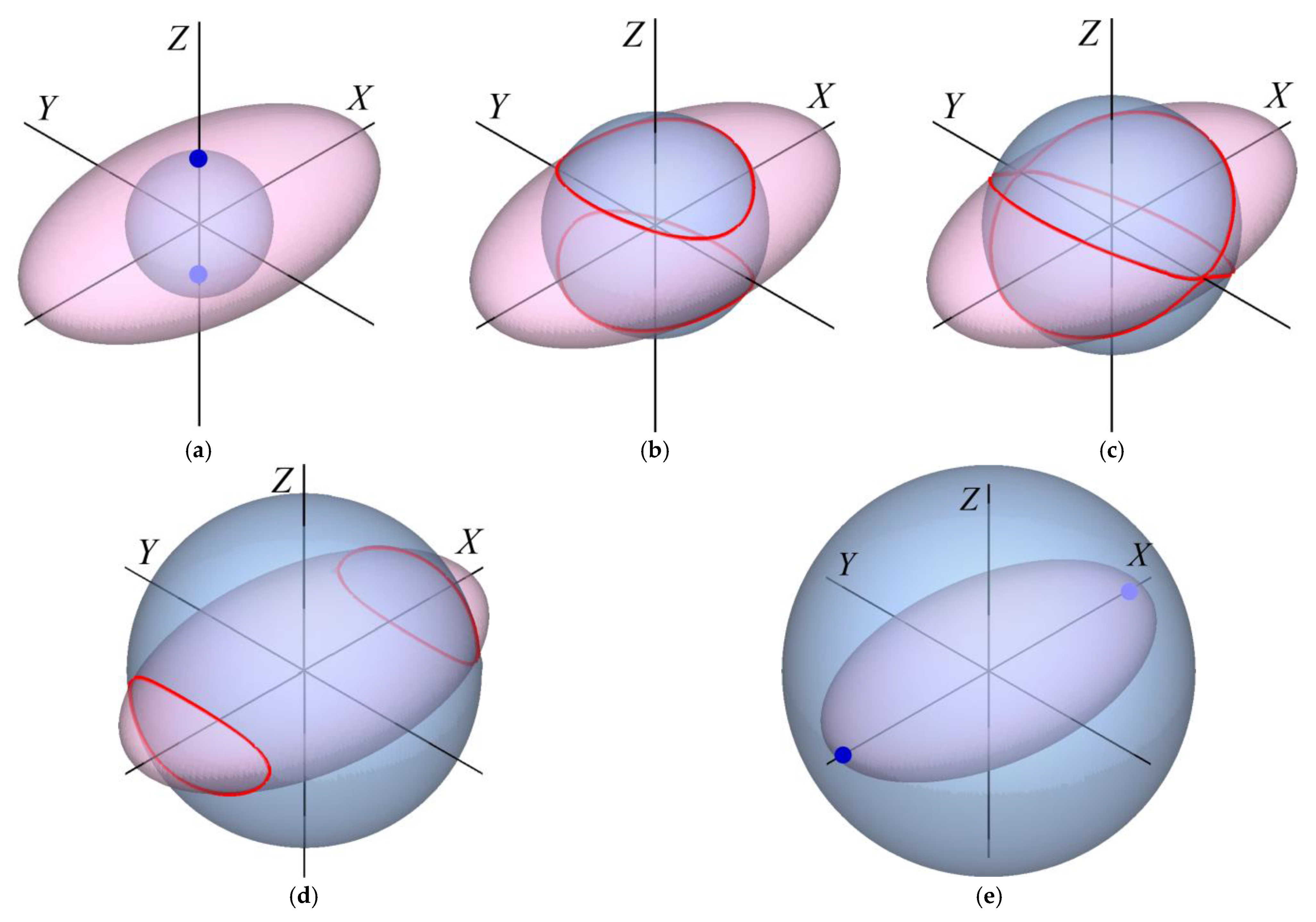
Once a set of parameters $t_i$ has been chosen, the intersection between the enpolarizing ellipsoid and the sphere of radius D varies depending on the value taken for D (with $q_3\le D\le q_1$). The smaller feasible value for D is $D=q_3$, for which the intersection is given by two single points when $q_3<q_2$, by an entire circle when $q_3=q_2$, or by the entire sphere when $q_3=q_2=q_1$. A sequence of five representative configurations is shown in Figure 1, where, in order to make a simple and clear description, the three semiaxes are taken with different values, $q_3<q_2<q_1$ (the remaining cases of ellipsoids of revolution can be analyzed straightforwardly). The symmetry axes of the enpolarizing ellipsoid determine the directions XYZ along which lie the semiaxes $q_1$, $q_2$ and $q_3$, respectively. The feasible curves start with the said pair of points corresponding to D = q₃ (such points are antipodal and located on axis Z, Figure 1a), and as D increases in the interval $q_3<D<q_2$, the intersection become pairs of closed curves on the surface of the enpolarizing ellipsoid, which are symmetrically located with respect to the plane XY (Figure 1b). When $D=q_2$, the curves become a pair of circles that intersect at points located symmetrically on both sides of axis Y (Figure 1c). As D exceeds $q_2$ and increases, the intersection is given by two closed curves symmetrically located with respect to the plane YZ (Figure 1d). In the limiting case $D=q_1$, the intersection is given by two antipodal points located in axis X (Figure 1e).

An animated representation of the intersection of the sphere of radius D and the enpolarizing ellipsoid is shown in Supplementary Materials.

5. General Procedure for the Synthesis of Mueller Matrices

From the results presented in Section 4, a systematic procedure to synthesize general Mueller matrices is the following, where the first stage is a.1, a.2, a.3 or a.4 depending on the relative values of the diattenuation and polarizance of the Mueller matrix to be synthesized:

(a.1) Construction of an enpolarizing two-component Mueller matrix with $D>P$.

(1)

Take an arbitrary set of real parameters $t_1,t_2,t_3$ satisfying $\left|t_3\right|\le \left|t_2\right|\le \left|t_1\right|<1$.

(2)

Calculate the semiaxes $q_i$ of the associated enpolarizing ellipsoid by means Equation (27).

(3)

Fix a value for D satisfying $q_3\le D\le q_1$.

(4)

Fix a value for ${\chi }_{DA}$ ($\left|{\chi }_{DA}\right|\le \pi /4$).

(5)

Determine the corresponding value for ${\phi }_{DA}$ through Equation (29), so that vector $D_A$ is fully determined by Equation (26).

(6)

Calculate the components of vector $P_A$ as $P_{Ai}=t_i{D}_{Ai}$.

(7)

Calculate $a_1,a_2,a_3$ through Equation (28).

(8)

Calculate ${\tilde{m}}_{00}=1/\left(1+D\right)$.

(9)

Build ${\tilde{M}}_{A2}$ by means of Equation (26).

(10)

Take two arbitrary Mueller matrices $M_{RI}$ and $M_{RO}$ of the entrance and exit retarders and build the two-component Mueller matrix ${\tilde{M}}_2=M_{RO}{\tilde{M}}_{A2}{M}_{RI}$.

(11)

Take an arbitrary real and positive coefficient $k$ satisfying $k\le 1$.

(12)

If $k=1$, the synthesis has been completed, resulting in the passive form of a generic two-component Mueller matrix ${\tilde{M}}_2$ with $D>P$. If $k<1$ go to (b).

(a.2) Construction of an enpolarizing two-component Mueller matrix with$P>D$.

(1)

Follow the same steps from (1) to (9) as in (a.1) and then take ${\tilde{M}}_{A2}^T$ instead of ${\tilde{M}}_{A2}$. Then, rename it as ${\tilde{M}}_{A2}$, (now ${\tilde{M}}_{A2}$ satisfies $P>D$).

(2)

Take two arbitrary Mueller matrices $M_{RI}$ and $M_{RO}$ of respective retarders and build the two-component Mueller matrix ${\tilde{M}}_2=M_{RO}{\tilde{M}}_{A2}{M}_{RI}$.

(3)

Take an arbitrary real and positive coefficient $k$ satisfying $k\le 1$.

(4)

If $k=1$, the synthesis has been completed, resulting in the passive form of a generic two-component Mueller matrix ${\tilde{M}}_2$ with $P>D$. If $k<1$ go to (b).

(a.3) Construction of an enpolarizing two-component Mueller matrix with $P=D>0$.

(1)

Build an arbitrary pure Mueller matrix ${\tilde{M}}_{J1}$ by means of Equation (5), (the diattenuation and polarizance vectors, D and P, will coincide with those of the synthesized Mueller matrix. Take ${\tilde{m}}_{00}=1/(1+D)$.

(2)

Take an arbitrary Mueller matrix of a retarder $M_{R2}$ (due to their different structures, the independence of the coherency vectors associated with ${\tilde{M}}_{J1}$ and $M_{R2}$ is directly satisfied).

(3)

Take two arbitrary real and positive coefficients $k_1$ and $k_2$ satisfying $k_1+k_2\le 1$.

(4)

Build ${\tilde{M}}_2=k_1{\tilde{M}}_{J1}+k_2{M}_{R2}$

(5)

If $k_1+k_2=1$, the synthesis has been completed, resulting in the passive form of a generic two-component Mueller matrix ${\tilde{M}}_2$ with $P=D$. If $k_1+k_2<1$, then denote $k_1+k_2\equiv k$ and go to (b).

(a.4) Construction of a non-enpolarizing two-component Mueller matrix $(P=D=0)$.

(1)

Take two arbitrary different retarders $M_{R1}$ and $M_{R2}$ (note that their associated coherency vectors are independent inasmuch as $M_{R1}\ne M_{R2}$).

(2)

Take two arbitrary real and positive coefficients $k_1$ and $k_2$ satisfying $k_1+k_2\le 1$.

(3)

Build $M_2=k_1{M}_{R1}+k_2{M}_{R2}$

(4)

If $k_1+k_2=1$, the synthesis has been completed, resulting in a generic two-component nonenpolarizing Mueller matrix. If $k_1+k_2<1$, then denote $k_1+k_2\equiv k$ and go to (b).

(b) Addition of retarders to complete the desired number of independent components.

(1)

Fix a value for r = 3,4, which determines the number of pure arbitrary components of the Mueller matrix M to be synthesized.

(2)

Take a number of r − 2 coherency vectors ${\tilde{w}}_{Ri}$ (i = 3 if r = 3, or i = 3,4, if r = 4) that are mutually independent and also independent of the eigenvectors of the coherency matrix $C({\tilde{M}}_2)$ and build the corresponding Mueller matrices of the retarders $M_{Ri}$ (a single matrix $M_{R3}$ if $r=3$, or a pair, $M_{R3}$ and $M_{R4}$, if $r=4$).

(3)

Fix the relative weights $k_3$ (if $r=3$), or $k_3$ and $k_4$ (if $r=4$) so that convexity condition $k+k_3=1$ (if $r=3$), or $k+k_3+k_4=1$ (if $r=4$) is satisfied.

(4)

The r-component passive form of the synthesized Mueller matrix is then obtained as $\tilde{M}=k{\tilde{M}}_2+k_3{M}_{R3}$ (if $r=3$) or $\tilde{M}=k{\tilde{M}}_2+k_3{M}_{R3}+k_4{M}_{R4}$ (if $r=4$).

The above procedure allows for generating the entire space of Mueller matrices in their passive forms. Obviously, the multiplication of $\tilde{M}$ by an arbitrary real positive coefficient $p<1$ produces a Mueller matrix $M=p\tilde{M}$, so that any Mueller matrix can be synthesized.

6. Discussion

The procedure developed allows for synthesizing any Mueller matrix in a systematic manner. The case where the synthesized M lacks diattenuation and polarizance (nonenpolarizing Mueller matrix) is particularly simple and does not require the use of the concept of enpolarizing ellipsoid. In general, this kind of matrices is equivalent to parallel combinations of retarders, and can also be achieved by parallel combinations of pure media whose resulting vectors D and P are zero, and therefore P_S = P_Δ, so that all the polarimetric purity comes from the closeness of M to a diagonal pure Mueller matrix.

Depolarizing Mueller matrices with $P=D>0$ are synthesized through the parallel composition of a pure medium whose Mueller matrix has the form in Equation (5) that encompasses all enpolarizing properties, and a number of up to three retarders whose coherency vectors are mutually independent. Any system with $P=D>0$ is polarimetrically indistinguishable of a system where all enpolarizing power is exhibited by a single pure component.

Depolarizing Mueller matrices with P ≠ D are synthesized through two consecutive stages.

The first stage consists of generating a two-component enpolarizing Mueller matrix with the desired arbitrary properties. The arrow form of a Mueller matrix has very peculiar properties regarding the hierarchy and structure of the enpolarizing information encoded in the components of the diattenuation and polarizance vectors, and allows for defining the associated enpolarizing ellipsoid. These features are exploited in such a manner that the mathematical conditions to obtain a matrix that satisfies the covariance and passivity criteria to be a Mueller matrix are achieved in a direct and natural manner through the use of the enpolarizing ellipsoid, whose curves of intersection with the sphere of radius $Q=\max (P,D)$ determine the feasible region of solutions compatible with the prescribed enpolarizing parameters. A general two-component Mueller matrix is then obtained through a reversible dual-retarder transformation of the previously synthesized arrow form, so that the overall diattenuating and polarizing properties of the medium as well as other invariant properties like the indices of polarimetric purity, the degree of polarimetric purity and the degree of spherical purity are preserved.

It is remarkable that two-component Mueller matrices appear in many physical situations of interest, including scattering by particles, as, for instance, in aerosols or hydrosols. Therefore, the general synthesis of two-component Mueller matrices constitutes, is by itself, one of the main results of this work.

The second stage consists of adding the required number of one or two independent retarders until the prescribed number r of components of the synthesized Mueller matrix is completed.

7. Conclusions

The problem of designing a universal synthesizer, or generator, of depolarizing Mueller matrices has been addressed by taking advantage of a number of concepts involved in polarization theory, such as the covariance and passivity conditions characterizing Mueller matrices, the serial and parallel compositions of different kinds of pure media, the coherency matrix associated with a Mueller matrix, the arrow form of a Mueller matrix, etc., together with some original approaches presented in this work such as the structured composition–decomposition of a Mueller matrix and the enpolarizing ellipsoid. In fact, the nature of the developments required involves most of the notions related to Mueller matrices algebra.

Mueller matrices represent the light–matter linear interaction regarding polarization and can be classified into pure (nondepolarizing, $P_{\Delta }=1$) and depolarizing ($P_{\Delta }<1$). Furthermore, both pure and depolarizing media may exhibit enpolarizing properties $(P_P>0)$ and the general synthesis of Mueller matrices can be performed in a specific manner through a series of different physical prescriptions that complete the entire space of Mueller matrices, namely:

Pure. As it is well-known, pure media are characterized by matrices of the form in Equation (5).

Two-component, withP = D = 0. They are generated by the parallel composition (convex sum) of pairs of arbitrary Mueller matrices of retarders, $M_{R1}$ and $M_{R2}$ (with $M_{R1}\ne M_{R2}$).

Two-component, withP = D ≠ 0. They are generated by the parallel composition of the Mueller matrices of an enpolarizing pure medium ($M_{J1}$) and a retarder ($M_{R2}$).

Two-component, withP ≠ D. They are generated by the parallel composition of two Mueller matrices ($M_{J1}$ and $M_{J2}$) of enpolarizing pure media, respectively.

Three or four-component. They are generated by the parallel composition of a two-component Mueller matrix and one or two retarders. As described in Section 5, the added retarders should be independent in the sense that coherency vectors of all components should constitute a basis (in general, nonorthogonal) in the image subspace of the coherency matrix associated with the generated Mueller matrix.

The presented synthesis procedure is directly related to that of the structured decomposition of a Mueller matrix, which is dealt with in Section 4, and provides more insight into the theory and methods for the treatment and physical interpretation of Mueller matrices.

References

- Gil, J.J. Polarimetric characterization of light and media. Eur. Phys. J. Appl. Phys. 2007, 40, 1–47. [Google Scholar] [CrossRef]
- Van de Hulst, H.C. Light Scattering from Small Particles; Wiley: New York, NY, USA, 1957. [Google Scholar]
- Bohren, C.F.; Huffman, D.R. Absorption and Scattering of Light by Small Particles; Wiley: New York, NY, USA, 1983. [Google Scholar]
- Moreno, F.; González, F. (Eds.) Light Scattering from Microstructures. In Lecture Notes in Physics; Series 534; Springer: Berlin, Germany, 1998. [Google Scholar]
- Li, C.; Kattawar, G.W.; Yang, P. Identification of aerosols by their backscattered Mueller images. Opt. Express 2006, 14, 3616–3621. [Google Scholar] [CrossRef] [PubMed]
- Gao, M.; Peng-Wang Zhai, P.-W.; Franz, B.; Hu, Y.; Knobelspiesse, K.; Werdell, P.J.; Ibrahim, A.; Xu, F.; Cairns, B. Retrieval of aerosol properties and water-leaving reflectance from multi-angular polarimetric measurements over coastal waters. Opt. Express 2018, 26, 8968–8989. [Google Scholar] [CrossRef]
- Kong, Z.; Yin, Z.; Cheng, Y.; Li, Y.; Zhang, Z.; Mei, L. Modeling and Evaluation of the Systematic Errors for the Polarization-Sensitive Imaging Lidar Technique. Remote Sens. 2020, 12, 3309. [Google Scholar] [CrossRef]
- Hu, C.-R.; Kattawar, G.W.; Parkin, M.E.; Herb, P. Symmetry theorems on the forward and backward scattering Mueller matrices for light scattering from a nonspherical dielectric scatterer. Appl. Opt. 1987, 26, 4159–4173. [Google Scholar] [CrossRef]
- Savenkov, S.N. Jones and Mueller matrices: Structure, symmetry relations and information content. In Light Scattering Reviews 4; Kokhanovsky, A.A., Ed.; Springer Praxis Books; Springer: Berlin/Heidelberg, Germany, 2009. [Google Scholar]
- Brown, A.J.; Xie, Y. Symmetry relations revealed in Mueller matrix hemispherical maps. J. Quant. Spec. Radiat. Transf. 2012, 113, 644–651. [Google Scholar] [CrossRef] [Green Version]
- Pengcheng, L.; Aziz, T.; Honghui, H.; Hui, M. Characteristic Mueller matrices for direct assessment of the breaking of symmetries. Opt. Lett. 2020, 45, 706–709. [Google Scholar]
- Ossikovski, R.; Gil, J.J.; San José, I. Poincaré sphere mapping by Mueller matrices. J. Opt. Soc. Am. A 2013, 30, 2291–2305. [Google Scholar] [CrossRef]
- Gil, J.J. From a nondepolarizing Mueller matrix to a depolarizing Mueller matrix. J. Opt. Soc. Am. A 2014, 31, 2736–2743. [Google Scholar] [CrossRef]
- Sridhar, R.; Simon, R. Normal form for Mueller matrices in polarization optics. J. Mod. Opt. 1994, 41, 1903–1915. [Google Scholar] [CrossRef]
- Bolshakov, Y.; van der Mee, C.V.M.; Ran, A.C.M.; Reichstein, B.; Rodman, L. Polar decompositions in finite dimensional indefinite scalar product spaces: Special cases and applications. In Operator Theory: Advances and Applications; Gohberg, I., Ed.; Birkhäuser Verlag: Basel, Switzerland, 1996; Volume 87, pp. 61–94. [Google Scholar]
- Bolshakov, Y.; Mee, C.V.M.; Ran, A.C.M..; Reichstein, B.; Rodman, L. Errata for: Polar decompositions in finite dimensional indefinite scalar product spaces: Special cases and applications. Integral Equ. Oper. Theory 1997, 27, 497–501. [Google Scholar] [CrossRef] [Green Version]
- Gopala Rao, A.V.; Mallesh, K.S.; Sudha, S. On the algebraic characterization of a Mueller matrix in polarization optics. I. Identifying a Mueller matrix from its N matrix. J. Mod. Opt. 1998, 45, 955–987. [Google Scholar]
- Gopala Rao, A.V.; Mallesh, K.S.; Sudha, S. On the algebraic characterization of a Mueller matrix in polarization optics. II. Necessary and sufficient conditions for Jones derived Mueller matrices. J. Mod. Opt. 1998, 45, 989–999. [Google Scholar]
- Ossikovski, R. Analysis of depolarizing Mueller matrices through a symmetric decomposition. J. Opt. Soc. Am. A 2009, 26, 1109–1118. [Google Scholar] [CrossRef]
- Ossikovski, R. Canonical forms of depolarizing Mueller matrices. J. Opt. Soc. Am. A 2010, 27, 123–130. [Google Scholar] [CrossRef]
- San José, I.; Gil, J.J. Invariant indices of polarimetric purity. Generalized indices of purity for nxn covariance matrices. Opt. Commun. 2011, 284, 38–47. [Google Scholar] [CrossRef] [Green Version]
- Cloude, S.R. Depolarization Synthesis: Understanding the optics of Mueller matrix depolarization. J. Opt. Soc. Am. A 2013, 30, 691–700. [Google Scholar] [CrossRef]
- San José, I.; Gil, J.J. Retarding parallel components of a Mueller matrix. Opt. Commun. 2020, 459, 124892. [Google Scholar] [CrossRef] [Green Version]
- Robson, B.A. The Theory of Polarization Phenomena; Clarendon Press: Oxford, UK, 1974. [Google Scholar]
- Xing, Z.-F. On the deterministic and nondeterministic Mueller matrix. J. Mod. Opt. 1992, 39, 461–484. [Google Scholar] [CrossRef]
- Gil, J.J.; Bernabéu, E. Depolarization and polarization indices of an optical system. Opt. Acta 1986, 33, 185–189. [Google Scholar] [CrossRef]
- Gil, J.J. Components of purity of a Mueller matrix. J. Opt. Soc. Am. A 2011, 28, 1578–1585. [Google Scholar] [CrossRef]
- Gil, J.J. Structure of polarimetric purity of a Mueller matrix and sources of depolarization. Opt. Commun. 2016, 368, 165–173. [Google Scholar] [CrossRef] [Green Version]
- Gil, J.J. Transmittance constraints in serial decompositions of Mueller matrices. The arrow form of a Mueller matrix. J. Opt. Soc. Am. A 2013, 30, 701–707. [Google Scholar] [CrossRef] [PubMed]
- Gil, J.J.; Ossikovski, R. Polarized Light and the Mueller Matrix Approach; CRC Press: Boca Raton, FL, USA, 2016. [Google Scholar]
- Lu, S.-Y.; Chipman, R.A. Interpretation of Mueller matrices based on polar decomposition. J. Opt. Soc. Am. A 1996, 13, 1106–1113. [Google Scholar] [CrossRef]
- Gil, J.J. Determination of Polarization Parameters in Matricial Representation. Theoretical Contribution and Development of an Automatic Measurement Device. Ph.D. Thesis, University of Zaragoza, Zaragoza, Spain, April 1983. Available online: http://zaguan.unizar.es/record/10680/files/TESIS-2013-057.pdf (accessed on 27 May 2021).
- Tudor, T.; Gheondea, A. Pauli algebraic forms of normal and nonnormal operators. J. Opt. Soc. Am. A 2007, 24, 204–210. [Google Scholar] [CrossRef] [Green Version]
- Tudor, T. Nonorthogonal polarizers: A polar analysis. Opt. Lett. 2014, 39, 1537–1540. [Google Scholar] [CrossRef]
- Lu, S.-Y.; Chipman, R.A. Homogeneous and inhomogeneous Jones matrices. J. Opt. Soc. Am. A 1994, 11, 766–773. [Google Scholar] [CrossRef]
- Sekera, Z. Scattering Matrices and Reciprocity Relationships for Various Representations of the State of Polarization. J. Opt. Soc. Am. A 1966, 56, 1732–1740. [Google Scholar] [CrossRef]
- Schönhofer, A.; Kuball, H.-G. Symmetry properties of the Mueller matrix. Chem. Phys. 1987, 115, 159–167. [Google Scholar] [CrossRef]
- Gil, J.J.; Bernabéu, E. A depolarization criterion in Mueller matrices. Opt. Acta 1985, 32, 259–261. [Google Scholar] [CrossRef]
- Gil, J.J. Characteristic properties of Mueller matrices. J. Opt. Soc. Am. A 2000, 17, 328–334. [Google Scholar] [CrossRef] [PubMed] [Green Version]
- Cloude, S.R. Group theory and polarization algebra. Optik 1986, 75, 26–36. [Google Scholar]
- San José, I.; Gil, J.J. Coherency vector formalism for polarimetric transformations. Opt. Commun. 2020, 475, 126230. [Google Scholar] [CrossRef]
- San José, I.; Gil, J.J. Characterization of passivity in Mueller matrices. J. Opt. Soc. Am. A 2000, 37, 328–334. [Google Scholar] [CrossRef] [PubMed] [Green Version]
- Gil, J.J. Invariant quantities of a Mueller matrix under rotation and retarder transformations. J. Opt. Soc. Am. A 2016, 33, 52–58. [Google Scholar] [CrossRef] [Green Version]
- Gil, J.J.; San José, I. Arbitrary decomposition of a Mueller matrix. Opt. Lett. 2019, 44, 5715–5718. [Google Scholar] [CrossRef]
- Gil, J.J.; San José, I. Polarimetric subtraction of Mueller matrices. J. Opt. Soc. Am. A 2013, 30, 1078–1088. [Google Scholar] [CrossRef]
- Ossikovski, R.; Garcia-Caurel, E.; Foldyna, M.; Gil, J.J. Application of the arbitrary decomposition to finite spot size Mueller matrix measurements. Appl. Opt. 2014, 53, 6030–6036. [Google Scholar] [CrossRef]
Figure 1.
The feasible configurations of the arrow form of a two-component of a Mueller matrix are determined by the intersection between the sphere and the enpolarizing ellipsoid, whose semiaxes , and (with ) lie in the directions XYZ, respectively: (a) , the feasible region is given by a pair of antipodal contact points located in axis Z; (b) , the feasible region is given by a pair of intersection curves symmetrically located with respect to the plane XY; (c) , the feasible region is given by a pair of crossed circles; (d) , the feasible region is given by a pair of intersection curves symmetrically located with respect to the plane YZ; (e) , the feasible region is given by a pair of antipodal contact points located in axis X.
Publisher’s Note: MDPI stays neutral with regard to jurisdictional claims in published maps and institutional affiliations. |
© 2021 by the authors. Licensee MDPI, Basel, Switzerland. This article is an open access article distributed under the terms and conditions of the Creative Commons Attribution (CC BY) license (https://creativecommons.org/licenses/by/4.0/).
Share and Cite
MDPI and ACS Style
Gil, J.J.; José, I.S. Universal Synthesizer of Mueller Matrices Based on the Symmetry Properties of the Enpolarizing Ellipsoid. Symmetry 2021, 13, 983. https://0-doi-org.brum.beds.ac.uk/10.3390/sym13060983
AMA Style
Gil JJ, José IS. Universal Synthesizer of Mueller Matrices Based on the Symmetry Properties of the Enpolarizing Ellipsoid. Symmetry. 2021; 13(6):983. https://0-doi-org.brum.beds.ac.uk/10.3390/sym13060983
Chicago/Turabian StyleGil, José J., and Ignacio San José. 2021. "Universal Synthesizer of Mueller Matrices Based on the Symmetry Properties of the Enpolarizing Ellipsoid" Symmetry 13, no. 6: 983. https://0-doi-org.brum.beds.ac.uk/10.3390/sym13060983
Note that from the first issue of 2016, this journal uses article numbers instead of page numbers. See further details here.