Application of Gamma Attenuation Technique and Artificial Intelligence to Detect Scale Thickness in Pipelines in Which Two-Phase Flows with Different Flow Regimes and Void Fractions Exist

Abstract

Scale deposits can reduce equipment efficiency in the oil and petrochemical industry. The gamma attenuation technique can be used as a non-invasive effective tool for detecting scale deposits in petroleum pipelines. The goal of this study is to propose a dual-energy gamma attenuation method with radial basis function neural network (RBFNN) to determine scale thickness in petroleum pipelines in which two-phase flows with different symmetrical flow regimes and void fractions exist. The detection system consists of a dual-energy gamma source, with Ba-133 and Cs-137 radioisotopes and two 2.54-cm × 2.54-cm sodium iodide (NaI) detectors to record photons. The first detector related to transmitted photons, and the second one to scattered photons. The transmission detector recorded two signals, which were the counts under photopeak of Ba-133 and Cs-137 with the energy of 356 keV and 662 keV, respectively. The one signal recorded in the scattering detector, total counts, was applied to RBFNN as the inputs, and scale thickness was assigned as the output.

1. Introduction

Scale deposits on the inside of surface production equipment can cause problems such as the reduction of the internal diameter of pipelines, perforation of equipment and pipelines due to corrosion, high energy consumption costs, reduced equipment life cycle, and decreased equipment efficiency in the petroleum industry. Scale problems occur in some of the oilfields around the world, caused by floods containing barium, strontium sulfate scales, and calcium. Scale deposits can hinder oil production by clogging the matrix of oil-producing formations. Moreover, scales can clog the production equipment and flowlines and hence block damage the fluid flow. The scale deposits may also occur in the down-hole pumps, heater treaters, blocking flow lines in tubes, tanks, and other production facilities. This can cause an emergency shutdown, production equipment failure, increased maintenance costs, and a reduction in overall production efficiency [1,2,3,4,5,6,7,8].

Previous studies have shown that the gamma attenuation technique can be used as an effective method for detecting mineral scales in petroleum pipelines. Oliviera et al. (2015) used a 5.08-cm × 5.08-cm NaI detector and one Cs-137 radioactive source to scan a pipe with scale deposits [7]. To scan the pipe, both source and detector were moved simultaneously with steps of 0.5 cm. For each step, a transmission gamma spectrum was captured with the NaI detector, and the measurement duration was set to 60 s. The results showed that with gamma transmission scanning, it is possible to predict the presence of scale and measure scale as well as thickness in a pipe. However, it is not possible to estimate the exact distribution of scale on the pipe wall with the technique. Teixeira et al. (2018) proposed a gamma attenuation technique to inspect scale in a pipe. The researchers implemented the Monte Carlo simulation code (MCNP) and analytical method in the study [8]. Because of the complexity of the problem, they used Artificial Neural Networks (ANN) as their analytical method. ANNs are proven solutions for complex problems and accurate predictions using less statistical training compared to other techniques used in non-linear estimations [9]. The simulated geometry contained a steel pipe that had an external diameter of 28 cm, a Cs-137 radioactive source with a divergent beam, and one 5.08-cm × 5.08-cm NaI detector. The scale considered was made of barium sulfate scale (BaSO₄) with a thickness ranging between 0.5 and 6 cm, and a step of 0.4 cm as scale layer inside the pipe. First, the optimum opening size for the collimator was established before simulating the pipe with different diameters in the range of 15–27 cm. A single-phase fluid existed inside the pipe. The research team used the internal diameter of the pipe and acquired gamma spectrum with the detector as the inputs to an artificial neural network, and the thickness of scale was the output. With this method, scale thickness was estimated with deviations below 10% for 70% of the cases. Salgado et al. (2020) utilized the MCNP6 code to investigate the possibility of using gamma attenuation technique combined with ANN for predicting scale thickness in a pipe in which a gas–oil–water three-phase flow existed [10]. The proposed simulation geometry included an iron pipe with an outer diameter of 25 cm, a Cs-137 collimated source with a divergence angle of 8.84°, and one 3.17-cm × 1.90-cm NaI detector. The study investigated an annular flow regime of three-phase flow with a constant volume fraction (30 % water, 60 % oil, and 10% gas) inside the pipe. The scale considered was BaSO₄ with thicknesses ranging from 0 to12.4 cm and a step of 0.4 cm as a scale layer. The recorded gamma energy spectrum in the detector and scale thickness were the ANN input and output, respectively. This technique estimated the scale-thickness with a relative error of 0.6%.

Existing gamma attenuation techniques for detecting scale layers in pipelines are usually considered a single-phase flow. Even in cases where a multiphase flow was considered, a simple model of a multiphase flow with a constant flow regime and volume fraction was assumed. In a real situation, however, multiphase flows with varying flow regimes and volume fractions usually exist in oil pipelines. The present study will focus on determining scale thickness in pipelines in which two-phase flows with different flow regimes and void fractions exist. To achieve this goal, a dual-energy gamma attenuation method and RBFNN was proposed.

2. Numerical Tools

2.1. Monte Carlo Simulation

The present study aims to estimate scale thickness in pipelines in which a gas–liquid two-phase flow exists. According to Beer–Lambert’s law, gamma radiation-based instruments are sensitive to the amount and type of materials that are positioned between detector and radiation source. A simple gamma radiation-based instrument comprising a detector and a radiation source that follows Beer–Lambert’s law can detect changes in one material. In the system, one known factor is the recorded signal in the detector, and one unknown factor is the change in a material amount.

The present study will consider three unknowns: scale thickness, flow patterns, and void fraction in a gas–liquid two-phase flow. In this case, a minimum of three known signals is needed. To investigate the idea of using dual energy gamma sources and two detectors for solving the aforementioned problem, MCNP-X [11] was implemented. The system includes two radioisotopes of Ba-133 and Cs-137 as the source and two NaI detectors to record the transmitted and scattered photons.

The transmission detector was positioned 5 cm away from the pipe. Moreover, the scattering detector was located at an orientation of 45^o with respect to the axial line connecting the transmission detector and the radiation source. The dual-energy source was collimated with VEC and DIR cards in MCNPX code to have a narrow beam emitting gamma radiation toward the transmission detector. In simulations, a steel pipe with a diameter and thickness of 21 cm and 0.5 cm was specified. The scale considered was a symmetric annular layer made of BaSO₄ inside the pipe wall. Scale layers with thicknesses ranging from 0 to 4 cm and a step of 0.5 cm were simulated. The liquid and gas phases in all simulation trials were investigated, and oil and air with respective densities of 0.826 g/cm³ and 0.00125 g/cm³ were considered. The simulations modeled the three typical flow patterns called stratified, homogenous, and annular flows. The percentages of the void fraction for each flow pattern ranges from 10% to 85%, with an increment of 15%. In this study, 162 simulations (3 flow patterns × 9 scale layers × 6 void fractions) were performed. It is important to mention that many studies were conducted on the measurements of multiphase flows in recent years [12,13,14,15,16,17,18,19,20,21,22,23,24,25,26,27,28,29,30,31,32,33,34].

Figure 1 shows the modeled three flow patterns with a void fraction percentage around 25% and a scale thickness of 1.5 cm.

2.2. RBFNN

In the last few years, a lot of researchers implemented ANN for different engineering applications [35,36,37,38,39,40,41,42,43,44,45,46,47,48,49,50,51,52,53,54,55,56,57,58,59,60,61,62]. An ANN employs computational units in the network to weigh and combines data from input, hidden, and output layers. There is only one hidden layer in the RBFNN and the neurons that use RBF to process the input data. The architecture of a standard RBFNN is shown in Figure 2. Input signals (x₀, x₁, x₂, …, x_n) are weighted by and connected to hidden neurons using “synaptic weights”. The neurons’ “activation” values are neuron responses. These values are considered through the activation of non-linear functions for calculating the weighted sum of their input with the addition of a bias [63]:

Equation (1) gives the weighted sum of the input and bias.

$$\mathrm{y}=\sum \left(\mathrm{weight}\ast \mathrm{input}\right)+\mathrm{bias}$$

(1)

The average distance between the data points of a vector x is calculated with RBF consisting of an N-dimensional feature and a center location v related to a template vector extracted from the training data [64]. The activation function of the hidden layer is “radbas”.

Equation (2) expresses the output from the hidden layer’s m_th node as given in [65].

$$y_m=e^{\left(-\frac{\parallel x-v_m{\parallel }^2}{2{\sigma }_m{}^2}\right)}$$

(2)

The default of σ value (spread) in MATLAB software is 1, but this value was optimized in this study. The activation function of the output layer is “purelin”.

Equation (3) gives the prediction of output from the jth node of the output layer [64,65].

$$z_j={{\displaystyle \sum }}_{m=1}^M{u}_{mj}{y}_m+b_j$$

(3)

Training the RBFNN output weights is a mathematical procedure. Provided that the centers of RBF and the scaling parameters are determined, the weights of the output layer can be calculated. The matrix of the output layer weights (W) is the result of a minimization of the error function [66]:

$$\mathrm{E} \left(\mathrm{W}\right)=\parallel \mathrm{HW}-\mathrm{Y}{\parallel }^2$$

(4)

where H and Y are the outcome of radial basis functions and desired output, respectively. The solution is given in the form W = H + Y, where H + denotes the pseudo-inverse matrix of H. The solution W is unique and can also be found by gradient descent optimization of the error function defined in Equation (4).

Despite the similarities of RBFNN with other neural network architectures such as MLPNN, RBFNN behave differently. The proposed RBF model in this paper was developed with the MATLAB 8.1.0.604 software.

The net = newrb(P, T, goal, spread, MN, DF) takes two of these arguments and returns a new radial basis network. P, T, Goal, Spread, MN, and DF are R-by-Q matrix of Q input vectors, S-by-Q matrix of Q target class vectors, Mean squared error goal, Spread of radial basis functions, Maximum number of neurons, and number of neurons to add between displays, respectively [67].

3. Application and Results

3.1. Monte Carlo Simulation

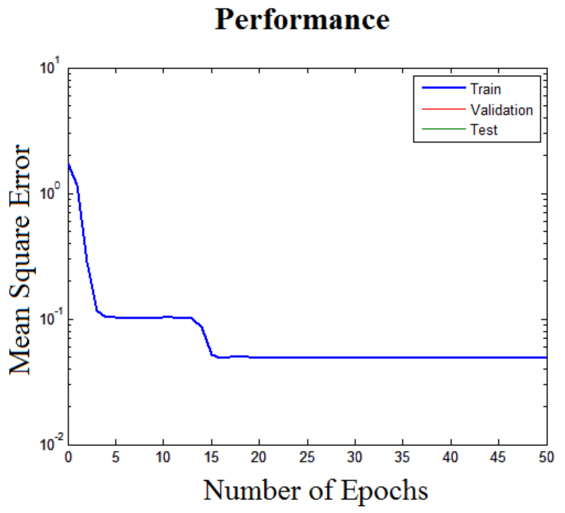
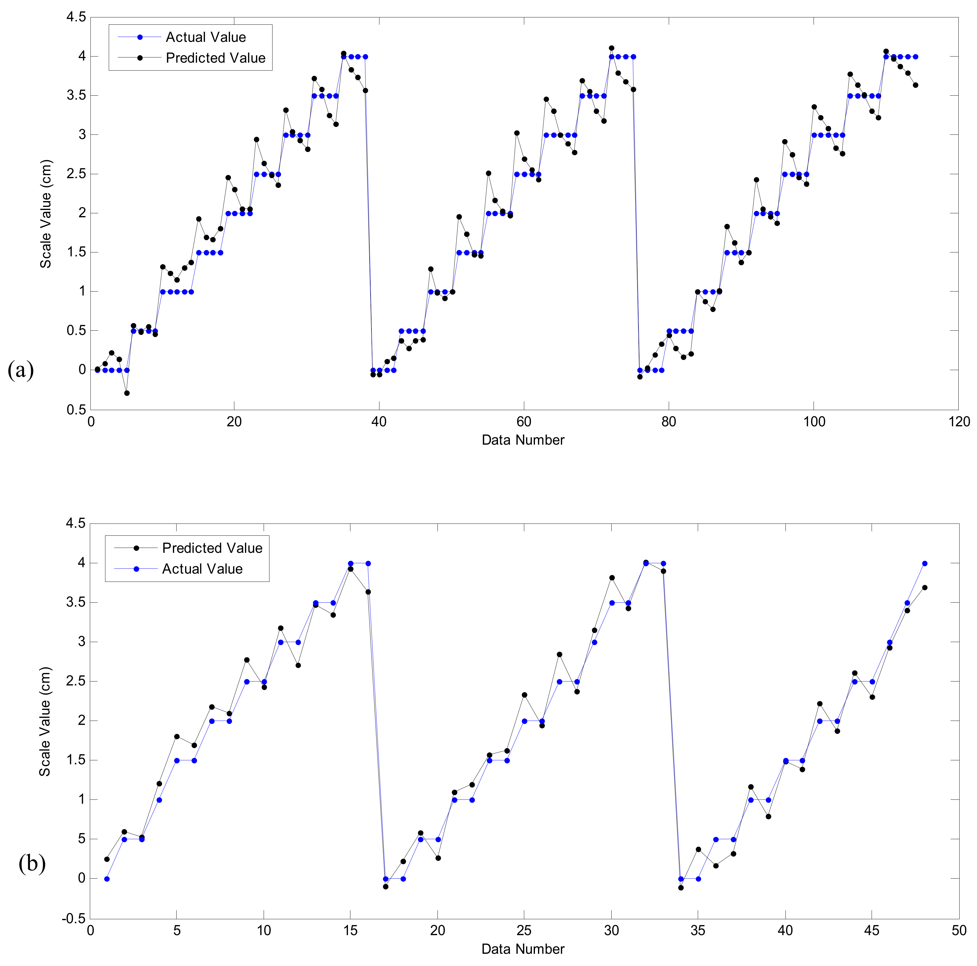
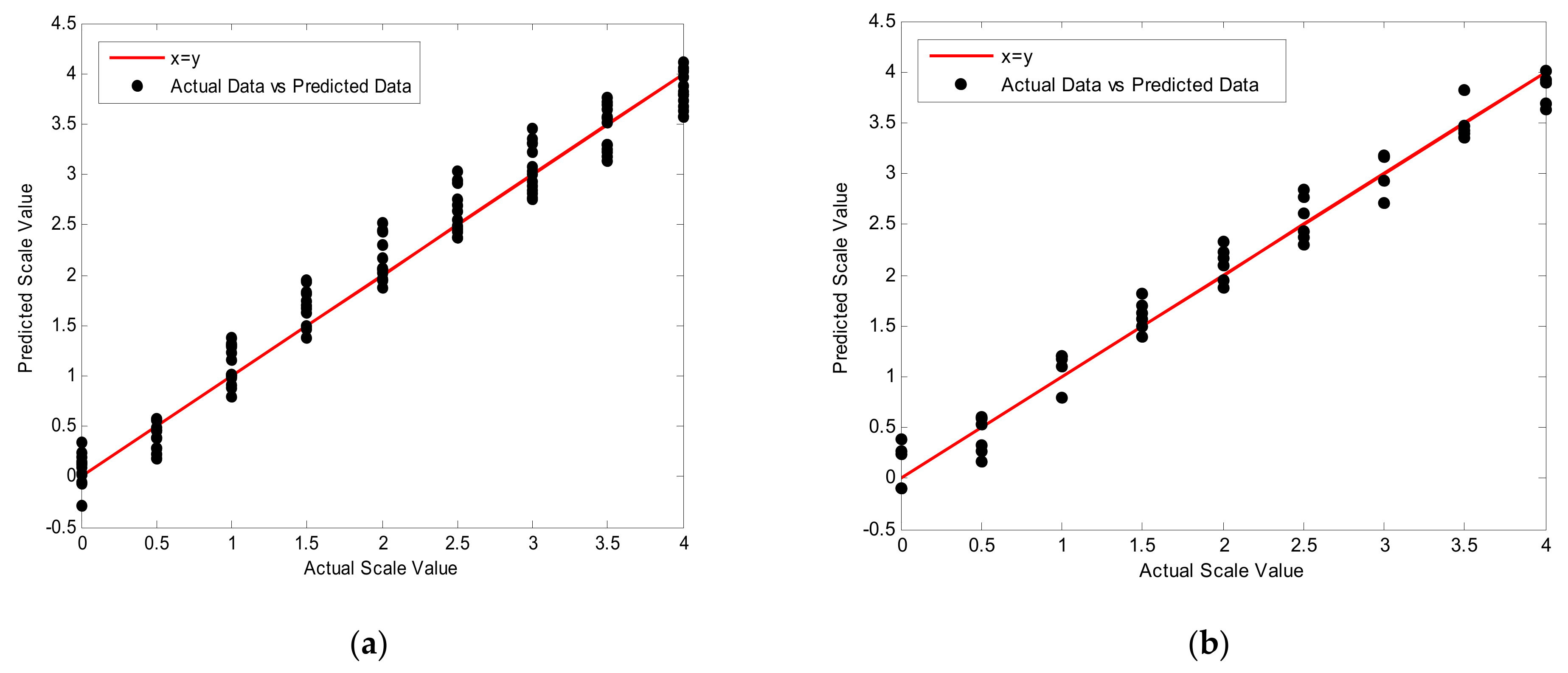
As shown in Figure 3, the transmission detector recorded two signals: the count under photopeak of Ba-133 associated with 356 keV energy and the count under photopeak of Cs-133 combined with 662 keV energy. The two signals and one signal recorded in the scattering detector, total count, were used to generate an adequate dataset for testing and training artificial neural networks.

Figure 4, Figure 5 and Figure 6 show the three recorded signals in the two detectors for different scale thicknesses and flow patterns. Recorded counts under photo peaks of Ba-133 and Cs-137 increase with decreasing the scale thickness and increasing the void fraction. In the scattering detector, a small difference in trend is observed compared with the results predicted by the transmission detector. When the scale thickness is zero, total counts slightly decrease as the void fraction increases, while for the scale thicknesses more than zero, total counts increase for the scale thicknesses greater than zero.

3.2. RBFNN

To predict the scale thickness deposited on the inner pipe wall, three different signals were extracted from both detectors and applied to the RBFNN. Gamma peak counts of Ba-133 and Cs-137 from the first transmission photons detector and total counts from the second scattered photons detector were considered as RBFNN inputs, and the scale thickness of the pipe was the RBFNN output. Figure 7 presents the flowchart of the specified RBFNN.

The best configuration of the network was obtained with the trial-and-error method.

Table 1. Configuration of proposed ANN.

ANN Type	RBFNN
Mean squared error (MSE) goal	0
Spread of radial basis functions	2
Maximum number of neurons	15
Number of neurons to add between displays	1

shows the configuration, and the schematic of the network is presented in Figure 8. In Figure 9, the error value versus the number of hidden layer neurons was plotted.

In developing the optimal RBF model, several structures were constructed and tested. The errors changed significantly until the number was increased to 15 neurons, and the error change was negligible. This behavior was shown in Figure 10, which is a performance graph. The number of neurons exceeding 15 did not improve the performance of the network but increase the complexity of the network, and hence 15 neurons were selected.

Figure 11 shows the scale thickness predicted with the proposed RBFNN (predicted values) compared with the actual values are shown for training and testing sets.

Figure 12 shows the regression plots of the actual scale thickness values and scale thicknesses predicted with the proposed RBFNN for testing and training sets.

Table 2. The errors obtained from the proposed RBFNN.

Error	Training Data	Testing Data
MAE	0.18	0.16
MRE%	0.29	0.16
RMSE	0.22	0.19
$R^2$	0.969	0.974

presents the prediction errors of the proposed RBFNN model for one output. The Mean Absolute Error (MAE), Mean Relative Error percentage (MRE%), Root Mean Square Error (RMSE) and R-squared are calculated with Equations (5) to (8).

$$MAE=\frac{1}{N}{\displaystyle \sum }_{i=1}^N\left|X_i\left(actual\right)-X_i\left(\mathrm{Pr}edicted\right)\right|$$

(5)

$$MRE\%=100\times \frac{1}{N}{\displaystyle \sum }_{i=1}^N\left|\frac{X_i\left(actual\right)-X_i\left(\mathrm{Pr}edicted\right)}{X_i\left(actual\right)}\right|$$

(6)

$$RMSE={\left[\frac{{\displaystyle {\displaystyle \sum }_{i=1}^N}{(X_i\left(actual\right)-X_i\left(\mathrm{Pr}edicted\right))}^2}{N}\right]}^{0.5}$$

(7)

$$\begin{array}{cc}{R}^2=1-\frac{{{\displaystyle \sum }}_{j=1}^N{\left(X_j\left(actual\right)-X_j\left(\mathrm{Pr}edicted\right)\right)}^2}{{{\displaystyle \sum }}_{j=1}^N{\left(X_j\left(actual\right)-\overline{X_j}\left(actual\right)\right)}^2},& \overline{X_j}\left(actual\right)=\frac{1}{N}{{\displaystyle \sum }}_{i=1}^N{X}_j\left(actual\right)\end{array}$$

(8)

where N is the number of data and ‘X_i (actual)’ and ‘X_i (Predicted)’ denote actual values and RBF predicted values, respectively.

The results presented in Figure 11 and Figure 12 and Table 2 indicate a good performance of the trained RBF neural network for estimating the scale layer thickness regardless of the type of flow regime and variations in void fraction.

It is important to mention that the coefficient of determination (R-squared) is employed as the goodness of fit index, which is defined as the proportion of variation explained by the best line model.

4. Conclusions

The present study proposed a novel approach for estimating the scale thickness in pipes in which two-phase flows with different flow patterns and void fraction exists. A dual-energy gamma attenuation method with RBFNN was used. The proposed RBFNN— with three inputs (photopeaks of Ba-133 and Cs-137 from the transmitted detector and total count from scattering detector) and one output (scale thickness)—was optimized. The optimized RBFNN consisted of 15 neurons in a hidden layer associated with a spread value of 2. The regression diagrams for both testing and training sets that showed the precision of the system were plotted. The MAE, MRE%, and RMSE of the proposed system were 0.18, 0.29, and 0.22, respectively. The results show the proposed system can be adopted in the petroleum industry for measuring scale thickness in pipes.

It is worth mentioning that the advantage of the presented system in this study is that no prior knowledge about the type of flow regime and volume fraction of multiphase components inside the pipe is required for predicting the scale thickness in case the RBF neural network is trained well. A comparative evaluation of the performance of RBFNN with other machine learning approaches is proposed for future research. Moreover, for the investigation of different pre-processing methods, different feature extraction methods, such as time domain, frequency domain, or time-frequency domain and correlation analysis, to improve the performance of the presented model are suggested.

References

1. Bahadori, A.; Zahedi, G.; Zendehboudi, S. Estimation of potential barium sulfate (barite) precipitation in oilfield brines using a simple predictive tool. Environ. Prog. Sustain. Energy 2013, 32, 860–865. [Google Scholar] [CrossRef]
2. BinMerdhah, A.B. Inhibition of barium sulfate scale at high-barium formation water. J. Pet. Sci. Eng. 2012, 90, 124–130. [Google Scholar] [CrossRef]
3. Zabihi, R.; Schaffie, M.; Nezamabadi-Pour, H.; Ranjbar, M. Artificial neural network for permeability damage prediction due to sulfate scaling. J. Pet. Sci. Eng. 2011, 78, 575–581. [Google Scholar] [CrossRef]
4. Candeias, J.P.; De Oliveira, D.F.; Dos Anjos, M.J.; Lopes, R.T. Scale analysis using X-ray microfluorescence and computed radiography. Radiat. Phys. Chem. 2014, 95, 408–411. [Google Scholar] [CrossRef]
5. Oliveira, D.F.; Santos, R.S.; Machado, A.S.; Silva, A.S.; Anjos, M.J.; Lopes, R.T. Characterization of scale deposition in oil pipelines through X-Ray Microfluorescence and X-Ray microtomography. Appl. Radiat. Isot. 2019, 151, 247–255. [Google Scholar] [CrossRef]
6. Abdul-Majid, S. Determination of wax deposition and corrosion in pipelines by neutron back diffusion collimation and neutron capture gamma rays. Appl. Radiat. Isot. 2013, 74, 102–108. [Google Scholar] [CrossRef]
7. Oliveira, D.F.; Nascimento, J.R.; Marinho, C.A.; Lopes, R.T. Gamma transmission system for detection of scale in oil exploration pipelines. Nucl. Instrum. Methods Phys. Res. Sect. A Accel. Spectrometers Detect. Assoc. Equip. 2015, 784, 616–620. [Google Scholar] [CrossRef]
8. Teixeira, T.P.; Salgado, C.M.; Dam, R.S.D.F.; Salgado, W.L. Inorganic scale thickness prediction in oil pipelines by gamma-ray attenuation and artificial neural network. Appl. Radiat. Isot. 2018, 141, 44–50. [Google Scholar] [CrossRef]
9. Tu, J.V. Advantages and disadvantages of using artificial neural networks versus logistic regression for predicting medical outcomes. J. Clin. Epidemiol. 1996, 49, 1225–1231. [Google Scholar] [CrossRef]
10. Salgado, W.L.; Dam, R.S.D.F.; Teixeira, T.P.; Conti, C.C.; Salgado, C.M. Application of artificial intelligence in scale thickness prediction on offshore petroleum using a gamma-ray densitometer. Radiat. Phys. Chem. 2020, 168, 108549. [Google Scholar] [CrossRef]
11. Pelowitz, D.B. MCNP-X TM User’s Manual, Version 2.5.0; LA-CP-05e0369; Los Alamos National Laboratory: New Mexico, NM, USA, 2005. [Google Scholar]
12. Vlasák, P.; Chára, Z.; Matoušek, V.; Konfršt, J.; Kesely, M. Experimental investigation of fine-grained settling slurry flow behaviour in inclined pipe sections. J. Hydrol. Hydromech. 2019, 67, 113–120. [Google Scholar] [CrossRef] [Green Version]
13. Roshani, M.; Phan, G.; Roshani, G.H.; Hanus, R.; Nazemi, B.; Corniani, E.; Nazemi, E. Combination of X-ray tube and GMDH neural network as a nondestructive and potential technique for measuring characteristics of gas-oil–water three phase flows. Measurement 2021, 168, 108427. [Google Scholar] [CrossRef]
14. Mosorov, V.; Zych, M.; Hanus, R.; Sankowski, D.; Saoud, A. Improvement of flow velocity measurement algorithms based on correlation function and twin plane electrical capacitance tomography. Sensors 2020, 20, 306. [Google Scholar] [CrossRef] [Green Version]
15. Salgado, C.M.; Brandão, L.E.B.; Conti, C.C.; Salgado, W.L. Density prediction for petroleum and derivatives by gamma-ray attenuation and artificial neural networks. Appl. Radiat. Isot. 2016, 116, 143–149. [Google Scholar] [CrossRef]
16. Roshani, M.; Phan, G.T.; Ali, P.J.M.; Roshani, G.H.; Hanus, R.; Duong, T.; Corniani, E.; Nazemi, E.; Kalmoun, E.M. Evaluation of flow pattern recognition and void fraction measurement in two phase flow independent of oil pipeline’s scale layer thickness. Alex. Eng. J. 2021, 60, 1955–1966. [Google Scholar] [CrossRef]
17. Sattari, M.A.; Roshani, G.H.; Hanus, R.; Nazemi, E. Applicability of time-domain feature extraction methods and artificial intelligence in two-phase flow meters based on gamma-ray absorption technique. Measurement 2021, 168, 108474. [Google Scholar] [CrossRef]
18. Roshani, G.; Hanus, R.; Khazaei, A.; Zych, M.; Nazemi, E.; Mosorov, V. Density and velocity determination for single-phase flow based on radiotracer technique and neural networks. Flow Meas. Instrum. 2018, 61, 9–14. [Google Scholar] [CrossRef]
19. Hanus, R.; Zych, M.; Mosorov, V.; Golijanek-Jędrzejczyk, A.; Jaszczur, M.; Andruszkiewicz, A. Evaluation of liquid-gas flow in pipeline using gamma-ray absorption technique and advanced signal processing. Metrol. Meas. Syst. 2021, 28, 145–159. [Google Scholar]
20. Vlasák, P.; Matoušek, V.; Chára, Z.; Krupička, J.; Konfršt, J.; Kesely, M. Concentration distribution and deposition limit of medium-coarse sand-water slurry in inclined pipe. J. Hydrol. Hydromech. 2020, 68, 83–91. [Google Scholar] [CrossRef] [Green Version]
21. Mosorov, V.; Zych, M.; Hanus, R.; Petryka, L. Modelling of dynamic experiments in MCNP5 environment. Appl. Radiat. Isot. 2016, 112, 136–140. [Google Scholar] [CrossRef]
22. El Abd, A. Intercomparison of gamma ray scattering and transmission techniques for gas volume fraction measurements in two phase pipe flow. Nucl. Instrum. Methods Phys. Res. A 2014, 735, 260–266. [Google Scholar] [CrossRef]
23. Mosorov, V.; Rybak, G.; Sankowski, D. Plug regime flow velocity measurement problem based on correlability notion and twin plane electrical capacitance tomography: Use case. Sensors 2021, 21, 2189. [Google Scholar] [CrossRef]
24. Abro, E.; Johansen, G.A. Improved void fraction determination by means of multibeam gamma-ray attenuation measurements. Flow Meas. Instrum. 1999, 10, 99–108. [Google Scholar] [CrossRef]
25. Roshani, M.; Phan, G.; Faraj, R.H.; Phan, N.-H.; Roshani, G.H.; Nazemi, B.; Corniani, E.; Nazemi, E. Proposing a gamma ra-diation based intelligent system for simultaneous analyzing and detecting type and amount of petroleum by-products. Nucl. Eng. Technol. 2021. [Google Scholar] [CrossRef]
26. Sætre, C.; Tjugum, S.A.; Johansen, G.A. Tomographic segmentation in multiphase flow measurement. Radiat. Phys. Chem. 2014, 95, 420–423. [Google Scholar] [CrossRef]
27. Salgado, W.L.; Dam, R.S.F.; Salgado, C.M. Optimization of a flow regime identification system and prediction of volume fractions in three-phase systems using gamma-rays and artificial neural network. Appl. Radiat. Isot. 2021, 169, 109552. [Google Scholar] [CrossRef]
28. Hanus, R.; Zych, M.; Kusy, M.; Jaszczur, M.; Petryka, L. Identification of liquid-gas flow regime in a pipeline using gamma-ray absorption technique and computational intelligence methods. Flow Meas. Instrum. 2018, 60, 17–23. [Google Scholar] [CrossRef]
29. Cong, T.; Chen, R.; Su, G.; Qiu, S.; Tian, W. Analysis of CHF in saturated forced convective boiling on a heated surface with impinging jets using artificial neural network and genetic algorithm. Nucl. Eng. Des. 2011, 9, 241. [Google Scholar] [CrossRef]
30. Salgado, C.M.; Pereira, C.M.N.A.; Schirru, R.; Brandao, L.E.B. Flow regime identification and volume fraction prediction in multiphase flows by means of gamma-ray attenuation and artificial neural networks. Prog. Nucl. Energy 2010, 52, 555–562. [Google Scholar] [CrossRef]
31. Barbosa, C.M.; Kenup-Hernandes, H.O.; Raitz, C.; Dam, R.S.D.F.; Salgado, W.L.; Braz, D.; Salgado, C.M. Development of a non-invasive method for monitoring variations in salt concentrations of seawater using nuclear technique and Monte Carlo simulation. Appl. Radiat. Isot. 2021, 174, 109784. [Google Scholar] [CrossRef] [PubMed]
32. Golijanek-Jędrzejczyk, A.; Mrowiec, A.; Hanus, R.; Zych, M.; Świsulski, D. Uncertainty of mass flow measurement using centric and eccentric orifice for Reynolds number in the range 10,000 ≤ Re ≤ 20,000. Measurement 2020, 160, 107851. [Google Scholar] [CrossRef]
33. Karami, A.; Roshani, G.H.; Khazaei, A.; Nazemi, E.; Fallahi, M. Investigation of different sources in order to optimize the nuclear metering system of gas–oil–water annular flows. Neural Comput. Appl. 2020, 32, 3619–3631. [Google Scholar] [CrossRef]
34. Roshani, M.; Sattari, M.A.; Ali, P.J.M.; Roshani, M.; Sattari, M.A.; Ali, P.J.M.; Roshani, G.H.; Nazemi, B.; Corniani, E.; Nazemi, E. Application of GMDH neural network technique to improve measuring precision of a simplified photon attenuation based two-phase flowmeter. Flow Meas. Instrum. 2020, 75, 101804. [Google Scholar] [CrossRef]
35. Rodriguez-Eguia, I.; Errasti, I.; Fernandez-Gamiz, U.; Blanco, J.M.; Zulueta, E.; Saenz-Aguirre, A. A parametric study of trailing edge flap implementation on three different airfoils through an artificial neuronal network. Symmetry 2020, 12, 828. [Google Scholar] [CrossRef]
36. Moradi, M.J.; Roshani, M.M.; Shabani, A.; Kioumarsi, M. Prediction of the load-bearing behavior of spsw with rectangular opening by RBF net-work. Appl. Sci. 2020, 10, 1185. [Google Scholar] [CrossRef] [Green Version]
37. Karami, A.; Veysi, F. A novel metaheuristic combinatorial algorithm to optimize the natural convection across a vertical enclosure divided by perforated flat horizontal louvers inside. Eur. Phys. J. Plus 2021, 136, 700. [Google Scholar] [CrossRef]
38. Jamshidi, M.; Lalbakhsh, A.; Talla, J.; Peroutka, Z.; Hadjilooei, F.; Lalbakhsh, P.; Jamshidi, M.; La Spada, L.; Mirmozafari, M.; Dehghani, M. Artificial intelligence and COVID-19: Deep learning approaches for diagnosis and treatment. IEEE Access 2020, 8, 109581–109595. [Google Scholar] [CrossRef]
39. Xue, H.; Yu, P.; Zhang, M.; Zhang, H.; Wang, E.; Wu, G.; Li, Y.; Zheng, X. A wet gas metering system based on the extended-throat venturi tube. Sensors 2021, 21, 2120. [Google Scholar] [CrossRef]
40. Roshani, S.; Roshani, S. Design of a high efficiency class-F power amplifier with large signal and small signal measurements. Measurement 2020, 149, 106991. [Google Scholar] [CrossRef]
41. Aghakhani, M.; Ghaderi, M.R.; Karami, A.; Derakhshan, A.A. Combined effect of TiO2 nanoparticles and input welding parameters on the weld bead penetration in submerged arc welding process using fuzzy logic. Int. J. Adv. Manuf. Technol. 2014, 70, 63–72. [Google Scholar] [CrossRef]
42. Jamshidi, M.B.; Roshani, S.; Talla, J.; Roshani, S.; Peroutka, Z. Size reduction and performance improvement of a microstrip Wilkinson power divider using a hybrid design technique. Sci. Rep. 2021, 11, 1–15. [Google Scholar] [CrossRef] [PubMed]
43. Di Nunno, F.; Alves Pereira, F.; de Marinis, G.; Di Felice, F.; Gargano, R.; Miozzi, M.; Granata, F. Deformation of air bubbles near a plunging jet using a machine learning approach. Appl. Sci. 2020, 10, 3879. [Google Scholar] [CrossRef]
44. Pirasteh, A.; Roshani, S.; Roshani, S. A modified class-F power amplifier with miniaturized harmonic control circuit. AEU Int. J. Electron. Commun. 2018, 97, 202–209. [Google Scholar] [CrossRef]
45. Lotfi, S.; Roshani, S.; Roshani, S. Design of a miniaturized planar microstrip Wilkinson power divider with harmonic cancellation. Turk. J. Electr. Eng. Comput. Sci. 2020, 28, 3126–3136. [Google Scholar] [CrossRef]
46. Jahanshahi, A.; Sabzi, H.Z.; Lau, C.; Wong, D. GPU-NEST: Characterizing energy efficiency of multi-GPU inference servers. IEEE Comput. Archit. Lett. 2020, 19, 139–142. [Google Scholar] [CrossRef]
47. Khaleghi, M.; Salimi, J.; Farhangi, V.; Moradi, M.J.; Karakouzian, M. Application of artificial neural network to predict load bearing capacity and stiffness of perforated masonry walls. CivilEng 2021, 2, 4. [Google Scholar] [CrossRef]
48. Pirasteh, A.; Roshani, S.; Roshani, S. Compact microstrip lowpass filter with ultrasharp response using a square-loaded modified T-shaped resonator. Turk. J. Electr. Eng. Comput. Sci. 2018, 26, 1736–1746. [Google Scholar] [CrossRef]
49. Arief, H.A.; Wiktorski, T.; Thomas, P.J. A survey on distributed fibre optic sensor data modelling techniques and machine learning algorithms for multiphase fluid flow estimation. Sensors 2021, 21, 2801. [Google Scholar] [CrossRef]
50. Jahanshahi, A.; Taram, M.K.; Eskandari, N. Blokus duo game on FPGA. In Proceedings of the 17th CSI International Symposium on Computer Architecture & Digital Systems (CADS 2013), October 2013; pp. 149–152. [Google Scholar]
51. Rushd, S.; Hafsa, N.; Al-Faiad, M.; Arifuzzaman, M. Modeling the settling velocity of a sphere in Newtonian and non-Newtonian fluids with machine-learning algorithms. Symmetry 2021, 13, 71. [Google Scholar] [CrossRef]
52. Moradi, M.J.; Hariri-Ardebili, M.A. Developing a library of shear walls database and the neural network based predictive meta-model. Appl. Sci. 2019, 9, 2562. [Google Scholar] [CrossRef] [Green Version]
53. Roshani, S.; Jamshidi, M.B.; Mohebi, F.; Roshani, S. Design and modeling of a compact power divider with squared resonators using artificial intelligence. Wirel. Pers. Commun. 2020. [Google Scholar] [CrossRef]
54. Jahanshahi, A. TinyCNN: A tiny modular CNN accelerator for embedded FPGA. arXiv 2019, arXiv:1911.0677. [Google Scholar]
55. Roshani, S.; Roshani, S. Two-section impedance transformer design and modeling for power amplifier applications. Appl. Comput. Electromagn. Soc. J. 2017, 32, 1042–1047. [Google Scholar]
56. Nabavi, M.; Elveny, M.; Danshina, S.D.; Behroyan, I.; Babanezhad, M. Velocity prediction of Cu/water nanofluid convective flow in a circular tube: Learning CFD data by differential evolution algorithm based fuzzy inference system (DEFIS). Int. Commun. Heat Mass Transf. 2021, 126, 105373. [Google Scholar] [CrossRef]
57. Pourjabar, S.; Choi, G.S. A high-throughput multi-mode LDPC decoder for 5G NR. arXiv 2021, arXiv:2102.13228. [Google Scholar]
58. Karami, A.; Yousefi, T.; Harsini, I.; Maleki, E.; Mahmoudinezhad, S. Neuro-fuzzy modeling of the free convection heat transfer from a wavy surface. Heat Transf. Eng. 2015, 36, 847–855. [Google Scholar] [CrossRef]
59. Darbandi, M.; Ramtin, A.R.; Sharafi, O.K. Tasks mapping in the network on a chip using an improved optimization algorithm. Int. J. Pervasive Comput. Commun. 2020, 16, 165–182. [Google Scholar] [CrossRef]
60. Roshani, G.H.; Roshani, S.; Nazemi, E.; Roshani, S. Online measuring density of oil products in annular regime of gas-liquid two phase flows. Measurement 2018, 129, 296–301. [Google Scholar] [CrossRef]
61. Arabi, M.; Dehshiri, A.M.; Shokrgozar, M. Modeling transportation supply and demand forecasting using artificial intelligence parameters (Bayesian model). J. Appl. Eng. Sci. 2018, 16, 43–49. [Google Scholar] [CrossRef] [Green Version]
62. Roshani, S.; Roshani, S. Design of a very compact and sharp bandpass diplexer with bended lines for GSM and LTE applications. AEU Int. J. Electron. Commun. 2019, 99, 354–360. [Google Scholar] [CrossRef]
63. Juliani, C.; Ellefmo, S.L. Prospectivity mapping of mineral deposits in Northern Norway using radial basis function neural networks. Minerals 2019, 9, 131. [Google Scholar] [CrossRef] [Green Version]
64. Broomhead, D.S.; Lowe, D. Multivariable functional interpolation and adaptive networks. Complex Syst. 1988, 2, 321–355. [Google Scholar]
65. Moody, J.E.; Darken, C.J. Fast learning in networks of locally-tuned processing units. Neural Comput. 1989, 1, 281–294. [Google Scholar] [CrossRef]
66. Schwenker, F.; Kestler, H.A.; Palm, G. Three learning phases for radial-basis-function networks. Neural Netw. 2001, 14, 439–458. [Google Scholar] [CrossRef]
67. MATLAB 8.0 and Statistics Toolbox 8.1; The MathWorks, Inc.: Natick, MA, USA, 2012.
Figure 1. A schematic of the modeled flows for void fraction percentage of 25% and scale-thickness of 1.5 cm. The patterns: (a) annular, (b) homogenous, and (c) stratified.
Symmetry 13 01198 g001
Figure 2. The architecture of a standard RBFNN with one input layer and hidden and output layer.
Symmetry 13 01198 g002
Figure 3. The NaI detector system and recorded signals from the detectors.
Symmetry 13 01198 g003
Figure 4. Three recorded signals in two detectors versus different void fractions and scale thicknesses for annular flow: (a) counts under photopeak of Ba-133 (b) counts under photopeak of Cs-137 (c) total counts from scattered photons detector.
Symmetry 13 01198 g004aSymmetry 13 01198 g004b
Figure 5. Three recorded signals in two detectors versus different void fractions and scale thicknesses homogenous flow: (a) counts under photopeak of Ba-133 (b) counts under photopeak of Cs-137 (c) total counts from scattered photons detector.
Symmetry 13 01198 g005aSymmetry 13 01198 g005b
Figure 6. Three recorded signals in two detectors versus different void fractions and scale thicknesses for stratified flow: (a) counts under photopeak of Ba-133, (b) counts under photopeak of Cs-137, (c) total counts from scattered photon detector.
Symmetry 13 01198 g006aSymmetry 13 01198 g006b
Figure 7. A simplified flowchart showing how the RBFNN predicted the scale thickness in the pipe with the 3 extracted signals from NaI detectors.
Symmetry 13 01198 g007
Figure 8. The Schematic of optimized RBFNN.
Symmetry 13 01198 g008
Figure 9. Error value versus the number of hidden layer neurons.
Symmetry 13 01198 g009
Figure 10. Performance graph (MSE versus number of epochs).
Symmetry 13 01198 g010
Figure 11. The Comparison of the actual and predicted values for: (a) training set (b) testing data set.
Symmetry 13 01198 g011
Figure 12. Predicted scale values versus actual data for: (a) training sets (b) testing sets.
Symmetry 13 01198 g012