A Novel Analytical View of Time-Fractional Korteweg-De Vries Equations via a New Integral Transform

Abstract

We put into practice relatively new analytical techniques, the Shehu decomposition method and the Shehu iterative transform method, for solving the nonlinear fractional coupled Korteweg-de Vries (KdV) equation. The KdV equation has been developed to represent a broad spectrum of physics behaviors of the evolution and association of nonlinear waves. Approximate-analytical solutions are presented in the form of a series with simple and straightforward components, and some aspects show an appropriate dependence on the values of the fractional-order derivatives that are, in a certain sense, symmetric. The fractional derivative is proposed in the Caputo sense. The uniqueness and convergence analysis is carried out. To comprehend the analytical procedure of both methods, three test examples are provided for the analytical results of the time-fractional KdV equation. Additionally, the efficiency of the mentioned procedures and the reduction in calculations provide broader applicability. It is also illustrated that the findings of the current methodology are in close harmony with the exact solutions. It is worth mentioning that the proposed methods are powerful and are some of the best procedures to tackle nonlinear fractional PDEs.

1. Introduction

The formulation of exact and explicit PDE solutions is essential for a good perspective on the mechanisms of diverse physical processes. Hirota and Satsuma proposed a coupled KdV framework to address the effects of two long waves with independent dispersion correlations. It was developed as an evolution equation regulating the propagation of a one-dimensional, small-amplitude, long-surface gravity wave in a shallow water channel. The non-linear coupled system of partial differential equations (PDEs) has several applications in physical systems such as fluid mechanics, aquifers, chaos, thermodynamics, plasma physics and many more. By examining a spectral $4\times 4$ equation with three possibilities, Wu et al. [1] established a unique hierarchy of nonlinear equations of evolution. Therefore, the action of the KdV solitons acknowledges the impact of the former’s existence. It is demonstrated that it determines the velocity [2,3] of the KdV subsystem. The fractional-order paired KdV equations are written as follows:

$$\begin{array}{ccc}\hfill \frac{{\partial }^{\delta }\Phi }{\partial {\overline{t}}^{\delta }}& & =-\sigma \frac{{\partial }^3\Phi }{\partial {\mathbf{x}}^3}-6\sigma \Phi \frac{\partial \Phi }{\partial \mathbf{x}}+6\Psi \frac{\partial \Psi }{\partial \mathbf{x}},\hfill \\ \hfill \frac{{\partial }^{\delta }\Psi }{\partial {\overline{t}}^{\delta }}& & =-\sigma \frac{{\partial }^3\Psi }{\partial {\mathbf{x}}^3}-3\zeta \Phi \frac{\partial \Psi }{\partial \mathbf{x}},\overline{t}>0,0<\delta \le 1,\hfill \end{array}$$

(1)

where $\sigma$ and $\zeta$ are constants and $\delta$ is the fractional order derivative of $\Phi (\mathbf{x},\overline{t})$ and $\Psi (\mathbf{x},\overline{t})$, respectively. The functions $\Phi (\mathbf{x},\overline{t})$ and $\Psi (\mathbf{x},\overline{t})$ are regarded as essential functions of space and time, vanishing for $\overline{t}$ and $\mathbf{x},$ respectively. The latter technique reduces to the conventional paired KdV equations since $\sigma =\zeta =1$ is utilized.

An exemplary equation in this scheme is the modified coupled KdV system (MCKdV). This equation is governed by the non-linear PDEs listed in [4]:

$$\begin{array}{ccc}\hfill \frac{{\partial }^{\delta }\Phi }{\partial {\overline{t}}^{\delta }}& & =\frac{1}{2}\frac{{\partial }^3\Phi }{\partial {\overline{t}}^3}-3{\Phi }^2\frac{\partial \Phi }{\partial \mathbf{x}}+\frac{3}{2}\mathsf{{\rm Y}}\frac{{\partial }^2\Psi }{\partial {\mathbf{x}}^2}+3\frac{\partial \Psi }{\partial \mathbf{x}}\frac{\partial \mathsf{{\rm Y}}}{\partial \mathbf{x}}+\frac{3}{2}\Psi \frac{{\partial }^2\mathsf{{\rm Y}}}{\partial {\mathbf{x}}^2}+3\Psi \mathsf{{\rm Y}}\frac{\partial \Phi }{\partial \mathbf{x}}+3\Phi \mathsf{{\rm Y}}\frac{\partial \Psi }{\partial \mathbf{x}}+3\Phi \Psi \frac{\partial \mathsf{{\rm Y}}}{\partial \mathbf{x}},\hfill \\ \hfill \frac{{\partial }^{\delta }\Psi }{\partial {\overline{t}}^{\delta }}& & =-\frac{{\partial }^3\Psi }{\partial {\mathbf{x}}^3}-3\frac{\partial \Phi }{\partial \mathbf{x}}\frac{\partial \Psi }{\partial \mathbf{x}}-3\Psi \frac{{\partial }^2\Phi }{\partial {\mathbf{x}}^2}-3{\Psi }^2\frac{\partial \mathsf{{\rm Y}}}{\partial \mathbf{x}}+6\Phi \Psi \frac{\partial \Phi }{\partial \mathbf{x}}+3{\Phi }^2\frac{\partial \Psi }{\partial \mathbf{x}},\hfill \\ \hfill \frac{{\partial }^{\delta }\mathsf{{\rm Y}}}{\partial {\overline{t}}^{\delta }}& & =-\frac{{\partial }^3\mathsf{{\rm Y}}}{\partial {\mathbf{x}}^3}-3\frac{\partial \Phi }{\partial \mathbf{x}}\frac{\partial \mathsf{{\rm Y}}}{\partial \mathbf{x}}-3\mathsf{{\rm Y}}\frac{{\partial }^2\Phi }{\partial {\mathbf{x}}^2}-3{\mathsf{{\rm Y}}}^2\frac{\partial \Psi }{\partial \mathbf{x}}+6\Phi \mathsf{{\rm Y}}\frac{\partial \Phi }{\partial \mathbf{x}}+3{\Phi }^2\frac{\partial \mathsf{{\rm Y}}}{\partial \mathbf{x}},\overline{t}>0,0<\delta \le 1.\hfill \end{array}$$

(2)

The modified KdV equation in its usual form is simplified by the MCKdV Equation (2), with $\Psi =\mathsf{{\rm Y}}=0.$ KdV equations are a source of non evolution equations that have a variety of applications in technology and physical sciences. The KdV equations, for example, produce ion acoustic solutions in plasma physics [5,6]. Geophysical fluid dynamics in shallow waters and deep oceans are characterized by long waves [7,8].

Numerous researchers have proposed several schemes to solve the time-fractional KdV equation using different methods, such as the Adomian decomposition method (ADM) [9], differential transform method (DTM) [10], homotopy analysis method (HAM) [11], Natural decomposition method (NDM) [12], variational iteration method [13], Elzaki projected differential transform method (EPDTM) [14], modified tanh technique (MTT) [15], new iterative method (NIM) [16], Lie symmetry analysis (LSA) [17], spectral volume method (SVM) [18,19] and so on. Analogously, similar results for (2) have been proposed by Fan [20], Cavlak and Inc [21], Inc et al. [22], Lin et al. [23], Karczewska and Szczeciński [24] and Ghoreishi et al. [25].

In recent years, the modeling of dynamical processes has progressed by incorporating notions acquired from fractional-order differential equations (FDEs). Fractional calculus resulted in the emergence of the generalization of derivatives and integrals. However, fractional calculus has a long history. Recently, it has become popular in applied sciences such as viscoelastoplastic materials, random walks, optical fibers, solid state physics, plasma physics, chaos, bifurcation, condensed matter, electromagnetic flux, image processing, virology, and biological models; memory operators called fractional derivatives are used to describe damping impacts or deterioration. Several formulations and notions of fractional derivatives were introduced by Coimbra, Davison and Essex, Riesz, Riemann–Liouville, Hadamard, Weyl, Jumarie, Grünwald–Letnikov, and Liouville–Caputo [26,27,28,29], and the characteristics of these derivatives are investigated in [30,31,32,33]. Because of their prominent features and direct physical interpretation, the implementation of the Caputo fractional derivative is gaining popularity in physics, whereas the Liouville–Caputo has a singularity in its kernel.

Maitama and Zhao [34] recently identified the Shehu transformation as an important integral transformation. The Shehu transform (ST) is a modification of the Laplace transformation. Alternately, by inserting $\omega =1$ in ST, then we recapture the Laplace transform. Complex non-linear PDEs can be converted to simpler equations via this procedure.

Despite the tremendous boost that was provided by Gorge Adomian in 1980 is known as the Adomian decomposition method (ADM). It has been successfully applied to a variety of physical models of PDEs, such as Burger’s equation, a nonlinear second-order PDE with numerous applications in applied sciences. The ADM correlated with several integral transforms, such as Laplace, modified Laplace, Mohand, Aboodh, Elzaki and many more. Recently, modified Laplace ADM [35] for solving nonlinear Volterra integral and integro-differential equations based on the Newton–Raphson formula, Discrete ADM [36] used for solving time-fractional Navier–Stokes equation, Laplace ADM [37] for finding the numerical solution of a fractional order epidemic model of a vector-born disease and hence forth.

Daftardar-Gejji and Jafari [38] proposed a new recursive approach for solving functional equations with asymptotic solutions. The novel recursive process is framed on the basis of decaying the nonlinear terms is known as the iterative Laplace transform method [39]. This process is fast and precise, and it avoids the use of an unconditioned matrix, complicated integrals, and infinite series forms. This method does not necessitate any explicit settings for the problem. Several studies have considered NITM to solve PDEs, such as the KdV Equation [16], Fornberg–Whitham equation [40], and Klein–Gordon equations [41].

Despite the significant body of work on fractional PDEs models, estimating the approximate-analytical solutions of the corresponding governing PDE is not a trivial task. In this context, we aim to develop two efficient algorithms for estimating the approximate-analytical solutions of KdV and MCKdV equations that model the dynamics of the process under investigation. The ADM and NITM are modified with the ST, and the new method is known to be the Shehu decomposition method and Shehu iterative transform method. The novel methods are applied to examining the fractional-order of the system of KDV equations. The outcome of some test examples was examined in order to demonstrate the practicality of the proposed strategy. Innovative techniques are used to derive the outcomes of the fractional-order and integral-order models. The convergence and uniqueness analysis for SDM is also presented. Using synthetic trajectories derived from the KdV and MCKdV models, we demonstrate the validity and feasibility of the suggested algorithmic approaches to deriving the approximate-analytical solutions in a simulation study. The proposed method can be used to solve other fractional orders of linear and non-linear PDEs.

2. Preliminaries

Several definitions and axiom outcomes from the literature are prerequisites in our analysis.

Definition 1

([34]). Shehu transform (ST) for a function $\Phi \left(\overline{t}\right)$ having exponential order over the set of functions is stated as

$$\begin{array}{c}\hfill \mathbb{S}=\left\{\Phi \left(\overline{t}\right)|\exists \mathcal{K},k_1,k_2>0,|\Phi \left(\overline{t}\right)|<\mathcal{K}exp(|\overline{t}|/k_j),if\overline{t}\in {(-1)}^j\times [0,\infty ),j=1,2;\left(\mathcal{K},k_1,k_2>0\right)\right\},\end{array}$$

(3)

where $\Phi \left(\overline{t}\right)$ is represented by $\mathbb{S}\left[\Phi \left(\overline{t}\right)\right]=\mathcal{S}(\xi ,\omega ),$ is described as

$$\begin{array}{c}\hfill \mathbb{S}\left[\Phi \left(\overline{t}\right)\right]=\underset{0}{\overset{\infty }{\int }}\Phi \left(\overline{t}\right)exp\left(-\frac{\xi }{\omega }\overline{t}\right)d\overline{t}=\mathcal{S}(\xi ,\omega ),\overline{t}\le 0,\omega \in [{\kappa }_1,{\kappa }_2].\end{array}$$

(4)

A useful result of the ST is stated as:

$$\begin{array}{c}\hfill \mathbb{S}\left[{\overline{t}}^{\delta }\right]=\underset{0}{\overset{\infty }{\int }}exp\left(-\frac{\xi }{\omega }\overline{t}\right){\overline{t}}^{\delta }d\overline{t}=(\delta +1){\left(\frac{\omega }{\xi }\right)}^{\delta +1}.\end{array}$$

(5)

Definition 2

([34]). The inverse ST of a mapping $\Phi \left(\overline{t}\right)$ is stated as

$$\begin{array}{c}\hfill {\mathbb{S}}^{-1}\left[{\left(\frac{\omega }{\xi }\right)}^{m\delta +1}\right]=\frac{{\overline{t}}^{m\delta }}{\Gamma (m\delta +1)},\Re \left(\delta \right)>0,andm>0.\end{array}$$

(6)

Lemma 1.

(Linearity property of ST) Let ST of ${\Phi }_1\left(\overline{t}\right)$ and ${\Phi }_2\left(\overline{t}\right)$ are $\mathcal{P}(\xi ,\omega )$ and $\mathcal{Q}(\xi ,\omega )$, respectively, [34],

$$\begin{array}{ccc}\hfill \mathbb{S}\left[{\gamma }_1{\Phi }_1\left(\overline{t}\right)+{\gamma }_2{\Phi }_2\left(\overline{t}\right)\right]& & =\mathbb{S}\left[{\gamma }_1{\Phi }_1\left(\overline{t}\right)\right]+\mathbb{S}\left[{\gamma }_2{\Phi }_2\left(\overline{t}\right)\right]\hfill \\ & & ={\gamma }_1\mathcal{P}(\xi ,\omega )+{\gamma }_2\mathcal{Q}(\xi ,\omega ),\hfill \end{array}$$

(7)

where ${\gamma }_1$ and ${\gamma }_2$ are arbitrary constants.

Lemma 2

([34]). ST of Caputo fractional derivative of order δ is stated as

$$\begin{array}{c}\hfill \mathbb{S}\left[{\mathcal{D}}_{\overline{t}}^{\delta }\Phi \left(\overline{t}\right)\right]={\left(\frac{\xi }{\omega }\right)}^{\delta }\mathbb{S}\left[\Phi (\mathbf{x},\overline{t})\right]-\sum _{\kappa =0}^{m-1}{\left(\frac{\xi }{\omega }\right)}^{\delta -\kappa -1}{\Phi }^{\left(\kappa \right)}(\mathbf{x},0),m-1\le \delta \le m,m\in \mathbb{N}.\end{array}$$

(8)

3. Configuration of the SDM

Assume the nonlinear fractional PDE:

$$\begin{array}{c}\hfill {\mathcal{D}}_{\overline{t}}^{\delta }\Phi (\mathbf{x},\overline{t})+\mathcal{L}\Phi (\mathbf{x},\overline{t})+\mathcal{N}\Phi (\mathbf{x},\overline{t})=\mathcal{F}(\mathbf{x},\overline{t}),\overline{t}>0,0<\delta \le 1\end{array}$$

(9)

subject to the condition

$$\begin{array}{c}\hfill \Phi (\mathbf{x},0)=\mathcal{G}\left(\mathbf{x}\right),\end{array}$$

(10)

where ${\mathcal{D}}_{\overline{t}}^{\delta }=\frac{{\partial }^{\delta }\Phi (\mathbf{x},\overline{t})}{\partial {\overline{t}}^{\delta }}$ denotes the fractional-order Caputo derivative operator with $0<\delta \le 1$ while $\mathcal{L}$ and $\mathcal{N}$ are linear and nonlinear terms and $\mathcal{F}(\mathbf{x},\overline{t})$ indicates the source term.

Employing the Shehu transform to (9), and we acquire

$$\begin{array}{c}\hfill \mathbb{S}\left[{\mathcal{D}}_{\overline{t}}^{\delta }\Phi (\mathbf{x},\overline{t})+\mathcal{L}\Phi (\mathbf{x},\overline{t})+\mathcal{N}\Phi (\mathbf{x},\overline{t})\right]=\mathbb{S}\left[\mathcal{F}(\mathbf{x},\overline{t})\right].\end{array}$$

Taking differentiation property of Shehu transform, we find

$$\begin{array}{ccc}\hfill & & \frac{{\xi }^{\delta }}{{\omega }^{\delta }}\mathcal{U}(\xi ,\omega )=\sum _{\kappa =0}^{m-1}{\left(\frac{\xi }{\omega }\right)}^{\delta -\kappa -1}{\Phi }^{\left(\kappa \right)}\left(0\right)+\mathbb{S}\left[\mathcal{L}\Phi (\mathbf{x},\overline{t})+\mathcal{N}\Phi (\mathbf{x},\overline{t})\right]+\mathbb{S}\left[\mathcal{F}(\mathbf{x},\overline{t})\right].\hfill \end{array}$$

(11)

Th inverse Shehu transform of (11) gives

$$\begin{array}{c}\hfill \Phi (\mathbf{x},\overline{t})={\mathbb{S}}^{-1}\left[\sum _{\kappa =0}^{m-1}{\left(\frac{\xi }{\omega }\right)}^{\delta -\kappa -1}{\Phi }^{\left(\kappa \right)}\left(0\right)+\frac{{\omega }^{\delta }}{{\xi }^{\delta }}\mathbb{S}\left[\mathcal{F}(\mathbf{x},\overline{t})\right]\right]-{\mathbb{S}}^{-1}\left[\frac{{\omega }^{\delta }}{{\xi }^{\delta }}\mathbb{S}\left[\mathcal{L}\Phi (\mathbf{x},\overline{t})+\mathcal{N}\Phi (\mathbf{x},\overline{t})\right]\right].\end{array}$$

(12)

The Shehu decomposition method solution $\Phi (\mathbf{x},\overline{t})$ is represented by the following infinite series

$$\begin{array}{c}\hfill \Phi (\mathbf{x},\overline{t})=\sum _{m=0}^{\infty }{\Phi }_m(\mathbf{x},\overline{t}).\end{array}$$

(13)

Thus, the nonlinear term $\mathcal{N}(\mathbf{x},\overline{t})$ can be evaluated by the Adomian decomposition method prescribed as

$$\begin{array}{c}\hfill \mathcal{N}\Phi (\mathbf{x},\overline{t})=\sum _{m=0}^{\infty }{\tilde{A}}_m({\Phi }_0,{\Phi }_1,...),m=0,1,...,\end{array}$$

(14)

where

$${\tilde{A}}_m({\Phi }_0,{\Phi }_1,...)=\frac{1}{m!}{\left[\frac{d^m}{d{\lambda }^m}\mathcal{N}\left(\sum _{j=0}^{\infty }{\lambda }^j{\Phi }_j\right)\right]}_{\lambda =0},m>0.$$

Substituting (13) and (14) into (12), we have

$$\begin{array}{ccc}\hfill \sum _{m=0}^{\infty }{\Phi }_m(\mathbf{x},\overline{t})& & =\mathcal{G}\left(\mathbf{x}\right)+\tilde{\mathcal{G}}\left(\mathbf{x}\right)-{\mathbb{S}}^{-1}\left[\frac{{\omega }^{\delta }}{{\xi }^{\delta }}\mathbb{S}[\mathcal{L}\Phi (\mathbf{x},\overline{t})+\sum _{m=0}^{\infty }{\tilde{A}}_m]\right].\hfill \end{array}$$

(15)

Finally, the iterative procedure for (15) is obtained as follows:

$$\begin{array}{ccc}\hfill {\Phi }_0(\mathbf{x},\overline{t})& & =\mathcal{G}\left(\mathbf{x}\right)+\tilde{\mathcal{G}}\left(\mathbf{x}\right),m=0,\hfill \\ \hfill {\Phi }_{m+1}(\mathbf{x},\overline{t})& & =-{\mathbb{S}}^{-1}\left[\frac{{\omega }^{\delta }}{{\xi }^{\delta }}\mathbb{S}\left[\mathcal{L}\left({\Phi }_m(\mathbf{x},\overline{t})\right)+\sum _{m=0}^{\infty }{\tilde{A}}_m\right]\right],m\ge 1.\hfill \end{array}$$

(16)

4. Basic Formulation of the SITM

Let us suppose the following general fractional PDE:

$$\begin{array}{c}\hfill {\mathcal{D}}_{\overline{t}}^{\delta }\Phi (\mathbf{x},\overline{t})+\mathcal{L}\Phi (\mathbf{x},\overline{t})+\mathcal{N}\Phi (\mathbf{x},\overline{t})=\mathcal{F}(\mathbf{x},\overline{t}),\overline{t}>0,m-1<\delta \le m,m\in \mathbb{N}\end{array}$$

(17)

subject to the condition

$$\begin{array}{c}\hfill {\Phi }^{\left(\kappa \right)}(\mathbf{x},0)={\mathcal{G}}_{\kappa }\left(\mathbf{x}\right),\kappa =0,1,2,...,m-1,\end{array}$$

(18)

where $\mathcal{L}$ and $\mathcal{N}$ are linear and nonlinear terms and $\mathcal{F}(\mathbf{x},\overline{t})$ indicates the source term.

Utilizing the Shehu transform to (17), we obtain

$$\begin{array}{c}\hfill \mathbb{S}\left[{\mathcal{D}}_{\overline{t}}^{\delta }\Phi (\mathbf{x},\overline{t})+\mathcal{L}\Phi (\mathbf{x},\overline{t})+\mathcal{N}\Phi (\mathbf{x},\overline{t})\right]=\mathbb{S}\left[\mathcal{F}(\mathbf{x},\overline{t})\right].\end{array}$$

Taking differentiation property of Shehu transform, we find

$$\begin{array}{ccc}\hfill & & \frac{{\xi }^{\delta }}{{\omega }^{\delta }}\mathcal{U}(\xi ,\omega )=\sum _{\kappa =0}^{m-1}{\left(\frac{\xi }{\omega }\right)}^{\delta -\kappa -1}{\Phi }^{\left(\kappa \right)}\left(0\right)+\mathbb{S}\left[\mathcal{L}\Phi (\mathbf{x},\overline{t})+\mathcal{N}\Phi (\mathbf{x},\overline{t})\right]+\mathbb{S}\left[\mathcal{F}(\mathbf{x},\overline{t})\right].\hfill \end{array}$$

(19)

Th inverse Shehu transform of (19) gives

$$\begin{array}{c}\hfill \Phi (\mathbf{x},\overline{t})={\mathbb{S}}^{-1}\left[\sum _{\kappa =0}^{m-1}{\left(\frac{\xi }{\omega }\right)}^{\delta -\kappa -1}{\Phi }^{\left(\kappa \right)}\left(0\right)+\frac{{\omega }^{\delta }}{{\xi }^{\delta }}\mathbb{S}\left[\mathcal{F}(\mathbf{x},\overline{t})\right]\right]-{\mathbb{S}}^{-1}\left[\frac{{\omega }^{\delta }}{{\xi }^{\delta }}\mathbb{S}\left[\mathcal{L}\Phi (\mathbf{x},\overline{t})+\mathcal{N}\Phi (\mathbf{x},\overline{t})\right]\right].\end{array}$$

(20)

From the recursive relation, we obtain

$$\begin{array}{c}\hfill \Phi (\mathbf{x},\overline{t})=\sum _{m=0}^{\infty }{\Phi }_m(\mathbf{x},\overline{t}).\end{array}$$

(21)

Furthermore, the operator $\mathcal{L}$ is linear, therefore

$$\begin{array}{c}\hfill \mathcal{L}\left(\sum _{m=0}^{\infty }{\Phi }_m(\mathbf{x},\overline{t})\right)=\sum _{m=0}^{\infty }\mathcal{L}\left[{\Phi }_m(\mathbf{x},\overline{t})\right],\end{array}$$

(22)

and we decomposed the nonlinear operator $\mathcal{N}$ as in [38]

$$\begin{array}{ccc}\hfill \mathcal{N}\left({\displaystyle \sum _{m=0}^{\infty }}{\Phi }_m(\mathbf{x},\overline{t})\right)& & =\mathcal{N}\left({\Phi }_0(\mathbf{x},\overline{t})\right)+{\displaystyle \sum _{m=0}^{\infty }}\left[\mathcal{N}\left(\sum _{\kappa =0}^{\infty }{\Phi }_{\kappa }(\mathbf{x},\overline{t})\right)-\mathcal{N}\left(\sum _{\kappa =0}^{m-1}{\Phi }_{\kappa }(\mathbf{x},\overline{t})\right)\right]\hfill \\ & & =\mathcal{N}\left({\Phi }_0\right)+\sum _{\kappa =1}^{\infty }{D}_m,\hfill \end{array}$$

(23)

where $D_m=\mathcal{N}\left({\displaystyle \sum _{\kappa =0}^m}{\Phi }_{\kappa }\right)-\mathcal{N}\left({\displaystyle \sum _{\kappa =0}^{m-1}}{\Phi }_{\kappa }\right).$

By putting (21), (22) and (23) into (24), we obtain

$$\begin{array}{ccc}\hfill \sum _{m=0}^{\infty }{\Phi }_m(\mathbf{x},\overline{t})& & ={\mathbb{S}}^{-1}\left[\sum _{\kappa =0}^{m-1}{\left(\frac{\xi }{\omega }\right)}^{\delta -\kappa -1}{\Phi }^{\left(\kappa \right)}\left(0\right)+\frac{{\omega }^{\delta }}{{\xi }^{\delta }}\mathbb{S}\left[\mathcal{F}(\mathbf{x},\overline{t})\right]\right]\hfill \\ & & -{\mathbb{S}}^{-1}\left\{\frac{{\omega }^{\delta }}{{\xi }^{\delta }}\mathbb{S}\left[\mathcal{L}\left(\sum _{\kappa =0}^m{\Phi }_{\kappa }(\mathbf{x},\overline{t})\right)+\mathcal{N}\left({\Phi }_0\right)+\sum _{\kappa =1}^m{D}_m\right]\right\}.\hfill \end{array}$$

(24)

Thus, we establish the subsequent iteration

$$\begin{array}{ccc}\hfill {\Phi }_0(\mathbf{x},\overline{t})& & ={\mathbb{S}}^{-1}\left[\sum _{\kappa =0}^{m-1}{\left(\frac{\xi }{\omega }\right)}^{\delta -\kappa -1}{\Phi }^{\left(\kappa \right)}\left(0\right)+\frac{{\omega }^{\delta }}{{\xi }^{\delta }}\mathbb{S}\left[\mathcal{F}(\mathbf{x},\overline{t})\right]\right],\hfill \\ \hfill {\Phi }_1(\mathbf{x},\overline{t})& & =-{\mathbb{S}}^{-1}\left\{\frac{{\omega }^{\delta }}{{\xi }^{\delta }}\mathbb{S}\left[\mathcal{L}\left({\Phi }_0(\mathbf{x},\overline{t})\right)+\mathcal{N}\left({\Phi }_0(\mathbf{x},\overline{t})\right)\right]\right\},\hfill \\ \hfill ⋮\\ \hfill {\Phi }_{m+1}(\mathbf{x},\overline{t})& & =-{\mathbb{S}}^{-1}\left\{\frac{{\omega }^{\delta }}{{\xi }^{\delta }}\mathbb{S}\left[\mathcal{L}\left({\Phi }_m(\mathbf{x},\overline{t})\right)+D_m\right)\right]\},m\ge 1.\hfill \end{array}$$

(25)

Finally, (17) and (18) yield the m-term solution in series form, described as

$$\begin{array}{c}\hfill \Phi (\mathbf{x},\overline{t})\approx {\Phi }_0(\mathbf{x},\overline{t})+{\Phi }_1(\mathbf{x},\overline{t})+{\Phi }_2(\mathbf{x},\overline{t})+...+{\Phi }_m(\mathbf{x},\overline{t}),m\in \mathbb{N}.\end{array}$$

(26)

5. Existence and Uniqueness Results for Shehu Decomposition Method

In what follows, we will demonstrate that the sufficient conditions assure the existence of a unique solution. Our desired existence of solutions in the case of SDM follows by [42].

Theorem 1.

(Uniqueness theorem): Equation (16) has a unique solution whenever $0<ϵ<1,$ where $ϵ=\frac{\left(\left({\check{L}}_1+{\check{L}}_2+{\check{L}}_3\right)\right){\overline{t}}^{(\delta -1)}}{\delta !}.$

Proof. 

Assume that $M=\left(\mathcal{C}\left[I\right],\parallel .\parallel \right)$ represents all continuous mappings on the Banach space, defined on $I=[0,\mathbb{T}]$ having the norm $\parallel .\parallel .$ For this we introduce a mapping $W:M\mapsto M,$ we have

$$\begin{array}{c}\hfill {\Phi }_{n+1}(\mathbf{x},\overline{t})=\Phi (\mathbf{x},\overline{t})+{\mathbb{S}}^{-1}\left[{\left(\frac{\omega }{\xi }\right)}^{\delta }\mathbb{S}\left[\mathcal{L}\left[{\Phi }_n(\mathbf{x},\overline{t})\right]+\mathcal{R}\left[{\Phi }_n(\mathbf{x},\overline{t})\right]+\mathcal{N}\left[{\Phi }_n(\mathbf{x},\overline{t})\right]\right]\right],n\ge 0,\end{array}$$

(27)

where $\mathcal{L}\left[\Phi (\mathbf{x},\overline{t})\right]\equiv \frac{{\partial }^3\Phi (\mathbf{x},\overline{t})}{\partial {\mathbf{x}}^2}$ and $\mathcal{R}\left[\Phi (\mathbf{x},\overline{t})\right]\equiv \frac{\partial \Phi (\mathbf{x},\overline{t})}{\partial \mathbf{x}}.$ Now assume that $\mathcal{L}\left[\Phi (\mathbf{x},\overline{t})\right]$ and $\mathcal{M}\left[\Phi (\mathbf{x},\overline{t})\right]$ are also Lipschitzian with $|\mathcal{R}\Phi -\mathcal{R}\check{\Phi }|<{\check{L}}_1|\Phi -\check{\Phi }|$ and $|\mathcal{L}\Phi -\mathcal{L}\check{\Phi }|<{\check{L}}_2|\Phi -\check{\Phi }|,$ where ${\check{L}}_1$ and ${\check{L}}_2$ are Lipschitz constant, respectively, and $\Phi ,\check{\Phi }$ are various values of the mapping.

$$\parallel W\Phi -W\check{\Phi }\parallel =\underset{\overline{t}\in I}{max}\left|\begin{array}{cc}& {\mathbb{S}}^{-1}\left[{\left(\frac{\omega }{\xi }\right)}^{\delta }\mathbb{S}\left[\mathcal{L}\left[\Phi (\mathbf{x},\overline{t})\right]+\mathcal{R}\left[\Phi (\mathbf{x},\overline{t})\right]+\mathcal{N}\left[\Phi (\mathbf{x},\overline{t})\right]\right]\right]\hfill \\ & -{\mathbb{S}}^{-1}\left[{\left(\frac{\omega }{\xi }\right)}^{\delta }\mathbb{S}\left[\mathcal{L}\left[\check{\Phi }(\mathbf{x},\overline{t})\right]+\mathcal{R}\left[\check{\Phi }(\mathbf{x},\overline{t})\right]+\mathcal{N}\left[\check{\Phi }(\mathbf{x},\overline{t})\right]\right]\right]\hfill \end{array}\right|$$

$$\le \underset{\overline{t}\in I}{max}\left|\begin{array}{cc}& {\mathbb{S}}^{-1}\left[{\left(\frac{\omega }{\xi }\right)}^{\delta }\mathbb{S}\left[\mathcal{L}\left[\Phi (\mathbf{x},\overline{t})\right]-\mathcal{L}\left[\check{\Phi }(\mathbf{x},\overline{t})\right]\right]\right]\hfill \\ & +{\mathbb{S}}^{-1}\left[{\left(\frac{\omega }{\xi }\right)}^{\delta }\mathbb{S}\left[\mathcal{R}\left[\Phi (\mathbf{x},\overline{t})\right]-\mathcal{R}\left[\check{\Phi }(\mathbf{x},\overline{t})\right]\right]\right]\hfill \\ & +{\mathbb{S}}^{-1}\left[{\left(\frac{\omega }{\xi }\right)}^{\delta }\mathbb{S}\left[\mathcal{N}\left[\Phi (\mathbf{x},\overline{t})\right]-\mathcal{N}\left[\check{\Phi }(\mathbf{x},\overline{t})\right]\right]\right]\hfill \end{array}\right|$$

$$\le \underset{\overline{t}\in I}{max}\left[\begin{array}{cc}& {\check{L}}_1{\mathbb{S}}^{-1}\left[{\left(\frac{\omega }{\xi }\right)}^{\delta }\mathbb{S}|\Phi (\mathbf{x},\overline{t})-\check{\Phi }(\mathbf{x},\overline{t})|\right]\hfill \\ & +{\check{L}}_2{\mathbb{S}}^{-1}\left[{\left(\frac{\omega }{\xi }\right)}^{\delta }\mathbb{S}|\Phi (\mathbf{x},\overline{t})-\check{\Phi }(\mathbf{x},\overline{t})|\right]\hfill \\ & +{\check{L}}_3{\mathbb{S}}^{-1}\left[{\left(\frac{\omega }{\xi }\right)}^{\delta }\mathbb{S}|\Phi (\mathbf{x},\overline{t})-\check{\Phi }(\mathbf{x},\overline{t})|\right]\hfill \end{array}\right]$$

$$\begin{array}{cc}& \le \underset{\overline{t}\in I}{max}\left({\check{L}}_1+{\check{L}}_2+{\check{L}}_3\right){\mathbb{S}}^{-1}\left[{\left(\frac{\omega }{\xi }\right)}^{\delta }\mathbb{S}|\Phi (\mathbf{x},\overline{t})-\check{\Phi }(\mathbf{x},\overline{t})|\right]\hfill \\ & \le \left({\check{L}}_1+{\check{L}}_2+{\check{L}}_3\right){\mathbb{S}}^{-1}\left[{\left(\frac{\omega }{\xi }\right)}^{\delta }\mathbb{S}\parallel \Phi (\mathbf{x},\overline{t})-\check{\Phi }(\mathbf{x},\overline{t})\parallel \right]\hfill \\ & =\frac{\left(\left({\check{L}}_1+{\check{L}}_2+{\check{L}}_3\right)\right){\overline{t}}^{(\delta -1)}}{\left(\delta \right)!}\parallel \Phi (\mathbf{x},\overline{t})-\check{\Phi }(\mathbf{x},\overline{t})\parallel .\hfill \end{array}$$

Under the assumption $0<ϵ<1,$ the mapping is contraction. Thus, by Banach contraction fixed point theorem, there exists a unique solution to (9). Hence, this completes the proof. □

Theorem 2.

(Convergence Analysis) The general form solution of (9) will be convergent.

Proof. 

Suppose ${\widehat{S}}_n$ be the $nth$ partial sum, that is ${\widehat{S}}_n={\sum }_{m=0}^n{\Phi }_m(\mathbf{x},\overline{t}).$ Firstly, we show that $\left\{{\widehat{S}}_n\right\}$ is a Cauchy sequence in Banach space in $M.$ Taking into consideration a new representation of Adomian polynomials we obtain

$$\begin{array}{ccc}& & \overline{R}\left({\widehat{S}}_n\right)={\check{H}}_n+\sum _{p=0}^{n-1}{\check{H}}_p,\hfill \\ & & \overline{N}\left({\widehat{S}}_n\right)={\check{H}}_n+\sum _{c=0}^{n-1}{\check{H}}_c.\hfill \end{array}$$

(28)

Now

$$\begin{array}{ccc}& & \parallel {\widehat{S}}_n-{\widehat{S}}_q\parallel =\underset{\overline{t}\in I}{max}|{\widehat{S}}_n-{\widehat{S}}_q|\hfill \\ & & =\underset{\overline{t}\in I}{max}\left|\sum _{m=q+1}^n\check{\Phi }(\mathbf{x},\overline{t})\right|,(m=1,2,3,...)\hfill \end{array}$$

(29)

$$\le \underset{\overline{t}\in I}{max}\left|\begin{array}{cc}& {\mathbb{S}}^{-1}\left[{\left(\frac{\omega }{\xi }\right)}^{\delta }\mathbb{S}\left[\sum _{m=q+1}^n\mathcal{L}\left[{\Phi }_{n-1}(\mathbf{x},\overline{t})\right]\right]\right]\hfill \\ & +{\mathbb{S}}^{-1}\left[{\left(\frac{\omega }{\xi }\right)}^{\delta }\mathbb{S}\left[\sum _{m=q+1}^n\mathcal{R}\left[{\Phi }_{n-1}(\mathbf{x},\overline{t})\right]\right]\right]\hfill \\ & +{\mathbb{S}}^{-1}\left[{\left(\frac{\omega }{\xi }\right)}^{\delta }\mathbb{S}\left[\sum _{m=q+1}^n{\check{H}}_{n-1}(\mathbf{x},\overline{t})\right]\right]\hfill \end{array}\right|$$

$$=\underset{\overline{t}\in I}{max}\left|\begin{array}{cc}& {\mathbb{S}}^{-1}\left[{\left(\frac{\omega }{\xi }\right)}^{\delta }\mathbb{S}\left[\sum _{m=q}^{n-1}\mathcal{L}\left[{\Phi }_n(\mathbf{x},\overline{t})\right]\right]\right]\hfill \\ & +{\mathbb{S}}^{-1}\left[{\left(\frac{\omega }{\xi }\right)}^{\delta }\mathbb{S}\left[\sum _{m=q}^{n-1}\mathcal{R}\left[{\Phi }_n(\mathbf{x},\overline{t})\right]\right]\right]\hfill \\ & +{\mathbb{S}}^{-1}\left[{\left(\frac{\omega }{\xi }\right)}^{\delta }\mathbb{S}\left[\sum _{m=q}^{n-1}{\check{H}}_n(\mathbf{x},\overline{t})\right]\right]\hfill \end{array}\right|$$

$$\le \underset{\overline{t}\in I}{max}\left|\begin{array}{cc}& {\mathbb{S}}^{-1}\left[{\left(\frac{\omega }{\xi }\right)}^{\delta }\mathbb{S}\left[\sum _{m=q}^{n-1}\mathcal{L}\left({\widehat{S}}_{n-1}\right)-\mathcal{L}\left({\widehat{S}}_{q-1}\right)\right]\right]\hfill \\ & +{\mathbb{S}}^{-1}\left[{\left(\frac{\omega }{\xi }\right)}^{\delta }\mathbb{S}\left[\sum _{m=q}^{n-1}\mathcal{R}\left({\widehat{S}}_{n-1}\right)-\mathcal{R}\left({\widehat{S}}_{q-1}\right)\right]\right]\hfill \\ & +{\mathbb{S}}^{-1}\left[{\left(\frac{\omega }{\xi }\right)}^{\delta }\mathbb{S}\left[\sum _{m=q}^{n-1}\mathcal{N}\left({\widehat{S}}_{n-1}\right)-\mathcal{N}\left({\widehat{S}}_{q-1}\right)\right]\right]\hfill \end{array}\right|$$

$$\le \underset{\overline{t}\in I}{max}\left|\begin{array}{cc}& {\mathbb{S}}^{-1}\left[{\left(\frac{\omega }{\xi }\right)}^{\delta }\mathbb{S}\left[\mathcal{L}\left({\widehat{S}}_{n-1}\right)-\mathcal{L}\left({\widehat{S}}_{q-1}\right)\right]\right]\hfill \\ & +{\mathbb{S}}^{-1}\left[{\left(\frac{\omega }{\xi }\right)}^{\delta }\mathbb{S}\left[\mathcal{R}\left({\widehat{S}}_{n-1}\right)-\mathcal{R}\left({\widehat{S}}_{q-1}\right)\right]\right]\hfill \\ & +{\mathbb{S}}^{-1}\left[{\left(\frac{\omega }{\xi }\right)}^{\delta }\mathbb{S}\left[\mathcal{N}\left({\widehat{S}}_{n-1}\right)-\mathcal{N}\left({\widehat{S}}_{q-1}\right)\right]\right]\hfill \end{array}\right|$$

$$\begin{array}{cc}& \le {\check{L}}_1\underset{\overline{t}\in I}{max}{\mathbb{S}}^{-1}\left|\left[{\left(\frac{\omega }{\xi }\right)}^{\delta }\mathbb{S}\left[\left({\widehat{S}}_{n-1}\right)-\left({\widehat{S}}_{q-1}\right)\right]\right]\right|\hfill \\ & +{\check{L}}_2\underset{\overline{t}\in I}{max}\left|{\mathbb{S}}^{-1}\left[{\left(\frac{\omega }{\xi }\right)}^{\delta }\mathbb{S}\left[\left({\widehat{S}}_{n-1}\right)-\left({\widehat{S}}_{q-1}\right)\right]\right]\right|\hfill \\ & +{\check{L}}_3\underset{\overline{t}\in I}{max}\left|{\mathbb{S}}^{-1}\left[{\left(\frac{\omega }{\xi }\right)}^{\delta }\mathbb{S}\left[\left({\widehat{S}}_{n-1}\right)-\left({\widehat{S}}_{q-1}\right)\right]\right]\right|\hfill \end{array}$$

$$\begin{array}{c}\hfill =\frac{({\check{L}}_1+{\check{L}}_2+{\check{L}}_3){\overline{t}}^{(\delta -1)}}{\delta !}\parallel {\widehat{S}}_{n-1}-{\widehat{S}}_{q-1}\parallel .\end{array}$$

Consider $n=q+1;$ then

$$\begin{array}{c}\hfill \parallel {\widehat{S}}_{q+1}-{\widehat{S}}_q\parallel \le ϵ\parallel {\widehat{S}}_q-{\widehat{S}}_{q-1}\parallel \le {ϵ}^2\parallel {\widehat{S}}_{q-1}-{\widehat{S}}_{q-2}\parallel \le ...\le {ϵ}^q\parallel {\widehat{S}}_1-{\widehat{S}}_0\parallel ,\end{array}$$

where $\frac{({\check{L}}_1+{\check{L}}_2+{\check{L}}_3){\overline{t}}^{(\delta -1)}}{\delta !}.$ Analogously, from the triangular inequality we have

$$\begin{array}{ccc}\hfill \parallel {\widehat{S}}_n-{\widehat{S}}_q\parallel & & \le \parallel {\widehat{S}}_{q+1}-{\widehat{S}}_q\parallel +\parallel {\widehat{S}}_{q+2}-{\widehat{S}}_{q+1}\parallel +...+\parallel {\widehat{S}}_n-{\widehat{S}}_{n-1}\parallel \hfill \\ & & \le \left[{ϵ}^q+{ϵ}^{q+1}+...+{ϵ}^{n-1}\right]\parallel {\widehat{S}}_1-{\widehat{S}}_0\parallel \hfill \\ & & \le {ϵ}^q\left(\frac{1-{ϵ}^{n-q}}{ϵ}\right)\parallel {\Phi }_1\parallel ,\hfill \end{array}$$

since $0<ϵ<1$, we have $(1-{ϵ}^{n-q})<1,$ then

$$\begin{array}{c}\hfill \parallel {\widehat{S}}_n-{\widehat{S}}_q\parallel \le \frac{{ϵ}^q}{1-ϵ}\underset{\overline{t}\in I}{max}\parallel {\Phi }_1\parallel .\end{array}$$

However, $|{\Phi }_1|<\infty$ (since $\Phi (\mathbf{x},\overline{t})$ is bounded). Thus, as $q\mapsto \infty ,$ then $\parallel {\widehat{S}}_n-{\widehat{S}}_q\parallel \mapsto 0.$ Hence, $\left\{{\widehat{S}}_1\right\}$ is a Cauchy sequence in $K.$ As a result, the series ${\displaystyle \sum _{n=0}^{\infty }}{\Phi }_n$ is convergent and this completes the proof. □

Theorem 3

([42]). (Error estimate) The maximum absolute truncation error of the series solution (9)–(16) is computed as

$$\begin{array}{c}\hfill \underset{\overline{t}\in I}{max}|\Phi (\mathbf{x},\overline{t})-\sum _{n=1}^q{\Phi }_n(\mathbf{x},\overline{t})|\le \frac{{ϵ}^q}{1-ϵ}\underset{\overline{t}\in I}{max}\parallel {\Phi }_1\parallel .\end{array}$$

(30)

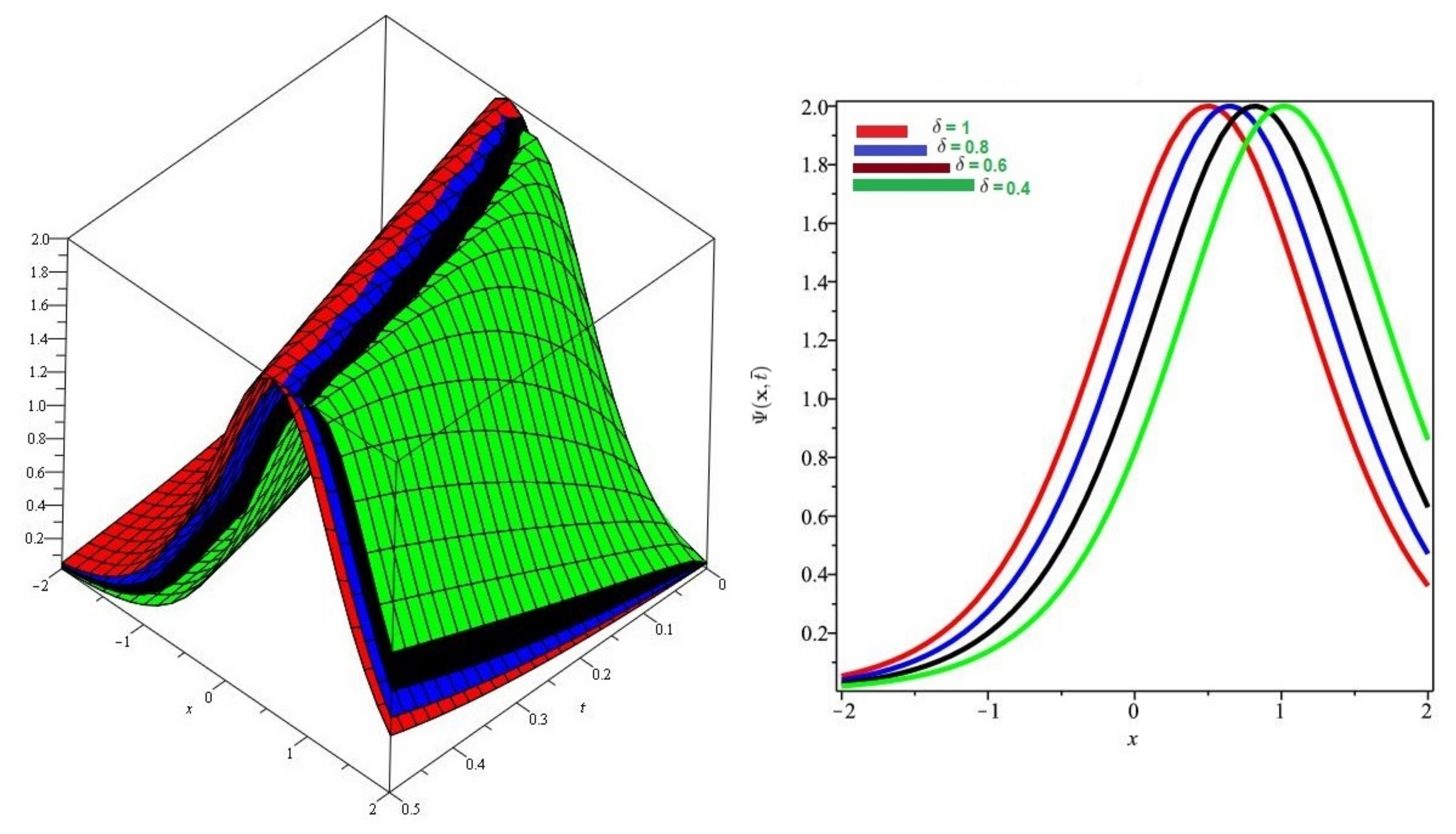
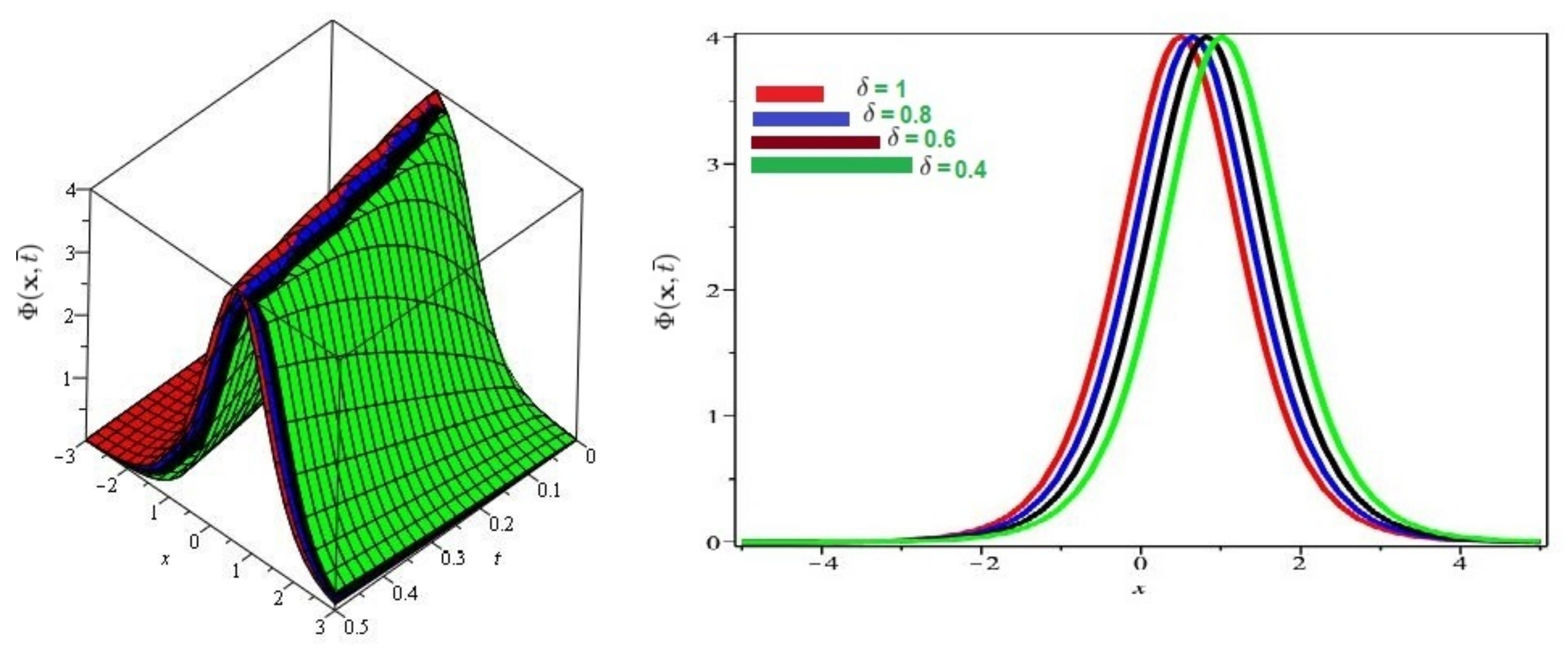
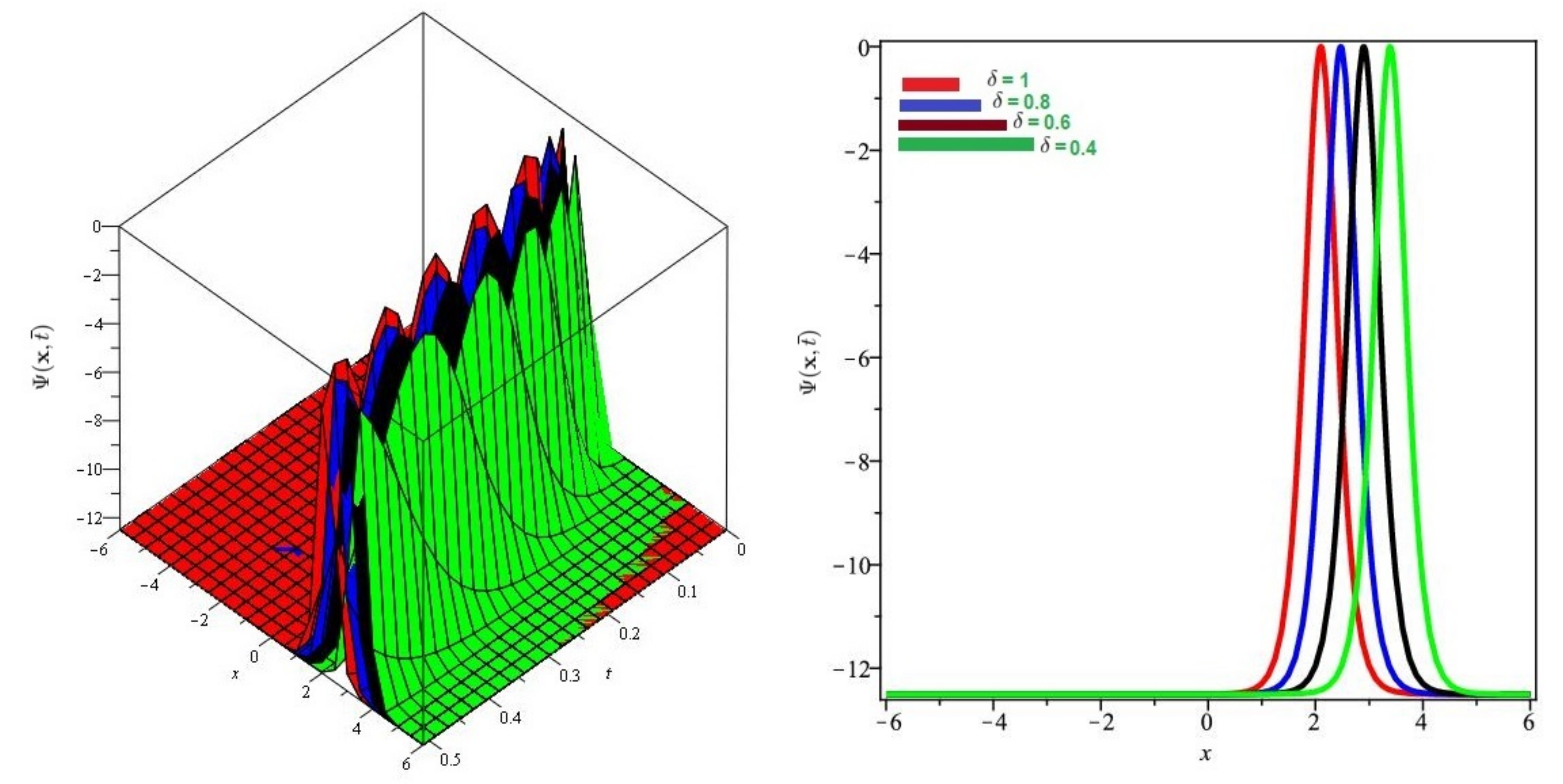
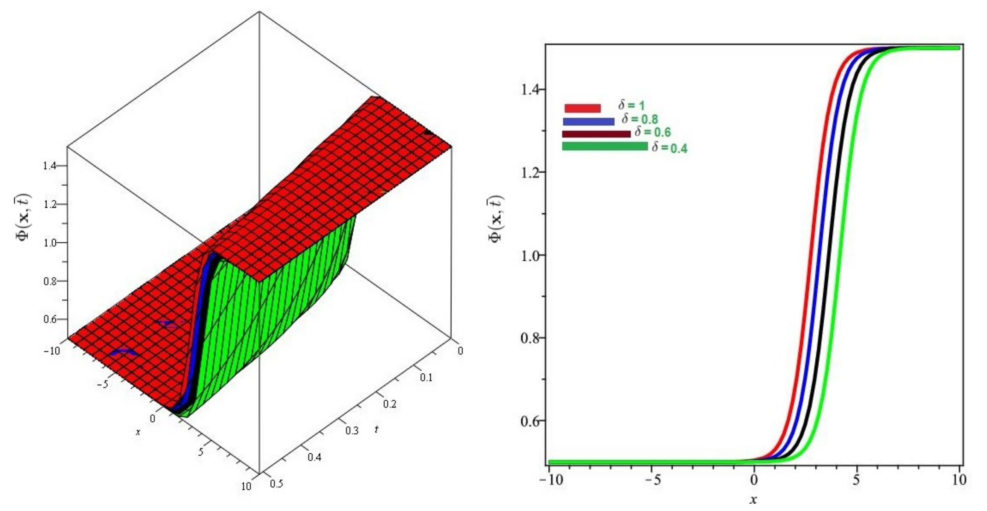
6. Evaluation of the Fractional KdV Model

This section represents some test examples by employing two novel methods, SDM and SITM via the Caputo derivative operator. Furthermore, the convergence and stability of the method are elaborated on.

Problem 1

([16]). Assume the time-fractional coupled nonlinear KdV Equation (1) with $\sigma =\zeta =1,$ subject to the condition

$$\begin{array}{c}\hfill \Phi (\mathbf{x},0)={\ell }^{2}sec{h}^2\left(\frac{\beta }{2}+\frac{\ell \mathbf{x}}{2}\right),\Psi (\mathbf{x},0)=\sqrt{\frac{\sigma }{2}}{\ell }^{2}sec{h}^2\left(\frac{\beta }{2}+\frac{\ell \mathbf{x}}{2}\right).\end{array}$$

(31)

Case I. First, we surmise the Shehu decomposition method for Problem 1.

Employing the Shehu transformation to (1), we find

$$\begin{array}{ccc}& & \frac{{\xi }^{\delta }}{{\omega }^{\delta }}\mathcal{U}(\xi ,\omega )-\sum _{\kappa =0}^{m-1}{\left(\frac{\xi }{\omega }\right)}^{\delta -\kappa -1}{\Phi }^{\left(\kappa \right)}\left(0\right)=\mathbb{S}\left[-\sigma \frac{{\partial }^3\Phi }{\partial {\mathbf{x}}^3}-6\sigma \Phi \frac{\partial \Phi }{\partial \mathbf{x}}+6\Psi \frac{\partial \Psi }{\partial \mathbf{x}}\right],\hfill \\ & & \frac{{\xi }^{\delta }}{{\omega }^{\delta }}\mathcal{V}(\xi ,\omega )-\sum _{\kappa =0}^{m-1}{\left(\frac{\xi }{\omega }\right)}^{\delta -\kappa -1}{\Psi }^{\left(\kappa \right)}\left(0\right)=\mathbb{S}\left[-\sigma \frac{{\partial }^3\Psi }{\partial {\mathbf{x}}^3}-3\sigma \Phi \frac{\partial \Psi }{\partial \mathbf{x}}\right].\hfill \end{array}$$

(32)

In view of (31) and simple computations yield

$$\begin{array}{ccc}& & \mathcal{U}(\xi ,\omega )=\frac{\omega }{\xi }{\Phi }^{\left(0\right)}(\mathbf{x},0)+\frac{{\omega }^{\delta }}{{\xi }^{\delta }}\mathbb{S}\left[-\sigma \frac{{\partial }^3\Phi }{\partial {\mathbf{x}}^3}-6\sigma \Phi \frac{\partial \Phi }{\partial \mathbf{x}}+6\Psi \frac{\partial \Psi }{\partial \mathbf{x}}\right],\hfill \\ & & \mathcal{V}(\xi ,\omega )=\frac{\omega }{\xi }{\Psi }^{\left(0\right)}(\mathbf{x},0)+\frac{{\omega }^{\delta }}{{\xi }^{\delta }}\mathbb{S}\left[-\sigma \frac{{\partial }^3\Psi }{\partial {\mathbf{x}}^3}-3\sigma \Phi \frac{\partial \Psi }{\partial \mathbf{x}}\right].\hfill \end{array}$$

Applying the inverse Shehu transform, we have

$$\begin{array}{ccc}\hfill & & \Phi (\mathbf{x},\overline{t})={\mathbb{S}}^{-1}\left[\frac{\omega }{\xi }\Phi (\mathbf{x},0)\right]+{\mathbb{S}}^{-1}\left[\frac{{\omega }^{\delta }}{{\xi }^{\delta }}\mathbb{S}\left[-\sigma \frac{{\partial }^3\Phi }{\partial {\mathbf{x}}^3}-6\sigma \Phi \frac{\partial \Phi }{\partial \mathbf{x}}+6\Psi \frac{\partial \Psi }{\partial \mathbf{x}}\right]\right],\hfill \\ & & \Psi (\mathbf{x},\overline{t})={\mathbb{S}}^{-1}\left[\frac{\omega }{\xi }\Psi (\mathbf{x},0)\right]+{\mathbb{S}}^{-1}\left[\frac{{\omega }^{\delta }}{{\xi }^{\delta }}\mathbb{S}\left[-\sigma \frac{{\partial }^3\Psi }{\partial {\mathbf{x}}^3}-3\sigma \Phi \frac{\partial \Psi }{\partial \mathbf{x}}\right]\right].\hfill \end{array}$$

(33)

By virtue of the Shehu decomposition method, we have

$$\begin{array}{ccc}\hfill {\Phi }_0(\mathbf{x},\overline{t})& & ={\mathbb{S}}^{-1}\left[\frac{\omega }{\xi }\Phi (\mathbf{x},0)\right]={\mathbb{S}}^{-1}\left[\frac{\xi }{\omega }{\ell }^{2}sec{h}^2\left(\frac{\beta }{2}+\frac{\ell \mathbf{x}}{2}\right)\right]\hfill \\ & & ={\ell }^{2}sec{h}^2\left(\frac{\beta }{2}+\frac{\ell \mathbf{x}}{2}\right),\hfill \\ \hfill {\Psi }_0(\mathbf{x},\overline{t})& & ={\mathbb{S}}^{-1}\left[\frac{\omega }{\xi }\Psi (\mathbf{x},0)\right]\hfill \\ & & =\sqrt{\frac{\sigma }{2}}{\ell }^{2}sec{h}^2\left(\frac{\beta }{2}+\frac{\ell \mathbf{x}}{2}\right).\hfill \end{array}$$

$$\begin{array}{ccc}\hfill \sum _{m=0}^{\infty }{\Phi }_{m+1}(\mathbf{x},\overline{t})& & ={\mathbb{S}}^{-1}\left[\frac{{\omega }^{\delta }}{{\xi }^{\delta }}\mathbb{S}\left[-\sigma \sum _{m=0}^{\infty }{\left({\Phi }_{\mathbf{x}\mathbf{x}\mathbf{x}}\right)}_m-6\sigma \sum _{m=0}^{\infty }{\mathcal{A}}_m+6\sum _{m=0}^{\infty }{\mathcal{B}}_m\right]\right],\hfill \\ \hfill \sum _{m=0}^{\infty }{\Psi }_{m+1}(\mathbf{x},\overline{t})& & ={\mathbb{S}}^{-1}\left[\frac{{\omega }^{\delta }}{{\xi }^{\delta }}\mathbb{S}\left[-\sigma \sum _{m=0}^{\infty }{\left({\Psi }_{\mathbf{x}\mathbf{x}\mathbf{x}}\right)}_m-3\sigma \sum _{m=0}^{\infty }{\mathcal{C}}_m\right]\right],m=0,1,2,....\hfill \end{array}$$

The first few Adomian polynomials are presented as follows:

$$\begin{array}{ccc}\hfill {\mathcal{A}}_0(\Phi {\Phi }_{\mathbf{x}})& & ={\Phi }_0{\Phi }_{0\mathbf{x}},\hfill \\ \hfill {\mathcal{A}}_1(\Phi {\Phi }_{\mathbf{x}})& & ={\Phi }_0{\Phi }_{1\mathbf{x}}+{\Phi }_1{\Phi }_{0\mathbf{x}},\hfill \\ \hfill {\mathcal{A}}_2(\Phi {\Phi }_{\mathbf{x}})& & ={\Phi }_1{\Phi }_{2\mathbf{x}}+{\Phi }_1{\Phi }_{1\mathbf{x}}+{\Phi }_2{\Phi }_{0\mathbf{x}},\hfill \\ \hfill {\mathcal{B}}_0(\Psi {\Psi }_{\mathbf{x}})& & ={\Psi }_0{\Psi }_{0\mathbf{x}},\hfill \\ \hfill {\mathcal{B}}_1(\Psi {\Psi }_{\mathbf{x}})& & ={\Psi }_0{\Psi }_{1\mathbf{x}}+{\Psi }_1{\Psi }_{0\mathbf{x}},\hfill \\ \hfill {\mathcal{B}}_2(\Psi {\Psi }_{\mathbf{x}})& & ={\Psi }_1{\Psi }_{2\mathbf{x}}+{\Psi }_1{\Psi }_{1\mathbf{x}}+{\Psi }_2{\Psi }_{0\mathbf{x}},\hfill \\ \hfill {\mathcal{C}}_0(\Phi {\Psi }_{\mathbf{x}})& & ={\Phi }_0{\Psi }_{0\mathbf{x}},\hfill \\ \hfill {\mathcal{C}}_1(\Phi {\Psi }_{\mathbf{x}})& & ={\Phi }_0{\Psi }_{1\mathbf{x}}+{\Phi }_1{\Psi }_{0\mathbf{x}},\hfill \\ \hfill {\mathcal{C}}_2(\Phi {\Psi }_{\mathbf{x}})& & ={\Phi }_1{\Psi }_{2\mathbf{x}}+{\Phi }_1{\Psi }_{1\mathbf{x}}+{\Phi }_2{\Psi }_{0\mathbf{x}}.\hfill \end{array}$$

For $m=0,1,2,3,...$

$$\begin{array}{ccc}\hfill {\Phi }_1(\mathbf{x},\overline{t})& & ={\mathbb{S}}^{-1}\left[\frac{{\omega }^{\delta }}{{\xi }^{\delta }}\mathbb{S}\left[-\sigma {\left({\Phi }_{\mathbf{x}\mathbf{x}\mathbf{x}}\right)}_0-6\sigma {\mathcal{A}}_0+6{\mathcal{B}}_0\right]\right]\hfill \\ & & ={\mathbb{S}}^{-1}\left[\frac{{\omega }^{\delta +2}}{{\xi }^{\delta +2}}{\ell }^5\sigma tanh\left(\frac{\beta }{2}+\frac{\ell \mathbf{x}}{2}\right)sec{h}^2\left(\frac{\beta }{2}+\frac{\ell \mathbf{x}}{2}\right)\right]\hfill \\ & & ={\ell }^5\sigma tanh\left(\frac{\beta }{2}+\frac{\ell \mathbf{x}}{2}\right)sec{h}^2\left(\frac{\beta }{2}+\frac{\ell \mathbf{x}}{2}\right)\frac{{\overline{t}}^{\delta }}{\Gamma (\delta +1)},\hfill \\ \hfill {\Psi }_1(\mathbf{x},\overline{t})& & ={\mathbb{S}}^{-1}\left[\frac{{\omega }^{\delta }}{{\xi }^{\delta }}\mathbb{S}\left[-\sigma {\left({\Psi }_{\mathbf{x}\mathbf{x}\mathbf{x}}\right)}_0-3\sigma {\mathcal{C}}_0\right]\right]\hfill \\ & & =\frac{{\ell }^5{\sigma }^{3/2}}{\sqrt{2}}tanh\left(\frac{\beta }{2}+\frac{\ell \mathbf{x}}{2}\right)sec{h}^2\left(\frac{\beta }{2}+\frac{\ell \mathbf{x}}{2}\right)\frac{{\overline{t}}^{\delta }}{\Gamma (\delta +1)}.\hfill \\ \hfill {\Phi }_2(\mathbf{x},\overline{t})& & ={\mathbb{S}}^{-1}\left[\frac{{\omega }^{\delta }}{{\xi }^{\delta }}\mathbb{S}\left[-\sigma {\left({\Phi }_{\mathbf{x}\mathbf{x}\mathbf{x}}\right)}_1-6\sigma {\mathcal{A}}_1+6{\mathcal{B}}_1\right]\right]\hfill \\ & & ={\mathbb{S}}^{-1}\left[\frac{{\omega }^{2\delta +2}}{{\xi }^{2\delta +2}}\frac{{\ell }^8{\sigma }^2}{2}\left[2{cosh}^2\left(\frac{\sigma }{2}+\frac{\ell \mathbf{x}}{2}\right)-3\right]sec{h}^4\left(\frac{\sigma }{2}+\frac{\ell \mathbf{x}}{2}\right)\right]\hfill \\ & & =\frac{{\ell }^8{\sigma }^2}{2}\left[2{cosh}^2\left(\frac{\sigma }{2}+\frac{\ell \mathbf{x}}{2}\right)-3\right]sec{h}^4\left(\frac{\sigma }{2}+\frac{\ell \mathbf{x}}{2}\right)\frac{{\overline{t}}^{2\delta }}{\Gamma (2\delta +1)},\hfill \\ \hfill {\Psi }_2(\mathbf{x},\overline{t})& & ={\mathbb{S}}^{-1}\left[\frac{{\omega }^{\delta }}{{\xi }^{\delta }}\mathbb{S}\left[-\sigma {\left({\Psi }_{\mathbf{x}\mathbf{x}\mathbf{x}}\right)}_1-3\sigma {\mathcal{C}}_1\right]\right]\hfill \\ & & =\frac{{\ell }^5{\sigma }^{5/2}}{2\sqrt{2}}\left[2{cosh}^2\left(\frac{\sigma }{2}+\frac{\ell \mathbf{x}}{2}\right)-3\right]sec{h}^4\left(\frac{\sigma }{2}+\frac{\ell \mathbf{x}}{2}\right)\frac{{\overline{t}}^{2\delta }}{\Gamma (2\delta +1)},\hfill \end{array}$$

$$\begin{array}{ccc}\hfill {\Phi }_3(\mathbf{x},\overline{t})& & ={\mathbb{S}}^{-1}\left[\frac{{\omega }^{\delta }}{{\xi }^{\delta }}\mathbb{S}\left[-\sigma {\left({\Phi }_{\mathbf{x}\mathbf{x}\mathbf{x}}\right)}_2-6\sigma {\mathcal{A}}_2+6{\mathcal{B}}_2\right]\right]\hfill \\ & & =\frac{{\sigma }^3{\ell }^{4}sinh\left(\frac{\sigma }{2}+\frac{\ell \mathbf{x}}{2}\right)}{2{\Gamma }^2(\delta +1)\Gamma (3\delta +1){cosh}^7\left(\frac{\beta }{2}+\frac{\ell \mathbf{x}}{2}\right)}[2{\Gamma }^2(\delta +1)cos{h}^4\left(\frac{\sigma }{2}+\frac{\ell \mathbf{x}}{2}\right)-18{\Gamma }^2(\delta +1)cos{h}^2\left(\frac{\sigma }{2}+\frac{\ell \mathbf{x}}{2}\right)\hfill \\ & & +6\Gamma (2\delta +1)cos{h}^2\left(\frac{\sigma }{2}+\frac{\ell \mathbf{x}}{2}\right)+18{\Gamma }^2(\delta +1)-9\Gamma (2\delta +1)],\hfill \\ \hfill {\Psi }_3(\mathbf{x},\overline{t})& & ={\mathbb{S}}^{-1}\left[\frac{{\omega }^{\delta }}{{\xi }^{\delta }}\mathbb{S}\left[-\sigma {\left({\Psi }_{\mathbf{x}\mathbf{x}\mathbf{x}}\right)}_2-3\sigma {\mathcal{C}}_2\right]\right]\hfill \\ & & =\frac{{\sigma }^{7/2}{\ell }^{11}sinh\left(\frac{\sigma }{2}+\frac{\ell \mathbf{x}}{2}\right)}{2\sqrt{2}{\Gamma }^2(\delta +1)\Gamma (3\delta +1){cosh}^7\left(\frac{\beta }{2}+\frac{\ell \mathbf{x}}{2}\right)}[2{\Gamma }^2(\delta +1)cos{h}^4\left(\frac{\sigma }{2}+\frac{\ell \mathbf{x}}{2}\right)-18{\Gamma }^2(\delta +1)cos{h}^2\left(\frac{\sigma }{2}+\frac{\ell \mathbf{x}}{2}\right)\hfill \\ & & +6\Gamma (2\delta +1)cos{h}^2\left(\frac{\sigma }{2}+\frac{\ell \mathbf{x}}{2}\right)+18{\Gamma }^2(\delta +1)-9\Gamma (2\delta +1)],\hfill \\ \hfill ⋮.\end{array}$$

The Shehu decomposition method solution for Problem 1 is presented as:

$$\begin{array}{ccc}\hfill \Phi (\mathbf{x},\overline{t})& & ={\Phi }_0(\mathbf{x},\overline{t})+{\Phi }_1(\mathbf{x},\overline{t})+{\Phi }_2(\mathbf{x},\overline{t})+{\Phi }_3(\mathbf{x},\overline{t})+...,\hfill \\ & & ={\ell }^{2}sec{h}^2\left(\frac{\beta }{2}+\frac{\ell \mathbf{x}}{2}\right)+{\ell }^5\sigma tanh\left(\frac{\beta }{2}+\frac{\ell \mathbf{x}}{2}\right)sec{h}^2\left(\frac{\beta }{2}+\frac{\ell \mathbf{x}}{2}\right)\frac{{\overline{t}}^{\delta }}{\Gamma (\delta +1)}\hfill \\ & & +\frac{{\ell }^8{\sigma }^2}{2}\left[2{cosh}^2\left(\frac{\sigma }{2}+\frac{\ell \mathbf{x}}{2}\right)-3\right]sec{h}^4\left(\frac{\sigma }{2}+\frac{\ell \mathbf{x}}{2}\right)\frac{{\overline{t}}^{2\delta }}{\Gamma (2\delta +1)}\hfill \\ & & +\frac{{\sigma }^3{\ell }^{4}sinh\left(\frac{\sigma }{2}+\frac{\ell \mathbf{x}}{2}\right)}{2{\Gamma }^2(\delta +1)\Gamma (3\delta +1){cosh}^7\left(\frac{\beta }{2}+\frac{\ell \mathbf{x}}{2}\right)}[2{\Gamma }^2(\delta +1)cos{h}^4\left(\frac{\sigma }{2}+\frac{\ell \mathbf{x}}{2}\right)-18{\Gamma }^2(\delta +1)cos{h}^2\left(\frac{\sigma }{2}+\frac{\ell \mathbf{x}}{2}\right)\hfill \\ & & +6\Gamma (2\delta +1)cos{h}^2\left(\frac{\sigma }{2}+\frac{\ell \mathbf{x}}{2}\right)+18{\Gamma }^2(\delta +1)-9\Gamma (2\delta +1)]+....\hfill \end{array}$$

Analogously, we have

$$\begin{array}{ccc}\hfill \Psi (\mathbf{x},\overline{t})& & =\sqrt{\frac{\sigma }{2}}{\ell }^{2}sec{h}^2\left(\frac{\beta }{2}+\frac{\ell \mathbf{x}}{2}\right)+\frac{{\ell }^5{\sigma }^{3/2}}{\sqrt{2}}tanh\left(\frac{\beta }{2}+\frac{\ell \mathbf{x}}{2}\right)sec{h}^2\left(\frac{\beta }{2}+\frac{\ell \mathbf{x}}{2}\right)\frac{{\overline{t}}^{\delta }}{\Gamma (\delta +1)}\hfill \\ & & +\frac{{\ell }^5{\sigma }^{5/2}}{2\sqrt{2}}\left[2{cosh}^2\left(\frac{\sigma }{2}+\frac{\ell \mathbf{x}}{2}\right)-3\right]sec{h}^4\left(\frac{\sigma }{2}+\frac{\ell \mathbf{x}}{2}\right)\frac{{\overline{t}}^{2\delta }}{\Gamma (2\delta +1)}\hfill \\ & & +\frac{{\sigma }^{7/2}{\ell }^{11}sinh\left(\frac{\sigma }{2}+\frac{\ell \mathbf{x}}{2}\right)}{2\sqrt{2}{\Gamma }^2(\delta +1)\Gamma (3\delta +1){cosh}^7\left(\frac{\beta }{2}+\frac{\ell \mathbf{x}}{2}\right)}[2{\Gamma }^2(\delta +1)cos{h}^4\left(\frac{\sigma }{2}+\frac{\ell \mathbf{x}}{2}\right)-18{\Gamma }^2(\delta +1)cos{h}^2\left(\frac{\sigma }{2}+\frac{\ell \mathbf{x}}{2}\right)\hfill \\ & & +6\Gamma (2\delta +1)cos{h}^2\left(\frac{\sigma }{2}+\frac{\ell \mathbf{x}}{2}\right)+18{\Gamma }^2(\delta +1)-9\Gamma (2\delta +1)]+....\hfill \end{array}$$

By setting $\delta =1,$ we then obtain the exact solution of coupled KdV Equation (1)

$$\begin{array}{ccc}\hfill \Phi (\mathbf{x},\overline{t})& & ={\ell }^{2}sec{h}^2\left(\frac{\beta }{2}+\frac{\ell \mathbf{x}}{2}-\frac{\sigma {\ell }^3\overline{t}}{2}\right),\hfill \\ \hfill \Psi (\mathbf{x},\overline{t})& & =\sqrt{\frac{\sigma }{2}}{\ell }^{2}sec{h}^2\left(\frac{\beta }{2}+\frac{\ell \mathbf{x}}{2}-\frac{\sigma {\ell }^3\overline{t}}{2}\right).\hfill \end{array}$$

Case II. Now, we surmise the Shehu iterative transform method on Problem 1.

Applying the proposed analytical approach to (33), yields

$$\begin{array}{ccc}\hfill {\Phi }_0(\mathbf{x},\overline{t})& & ={\mathbb{S}}^{-1}\left[\frac{\omega }{\xi }\Phi (\mathbf{x},0)\right]={\mathbb{S}}^{-1}\left[\frac{\xi }{\omega }{\ell }^{2}sec{h}^2\left(\frac{\beta }{2}+\frac{\ell \mathbf{x}}{2}\right)\right]\hfill \\ & & ={\ell }^{2}sec{h}^2\left(\frac{\beta }{2}+\frac{\ell \mathbf{x}}{2}\right),\hfill \\ \hfill {\Psi }_0(\mathbf{x},\overline{t})& & ={\mathbb{S}}^{-1}\left[\frac{\omega }{\xi }\Psi (\mathbf{x},0)\right]\hfill \\ & & =\sqrt{\frac{\sigma }{2}}{\ell }^{2}sec{h}^2\left(\frac{\beta }{2}+\frac{\ell \mathbf{x}}{2}\right).\hfill \\ \hfill {\Phi }_1(\mathbf{x},\overline{t})& & ={\mathbb{S}}^{-1}\left[\frac{{\omega }^{\delta }}{{\xi }^{\delta }}\mathbb{S}\left[-\sigma \frac{{\partial }^3{\Phi }_0}{\partial {\mathbf{x}}^3}-6\sigma {\Phi }_0\frac{\partial {\Phi }_0}{\partial \mathbf{x}}+6{\Psi }_0\frac{\partial {\Psi }_0}{\partial \mathbf{x}}\right]\right]\hfill \\ & & ={\mathbb{S}}^{-1}\left[\frac{{\omega }^{\delta +2}}{{\xi }^{\delta +2}}{\ell }^5\sigma tanh\left(\frac{\beta }{2}+\frac{\ell \mathbf{x}}{2}\right)sec{h}^2\left(\frac{\beta }{2}+\frac{\ell \mathbf{x}}{2}\right)\right]\hfill \\ & & ={\ell }^5\sigma tanh\left(\frac{\beta }{2}+\frac{\ell \mathbf{x}}{2}\right)sec{h}^2\left(\frac{\beta }{2}+\frac{\ell \mathbf{x}}{2}\right)\frac{{\overline{t}}^{\delta }}{\Gamma (\delta +1)},\hfill \\ \hfill {\Psi }_1(\mathbf{x},\overline{t})& & ={\mathbb{S}}^{-1}\left[\frac{{\omega }^{\delta }}{{\xi }^{\delta }}\mathbb{S}\left[-\sigma \frac{{\partial }^3{\Psi }_0}{\partial {\mathbf{x}}^3}-3\sigma {\Phi }_0\frac{\partial {\Psi }_0}{\partial \mathbf{x}}\right]\right]\hfill \\ & & =\frac{{\ell }^5{\sigma }^{3/2}}{\sqrt{2}}tanh\left(\frac{\beta }{2}+\frac{\ell \mathbf{x}}{2}\right)sec{h}^2\left(\frac{\beta }{2}+\frac{\ell \mathbf{x}}{2}\right)\frac{{\overline{t}}^{\delta }}{\Gamma (\delta +1)}.\hfill \\ \hfill {\Phi }_2(\mathbf{x},\overline{t})& & ={\mathbb{S}}^{-1}\left[\frac{{\omega }^{\delta }}{{\xi }^{\delta }}\mathbb{S}\left[-\sigma \frac{{\partial }^3{\Phi }_1}{\partial {\mathbf{x}}^3}-6\sigma {\Phi }_1\frac{\partial {\Phi }_1}{\partial \mathbf{x}}+6{\Psi }_1\frac{\partial {\Psi }_1}{\partial \mathbf{x}}\right]\right]\hfill \\ & & ={\mathbb{S}}^{-1}\left[\frac{{\omega }^{2\delta +2}}{{\xi }^{2\delta +2}}\frac{{\ell }^8{\sigma }^2}{2}\left[2{cosh}^2\left(\frac{\sigma }{2}+\frac{\ell \mathbf{x}}{2}\right)-3\right]sec{h}^4\left(\frac{\sigma }{2}+\frac{\ell \mathbf{x}}{2}\right)\right]\hfill \\ & & =\frac{{\ell }^8{\sigma }^2}{2}\left[2{cosh}^2\left(\frac{\sigma }{2}+\frac{\ell \mathbf{x}}{2}\right)-3\right]sec{h}^4\left(\frac{\sigma }{2}+\frac{\ell \mathbf{x}}{2}\right)\frac{{\overline{t}}^{2\delta }}{\Gamma (2\delta +1)},\hfill \\ \hfill {\Psi }_2(\mathbf{x},\overline{t})& & ={\mathbb{S}}^{-1}\left[\frac{{\omega }^{\delta }}{{\xi }^{\delta }}\mathbb{S}\left[-\sigma \frac{{\partial }^3{\Psi }_1}{\partial {\mathbf{x}}^3}-3\sigma {\Phi }_1\frac{\partial {\Psi }_1}{\partial \mathbf{x}}\right]\right]\hfill \\ & & =\frac{{\ell }^5{\sigma }^{5/2}}{2\sqrt{2}}\left[2{cosh}^2\left(\frac{\sigma }{2}+\frac{\ell \mathbf{x}}{2}\right)-3\right]sec{h}^4\left(\frac{\sigma }{2}+\frac{\ell \mathbf{x}}{2}\right)\frac{{\overline{t}}^{2\delta }}{\Gamma (2\delta +1)},\hfill \end{array}$$

$$\begin{array}{ccc}\hfill {\Phi }_3(\mathbf{x},\overline{t})& & ={\mathbb{S}}^{-1}\left[\frac{{\omega }^{\delta }}{{\xi }^{\delta }}\mathbb{S}\left[-\sigma \frac{{\partial }^3{\Phi }_2}{\partial {\mathbf{x}}^3}-6\sigma {\Phi }_2\frac{\partial {\Phi }_2}{\partial \mathbf{x}}+6{\Psi }_2\frac{\partial {\Psi }_2}{\partial \mathbf{x}}\right]\right]\hfill \\ & & =\frac{{\sigma }^3{\ell }^{4}sinh\left(\frac{\sigma }{2}+\frac{\ell \mathbf{x}}{2}\right)}{2{\Gamma }^2(\delta +1)\Gamma (3\delta +1){cosh}^7\left(\frac{\beta }{2}+\frac{\ell \mathbf{x}}{2}\right)}[2{\Gamma }^2(\delta +1)cos{h}^4\left(\frac{\sigma }{2}+\frac{\ell \mathbf{x}}{2}\right)-18{\Gamma }^2(\delta +1)cos{h}^2\left(\frac{\sigma }{2}+\frac{\ell \mathbf{x}}{2}\right)\hfill \\ & & +6\Gamma (2\delta +1)cos{h}^2\left(\frac{\sigma }{2}+\frac{\ell \mathbf{x}}{2}\right)+18{\Gamma }^2(\delta +1)-9\Gamma (2\delta +1)],\hfill \\ \hfill {\Psi }_3(\mathbf{x},\overline{t})& & ={\mathbb{S}}^{-1}\left[\frac{{\omega }^{\delta }}{{\xi }^{\delta }}\mathbb{S}\left[-\sigma \frac{{\partial }^3{\Psi }_2}{\partial {\mathbf{x}}^3}-3\sigma {\Phi }_2\frac{\partial {\Psi }_2}{\partial \mathbf{x}}\right]\right]\hfill \\ & & =\frac{{\sigma }^{7/2}{\ell }^{11}sinh\left(\frac{\sigma }{2}+\frac{\ell \mathbf{x}}{2}\right)}{2\sqrt{2}{\Gamma }^2(\delta +1)\Gamma (3\delta +1){cosh}^7\left(\frac{\beta }{2}+\frac{\ell \mathbf{x}}{2}\right)}[2{\Gamma }^2(\delta +1)cos{h}^4\left(\frac{\sigma }{2}+\frac{\ell \mathbf{x}}{2}\right)-18{\Gamma }^2(\delta +1)cos{h}^2\left(\frac{\sigma }{2}+\frac{\ell \mathbf{x}}{2}\right)\hfill \\ & & +6\Gamma (2\delta +1)cos{h}^2\left(\frac{\sigma }{2}+\frac{\ell \mathbf{x}}{2}\right)+18{\Gamma }^2(\delta +1)-9\Gamma (2\delta +1)],\hfill \\ & & ⋮\hfill \end{array}$$

$$\begin{array}{ccc}\hfill {\Phi }_n(\mathbf{x},\overline{t})& & ={\mathbb{S}}^{-1}\left[\frac{{\omega }^{\delta }}{{\xi }^{\delta }}\mathbb{S}\left[-\sigma \frac{{\partial }^3{\Phi }_{m-1}}{\partial {\mathbf{x}}^3}-6\sigma {\Phi }_{m-1}\frac{\partial {\Phi }_{m-1}}{\partial \mathbf{x}}+6{\Psi }_{m-1}\frac{\partial {\Psi }_{m-1}}{\partial \mathbf{x}}\right]\right],\hfill \\ \hfill {\Psi }_m(\mathbf{x},\overline{t})& & ={\mathbb{S}}^{-1}\left[\frac{{\omega }^{\delta }}{{\xi }^{\delta }}\mathbb{S}\left[-\sigma \frac{{\partial }^3{\Psi }_{m-1}}{\partial {\mathbf{x}}^3}-3\sigma {\Phi }_{m-1}\frac{\partial {\Psi }_{m-1}}{\partial \mathbf{x}}\right]\right].\hfill \end{array}$$

The series of solutions for Problem 1 is presented as:

$$\begin{array}{ccc}\hfill \Phi (\mathbf{x},\overline{t})& & ={\Phi }_0(\mathbf{x},\overline{t})+{\Phi }_1(\mathbf{x},\overline{t})+{\Phi }_2(\mathbf{x},\overline{t})+{\Phi }_3(\mathbf{x},\overline{t})+...{\Phi }_m(\mathbf{x},\overline{t}),\hfill \\ \hfill \Psi (\mathbf{x},\overline{t})& & ={\Psi }_0(\mathbf{x},\overline{t})+{\Psi }_1(\mathbf{x},\overline{t})+{\Psi }_2(\mathbf{x},\overline{t})+{\Psi }_3(\mathbf{x},\overline{t})+...{\Psi }_m(\mathbf{x},\overline{t}).\hfill \end{array}$$

Consequently, we have

$$\begin{array}{ccc}\hfill \Phi (\mathbf{x},\overline{t})& & ={\ell }^{2}sec{h}^2\left(\frac{\beta }{2}+\frac{\ell \mathbf{x}}{2}\right)+{\ell }^5\sigma tanh\left(\frac{\beta }{2}+\frac{\ell \mathbf{x}}{2}\right)sec{h}^2\left(\frac{\beta }{2}+\frac{\ell \mathbf{x}}{2}\right)\frac{{\overline{t}}^{\delta }}{\Gamma (\delta +1)}\hfill \\ & & +\frac{{\ell }^8{\sigma }^2}{2}\left[2{cosh}^2\left(\frac{\sigma }{2}+\frac{\ell \mathbf{x}}{2}\right)-3\right]sec{h}^4\left(\frac{\sigma }{2}+\frac{\ell \mathbf{x}}{2}\right)\frac{{\overline{t}}^{2\delta }}{\Gamma (2\delta +1)}\hfill \\ & & +\frac{{\sigma }^3{\ell }^{4}sinh\left(\frac{\sigma }{2}+\frac{\ell \mathbf{x}}{2}\right)}{2{\Gamma }^2(\delta +1)\Gamma (3\delta +1){cosh}^7\left(\frac{\beta }{2}+\frac{\ell \mathbf{x}}{2}\right)}[2{\Gamma }^2(\delta +1)cos{h}^4\left(\frac{\sigma }{2}+\frac{\ell \mathbf{x}}{2}\right)-18{\Gamma }^2(\delta +1)cos{h}^2\left(\frac{\sigma }{2}+\frac{\ell \mathbf{x}}{2}\right)\hfill \\ & & +6\Gamma (2\delta +1)cos{h}^2\left(\frac{\sigma }{2}+\frac{\ell \mathbf{x}}{2}\right)+18{\Gamma }^2(\delta +1)-9\Gamma (2\delta +1)]+...,\hfill \\ \hfill \Psi (\mathbf{x},\overline{t})& & =\sqrt{\frac{\sigma }{2}}{\ell }^{2}sec{h}^2\left(\frac{\beta }{2}+\frac{\ell \mathbf{x}}{2}\right)+\frac{{\ell }^5{\sigma }^{3/2}}{\sqrt{2}}tanh\left(\frac{\beta }{2}+\frac{\ell \mathbf{x}}{2}\right)sec{h}^2\left(\frac{\beta }{2}+\frac{\ell \mathbf{x}}{2}\right)\frac{{\overline{t}}^{\delta }}{\Gamma (\delta +1)}\hfill \\ & & +\frac{{\ell }^5{\sigma }^{5/2}}{2\sqrt{2}}\left[2{cosh}^2\left(\frac{\sigma }{2}+\frac{\ell \mathbf{x}}{2}\right)-3\right]sec{h}^4\left(\frac{\sigma }{2}+\frac{\ell \mathbf{x}}{2}\right)\frac{{\overline{t}}^{2\delta }}{\Gamma (2\delta +1)}\hfill \\ & & +\frac{{\sigma }^{7/2}{\ell }^{11}sinh\left(\frac{\sigma }{2}+\frac{\ell \mathbf{x}}{2}\right)}{2\sqrt{2}{\Gamma }^2(\delta +1)\Gamma (3\delta +1){cosh}^7\left(\frac{\beta }{2}+\frac{\ell \mathbf{x}}{2}\right)}[2{\Gamma }^2(\delta +1)cos{h}^4\left(\frac{\sigma }{2}+\frac{\ell \mathbf{x}}{2}\right)-18{\Gamma }^2(\delta +1)cos{h}^2\left(\frac{\sigma }{2}+\frac{\ell \mathbf{x}}{2}\right)\hfill \\ & & +6\Gamma (2\delta +1)cos{h}^2\left(\frac{\sigma }{2}+\frac{\ell \mathbf{x}}{2}\right)+18{\Gamma }^2(\delta +1)-9\Gamma (2\delta +1)]+....\hfill \end{array}$$

By setting $\delta =1,$ we then obtain the exact solution of coupled KdV Equation (1)

$$\begin{array}{ccc}\hfill \Phi (\mathbf{x},\overline{t})& & ={\ell }^{2}sec{h}^2\left(\frac{\beta }{2}+\frac{\ell \mathbf{x}}{2}-\frac{\sigma {\ell }^3\overline{t}}{2}\right),\hfill \\ \hfill \Psi (\mathbf{x},\overline{t})& & =\sqrt{\frac{\sigma }{2}}{\ell }^{2}sec{h}^2\left(\frac{\beta }{2}+\frac{\ell \mathbf{x}}{2}-\frac{\sigma {\ell }^3\overline{t}}{2}\right).\hfill \end{array}$$

In Figure 1 and Figure 2, the exact and approximate results of $\Phi (\mathbf{x},\overline{t})$ and $\Psi (\mathbf{x},\overline{t})$ are demonstrated at $\ell =1,\sigma =0.5$ and $\beta =2.$ In Figure 3 and Figure 4, the surface and 2D graph for $\Phi (\mathbf{x},\overline{t})$ and $\Psi (\mathbf{x},\overline{t})$ for various fractional order are presented which shows that the SDM/SITM approximated results derived are in a strong agreement with the exact and the numerical ones. This comparison represents a strong correlation between the SDM and exact findings. Therefore, the SDM/SITM are reliable novel approaches which require less computation time and is quite straightforward and more flexible than the homotopy perturbation method and homotopy analysis method.

Problem 2

([16]). Assume the time-fractional coupled nonlinear KdV equation is presented as:

$$\begin{array}{ccc}\hfill \frac{{\partial }^{\delta }\Phi }{\partial {\overline{t}}^{\delta }}& & =-\frac{\partial \Psi }{\partial \mathbf{x}}-\frac{1}{2}\frac{\partial {\Phi }^2}{\partial \mathbf{x}}\hfill \\ \hfill \frac{{\partial }^{\delta }\Psi }{\partial {\overline{t}}^{\delta }}& & =-\frac{\partial \Phi }{\partial \mathbf{x}}-\frac{{\partial }^3\Phi }{\partial {\mathbf{x}}^3}-\frac{\partial \Phi \Psi }{\partial \mathbf{x}},\overline{t}>0,0<\delta \le 1\hfill \end{array}$$

(34)

subject to the condition

$$\begin{array}{c}\hfill \Phi (\mathbf{x},0)=\sigma \left[tanh\left(\frac{\ell }{2}+\frac{\sigma \mathbf{x}}{2}\right)+1\right],\Psi (\mathbf{x},0)=\frac{{\sigma }^2}{2}sec{h}^2\left(\frac{\ell }{2}+\frac{\sigma \mathbf{x}}{2}\right)-1.\end{array}$$

(35)

Case I. First, we surmise the Shehu decomposition method for Problem 2.

Employing the Shehu transformation to (34), we find

$$\begin{array}{ccc}& & \frac{{\xi }^{\delta }}{{\omega }^{\delta }}\mathcal{U}(\xi ,\omega )-\sum _{\kappa =0}^{m-1}{\left(\frac{\xi }{\omega }\right)}^{\delta -\kappa -1}{\Phi }^{\left(\kappa \right)}\left(0\right)=\mathbb{S}\left[-\frac{\partial \Psi }{\partial \mathbf{x}}-\frac{1}{2}\frac{\partial {\Phi }^2}{\partial \mathbf{x}}\right],\hfill \\ & & \frac{{\xi }^{\delta }}{{\omega }^{\delta }}\mathcal{V}(\xi ,\omega )-\sum _{\kappa =0}^{m-1}{\left(\frac{\xi }{\omega }\right)}^{\delta -\kappa -1}{\Psi }^{\left(\kappa \right)}\left(0\right)=\mathbb{S}\left[-\frac{\partial \Phi }{\partial \mathbf{x}}-\frac{{\partial }^3\Phi }{\partial {\mathbf{x}}^3}-\frac{\partial \Phi \Psi }{\partial \mathbf{x}}\right].\hfill \end{array}$$

(36)

In view of (35) and simple computations yield

$$\begin{array}{ccc}& & \mathcal{U}(\xi ,\omega )=\frac{\omega }{\xi }{\Phi }^{\left(0\right)}(\mathbf{x},0)+\frac{{\omega }^{\delta }}{{\xi }^{\delta }}\mathbb{S}\left[-\frac{\partial \Psi }{\partial \mathbf{x}}-\frac{1}{2}\frac{\partial {\Phi }^2}{\partial \mathbf{x}}\right],\hfill \\ & & \mathcal{V}(\xi ,\omega )=\frac{\omega }{\xi }{\Psi }^{\left(0\right)}(\mathbf{x},0)+\frac{{\omega }^{\delta }}{{\xi }^{\delta }}\mathbb{S}\left[-\frac{\partial \Phi }{\partial \mathbf{x}}-\frac{{\partial }^3\Phi }{\partial {\mathbf{x}}^3}-\frac{\partial \Phi \Psi }{\partial \mathbf{x}}\right].\hfill \end{array}$$

(37)

Applying the inverse Shehu transform, we have

$$\begin{array}{ccc}\hfill & & \Phi (\mathbf{x},\overline{t})={\mathbb{S}}^{-1}\left[\frac{\omega }{\xi }\Phi (\mathbf{x},0)\right]+{\mathbb{S}}^{-1}\left[\frac{{\omega }^{\delta }}{{\xi }^{\delta }}\mathbb{S}\left[-\frac{\partial \Psi }{\partial \mathbf{x}}-\frac{1}{2}\frac{\partial {\Phi }^2}{\partial \mathbf{x}}\right]\right],\hfill \\ & & \Psi (\mathbf{x},\overline{t})={\mathbb{S}}^{-1}\left[\frac{\omega }{\xi }\Psi (\mathbf{x},0)\right]+{\mathbb{S}}^{-1}\left[\frac{{\omega }^{\delta }}{{\xi }^{\delta }}\mathbb{S}\left[-\frac{\partial \Phi }{\partial \mathbf{x}}-\frac{{\partial }^3\Phi }{\partial {\mathbf{x}}^3}-\frac{\partial \Phi \Psi }{\partial \mathbf{x}}\right]\right].\hfill \end{array}$$

(38)

By virtue of the Shehu decomposition method, we have

$$\begin{array}{ccc}\hfill {\Phi }_0(\mathbf{x},\overline{t})& & ={\mathbb{S}}^{-1}\left[\frac{\omega }{\xi }\Phi (\mathbf{x},0)\right]={\mathbb{S}}^{-1}\left[\frac{\omega }{\xi }\sigma \left(tanh\left(\frac{\ell }{2}+\frac{\sigma \mathbf{x}}{2}\right)+1\right)\right]\hfill \\ & & =\sigma \left(tanh\left(\frac{\ell }{2}+\frac{\sigma \mathbf{x}}{2}\right)+1\right),\hfill \\ \hfill {\Psi }_0(\mathbf{x},\overline{t})& & ={\mathbb{S}}^{-1}\left[\frac{\omega }{\xi }\Psi (\mathbf{x},0)\right]\hfill \\ & & =\frac{{\sigma }^2}{2}sec{h}^2\left(\frac{\ell }{2}+\frac{\sigma \mathbf{x}}{2}\right)-1.\hfill \end{array}$$

It follows that

$$\begin{array}{ccc}\hfill \sum _{m=0}^{\infty }{\Phi }_{m+1}(\mathbf{x},\overline{t})& & ={\mathbb{S}}^{-1}\left[\frac{{\omega }^{\delta }}{{\xi }^{\delta }}\mathbb{S}\left[-\sigma \sum _{m=0}^{\infty }{\left({\Psi }_{\mathbf{x}}\right)}_m-\frac{1}{2}\sum _{m=0}^{\infty }{\mathcal{D}}_m\right]\right],\hfill \\ \hfill \sum _{m=0}^{\infty }{\Psi }_{m+1}(\mathbf{x},\overline{t})& & ={\mathbb{S}}^{-1}\left[\frac{{\omega }^{\delta }}{{\xi }^{\delta }}\mathbb{S}\left[-\sum _{m=0}^{\infty }{\left({\Phi }_{\mathbf{x}}\right)}_m-\sum _{m=0}^{\infty }{\left({\Psi }_{\mathbf{x}\mathbf{x}\mathbf{x}}\right)}_m-\sum _{m=0}^{\infty }{\left({(\Phi \Psi )}_{\mathbf{x}}\right)}_m\right]\right],m=0,1,2,....\hfill \end{array}$$

The first few Adomian polynomials are presented as follows:

$$\begin{array}{ccc}\hfill {\mathcal{D}}_0\left({\Phi }^2\right)& & ={\Phi }_0^2,\hfill \\ \hfill {\mathcal{D}}_1\left({\Phi }^2\right)& & =2{\Phi }_0{\Phi }_1,\hfill \\ \hfill {\mathcal{D}}_2\left({\Phi }^2\right)& & =2{\Phi }_0{\Phi }_2+{\Phi }_1^2.\hfill \end{array}$$

For $m=0,1,2,...$

$$\begin{array}{ccc}\hfill {\Phi }_1(\mathbf{x},\overline{t})& & ={\mathbb{S}}^{-1}\left[\frac{{\omega }^{\delta }}{{\xi }^{\delta }}\mathbb{S}\left[-\sigma {\left({\Psi }_{\mathbf{x}}\right)}_0-\frac{1}{2}{\mathcal{D}}_0\right]\right]\hfill \\ & & =-\frac{{\sigma }^2}{2}{\mathbb{S}}^{-1}\left[\frac{{\omega }^{\delta +2}}{{\xi }^{\delta +2}}sec{h}^2\left(\frac{\ell }{2}+\frac{\sigma \mathbf{x}}{2}\right)\right]\hfill \\ & & =-\frac{{\sigma }^2}{2}sec{h}^2\left(\frac{\ell }{2}+\frac{\sigma \mathbf{x}}{2}\right)\frac{{\overline{t}}^{\delta }}{\Gamma (\delta +1)},\hfill \\ \hfill {\Psi }_1(\mathbf{x},\overline{t})& & ={\mathbb{S}}^{-1}\left[\frac{{\omega }^{\delta }}{{\xi }^{\delta }}\mathbb{S}\left[-{\left({\Phi }_{\mathbf{x}}\right)}_0-{\left({\Psi }_{\mathbf{x}\mathbf{x}\mathbf{x}}\right)}_0-{\left({(\Phi \Psi )}_{\mathbf{x}}\right)}_0\right]\right]\hfill \\ & & =\frac{{\sigma }^3}{2}sinh\left(\frac{\ell }{2}+\frac{\sigma \mathbf{x}}{2}\right)sec{h}^3\left(\frac{\ell }{2}+\frac{\sigma \mathbf{x}}{2}\right)\frac{{\overline{t}}^{\delta }}{\Gamma (\delta +1)}.\hfill \end{array}$$

$$\begin{array}{ccc}\hfill {\Phi }_2(\mathbf{x},\overline{t})& & ={\mathbb{S}}^{-1}\left[\frac{{\omega }^{\delta }}{{\xi }^{\delta }}\mathbb{S}\left[-\sigma {\left({\Psi }_{\mathbf{x}}\right)}_1-\frac{1}{2}{\mathcal{D}}_1\right]\right]\hfill \\ & & ={\mathbb{S}}^{-1}\left[-\frac{{\sigma }^5}{4}\frac{{\omega }^{2\delta +2}}{{\xi }^{2\delta +2}}sec{h}^2\left(\frac{\ell }{2}+\frac{\sigma \mathbf{x}}{2}\right)+\frac{3{\sigma }^5}{4}\frac{{\omega }^{2\delta +2}}{{\xi }^{2\delta +2}}sin{h}^2\left(\frac{\ell }{2}+\frac{\sigma \mathbf{x}}{2}\right)sec{h}^4\left(\frac{\ell }{2}+\frac{\sigma \mathbf{x}}{2}\right)\right]\hfill \\ & & +\frac{{\sigma }^7}{4}{\mathbb{S}}^{-1}\left[\frac{\Gamma (2\delta +1)}{{\Gamma }^2(\delta +1)}\frac{{\omega }^{3\delta +2}}{{\xi }^{3\delta +2}}sinh\left(\frac{\ell }{2}+\frac{\sigma \mathbf{x}}{2}\right)sec{h}^5\left(\frac{\ell }{2}+\frac{\sigma \mathbf{x}}{2}\right)\right]\hfill \\ & & =\left[-\frac{{\sigma }^5}{4}sec{h}^2\left(\frac{\ell }{2}+\frac{\sigma \mathbf{x}}{2}\right)+\frac{3{\sigma }^5}{4}sin{h}^2\left(\frac{\ell }{2}+\frac{\sigma \mathbf{x}}{2}\right)sec{h}^4\left(\frac{\ell }{2}+\frac{\sigma \mathbf{x}}{2}\right)\right]\frac{{\overline{t}}^{2\delta }}{\Gamma (2\delta +1)}\hfill \\ & & +\frac{{\sigma }^7}{4}sinh\left(\frac{\ell }{2}+\frac{\sigma \mathbf{x}}{2}\right)sec{h}^5\left(\frac{\ell }{2}+\frac{\sigma \mathbf{x}}{2}\right)\frac{\Gamma (2\delta +1){\overline{t}}^{3\delta }}{{\Gamma }^2(\delta +1)\Gamma (3\delta +1)},\hfill \end{array}$$

$$\begin{array}{ccc}\hfill {\Psi }_2(\mathbf{x},\overline{t})& & ={\mathbb{S}}^{-1}\left[\frac{{\omega }^{\delta }}{{\xi }^{\delta }}\left[-{\left({\Phi }_{\mathbf{x}}\right)}_1-{\left({\Psi }_{\mathbf{x}\mathbf{x}\mathbf{x}}\right)}_1-{\left({(\Phi \Psi )}_{\mathbf{x}}\right)}_1\right]\right]\hfill \\ & & =\frac{{\sigma }^6}{4}\left[2{cosh}^2\left(\frac{\ell }{2}+\frac{\sigma \mathbf{x}}{2}\right)-3\right]sec{h}^4\left(\frac{\ell }{2}+\frac{\sigma \mathbf{x}}{2}\right)\frac{{\overline{t}}^{2\delta }}{\Gamma (2\delta +1)},\hfill \\ \hfill ⋮.\end{array}$$

The Shehu decomposition method solution for Problem 2 is presented as:

$$\begin{array}{ccc}\hfill \Phi (\mathbf{x},\overline{t})& & ={\Phi }_0(\mathbf{x},\overline{t})+{\Phi }_1(\mathbf{x},\overline{t})+{\Phi }_2(\mathbf{x},\overline{t})+...,\hfill \\ & & =\sigma \left(tanh\left(\frac{\ell }{2}+\frac{\sigma \mathbf{x}}{2}\right)+1\right)-\frac{{\sigma }^2}{2}sec{h}^2\left(\frac{\ell }{2}+\frac{\sigma \mathbf{x}}{2}\right)\frac{{\overline{t}}^{\delta }}{\Gamma (\delta +1)}\hfill \\ & & +\left[-\frac{{\sigma }^5}{4}sec{h}^2\left(\frac{\ell }{2}+\frac{\sigma \mathbf{x}}{2}\right)+\frac{3{\sigma }^5}{4}sin{h}^2\left(\frac{\ell }{2}+\frac{\sigma \mathbf{x}}{2}\right)sec{h}^4\left(\frac{\ell }{2}+\frac{\sigma \mathbf{x}}{2}\right)\right]\frac{{\overline{t}}^{2\delta }}{\Gamma (2\delta +1)}\hfill \\ & & +\frac{{\sigma }^7}{4}sinh\left(\frac{\ell }{2}+\frac{\sigma \mathbf{x}}{2}\right)sec{h}^5\left(\frac{\ell }{2}+\frac{\sigma \mathbf{x}}{2}\right)\frac{\Gamma (2\delta +1){\overline{t}}^{3\delta }}{{\Gamma }^2(\delta +1)\Gamma (3\delta +1)}+....\hfill \end{array}$$

Analogously, we have

$$\begin{array}{ccc}\hfill \Psi (\mathbf{x},\overline{t})& & =-1+\frac{{\sigma }^2}{2}sec{h}^2\left(\frac{\ell }{2}+\frac{\sigma \mathbf{x}}{2}\right)+\frac{{\sigma }^3}{2}sinh\left(\frac{\ell }{2}+\frac{\sigma \mathbf{x}}{2}\right)sec{h}^3\left(\frac{\ell }{2}+\frac{\sigma \mathbf{x}}{2}\right)\frac{{\overline{t}}^{\delta }}{\Gamma (\delta +1)}\hfill \\ & & +\frac{{\sigma }^6}{4}\left[2{cosh}^2\left(\frac{\ell }{2}+\frac{\sigma \mathbf{x}}{2}\right)-3\right]sec{h}^4\left(\frac{\ell }{2}+\frac{\sigma \mathbf{x}}{2}\right)\frac{{\overline{t}}^{2\delta }}{\Gamma (2\delta +1)}+....\hfill \end{array}$$

By setting $\delta =1,$ we obtain the exact solution of the coupled KdV Equation (34)

$$\begin{array}{ccc}\hfill \Phi (\mathbf{x},\overline{t})& & =\sigma \left(tanh\left(\frac{\ell }{2}+\frac{\sigma \mathbf{x}}{2}-\frac{{\sigma }^2\overline{t}}{2}\right)+1\right),\hfill \\ \hfill \Psi (\mathbf{x},\overline{t})& & =\frac{{\sigma }^2}{2}sec{h}^2\left(\frac{\ell }{2}+\frac{\sigma \mathbf{x}}{2}-\frac{{\sigma }^2\overline{t}}{2}\right)-1.\hfill \end{array}$$

Case II. Now, we surmise the Shehu iterative transform method on Problem 2.

Applying the proposed analytical approach to (38) yields

$$\begin{array}{ccc}\hfill {\Phi }_0(\mathbf{x},\overline{t})& & ={\mathbb{S}}^{-1}\left[\frac{\omega }{\xi }\Phi (\mathbf{x},0)\right]={\mathbb{S}}^{-1}\left[\frac{\omega }{\xi }\sigma \left(tanh\left(\frac{\ell }{2}+\frac{\sigma \mathbf{x}}{2}\right)+1\right)\right]\hfill \\ & & =\sigma \left(tanh\left(\frac{\ell }{2}+\frac{\sigma \mathbf{x}}{2}\right)+1\right),\hfill \\ \hfill {\Psi }_0(\mathbf{x},\overline{t})& & ={\mathbb{S}}^{-1}\left[\frac{\omega }{\xi }\Psi (\mathbf{x},0)\right]\hfill \\ & & =\frac{{\sigma }^2}{2}sec{h}^2\left(\frac{\ell }{2}+\frac{\sigma \mathbf{x}}{2}\right)-1\hfill \\ \hfill {\Phi }_1(\mathbf{x},\overline{t})& & ={\mathbb{S}}^{-1}\left[\frac{{\omega }^{\delta }}{{\xi }^{\delta }}\mathbb{S}\left[-\frac{\partial {\Psi }_0}{\partial \mathbf{x}}-\frac{1}{2}\frac{\partial {\Phi }_0^2}{\partial \mathbf{x}}\right]\right]\hfill \\ & & =-\frac{{\sigma }^2}{2}{\mathbb{S}}^{-1}\left[\frac{{\omega }^{\delta +2}}{{\xi }^{\delta +2}}sec{h}^2\left(\frac{\ell }{2}+\frac{\sigma \mathbf{x}}{2}\right)\right]\hfill \\ & & =-\frac{{\sigma }^2}{2}sec{h}^2\left(\frac{\ell }{2}+\frac{\sigma \mathbf{x}}{2}\right)\frac{{\overline{t}}^{\delta }}{\Gamma (\delta +1)},\hfill \end{array}$$

$$\begin{array}{ccc}\hfill {\Psi }_1(\mathbf{x},\overline{t})& & ={\mathbb{S}}^{-1}\left[\frac{{\omega }^{\delta }}{{\xi }^{\delta }}\mathbb{S}\left[-\frac{\partial {\Phi }_0}{\partial \mathbf{x}}-\frac{{\partial }^3{\Phi }_0}{\partial {\mathbf{x}}^3}-\frac{\partial {\Phi }_0{\Psi }_0}{\partial \mathbf{x}}\right]\right]\hfill \\ & & =\frac{{\sigma }^3}{2}sinh\left(\frac{\ell }{2}+\frac{\sigma \mathbf{x}}{2}\right)sec{h}^3\left(\frac{\ell }{2}+\frac{\sigma \mathbf{x}}{2}\right)\frac{{\overline{t}}^{\delta }}{\Gamma (\delta +1)},\hfill \end{array}$$

$$\begin{array}{ccc}\hfill {\Phi }_2(\mathbf{x},\overline{t})& & ={\mathbb{S}}^{-1}\left[\frac{{\omega }^{\delta }}{{\xi }^{\delta }}\mathbb{S}\left[-\frac{\partial {\Psi }_1}{\partial \mathbf{x}}-\frac{1}{2}\frac{\partial {\Phi }_1^2}{\partial \mathbf{x}}\right]\right]\hfill \\ & & ={\mathbb{S}}^{-1}\left[-\frac{{\sigma }^5}{4}\frac{{\omega }^{2\delta +2}}{{\xi }^{2\delta +2}}sec{h}^2\left(\frac{\ell }{2}+\frac{\sigma \mathbf{x}}{2}\right)+\frac{3{\sigma }^5}{4}\frac{{\omega }^{2\delta +2}}{{\xi }^{2\delta +2}}sin{h}^2\left(\frac{\ell }{2}+\frac{\sigma \mathbf{x}}{2}\right)sec{h}^4\left(\frac{\ell }{2}+\frac{\sigma \mathbf{x}}{2}\right)\right]\hfill \\ & & +\frac{{\sigma }^7}{4}{\mathbb{S}}^{-1}\left[\frac{\Gamma (2\delta +1)}{{\Gamma }^2(\delta +1)}\frac{{\omega }^{3\delta +2}}{{\xi }^{3\delta +2}}sinh\left(\frac{\ell }{2}+\frac{\sigma \mathbf{x}}{2}\right)sec{h}^5\left(\frac{\ell }{2}+\frac{\sigma \mathbf{x}}{2}\right)\right]\hfill \\ & & =\left[-\frac{{\sigma }^5}{4}sec{h}^2\left(\frac{\ell }{2}+\frac{\sigma \mathbf{x}}{2}\right)+\frac{3{\sigma }^5}{4}sin{h}^2\left(\frac{\ell }{2}+\frac{\sigma \mathbf{x}}{2}\right)sec{h}^4\left(\frac{\ell }{2}+\frac{\sigma \mathbf{x}}{2}\right)\right]\frac{{\overline{t}}^{2\delta }}{\Gamma (2\delta +1)}\hfill \\ & & +\frac{{\sigma }^7}{4}sinh\left(\frac{\ell }{2}+\frac{\sigma \mathbf{x}}{2}\right)sec{h}^5\left(\frac{\ell }{2}+\frac{\sigma \mathbf{x}}{2}\right)\frac{\Gamma (2\delta +1){\overline{t}}^{3\delta }}{{\Gamma }^2(\delta +1)\Gamma (3\delta +1)},\hfill \end{array}$$

$$\begin{array}{ccc}\hfill {\Psi }_2(\mathbf{x},\overline{t})& & ={\mathbb{S}}^{-1}\left[\frac{{\omega }^{\delta }}{{\xi }^{\delta }}\left[-\frac{\partial {\Phi }_1}{\partial \mathbf{x}}-\frac{{\partial }^3{\Phi }_1}{\partial {\mathbf{x}}^3}-\frac{\partial {\Phi }_1{\Psi }_1}{\partial \mathbf{x}}\right]\right]\hfill \\ & & =\frac{{\sigma }^6}{4}\left[2{cosh}^2\left(\frac{\ell }{2}+\frac{\sigma \mathbf{x}}{2}\right)-3\right]sec{h}^4\left(\frac{\ell }{2}+\frac{\sigma \mathbf{x}}{2}\right)\frac{{\overline{t}}^{2\delta }}{\Gamma (2\delta +1)},\hfill \\ & & ⋮\hfill \\ \hfill {\Phi }_m(\mathbf{x},\overline{t})& & ={\mathbb{S}}^{-1}\left[\frac{{\omega }^{\delta }}{{\xi }^{\delta }}\mathbb{S}\left[-\frac{\partial {\Psi }_{m-1}}{\partial \mathbf{x}}-\frac{1}{2}\frac{\partial {\Phi }_{m-1}^2}{\partial \mathbf{x}}\right]\right],\hfill \\ \hfill {\Psi }_m(\mathbf{x},\overline{t})& & ={\mathbb{S}}^{-1}\left[\frac{{\omega }^{\delta }}{{\xi }^{\delta }}\left[-\frac{\partial {\Phi }_{m-1}}{\partial \mathbf{x}}-\frac{{\partial }^3{\Phi }_{m-1}}{\partial {\mathbf{x}}^3}-\frac{\partial {\Phi }_{m-1}{\Psi }_{m-1}}{\partial \mathbf{x}}\right]\right].\hfill \end{array}$$

The series of solution for Problem 2 is presented as:

$$\begin{array}{ccc}\hfill \Phi (\mathbf{x},\overline{t})& & ={\Phi }_0(\mathbf{x},\overline{t})+{\Phi }_1(\mathbf{x},\overline{t})+{\Phi }_2(\mathbf{x},\overline{t})+...{\Phi }_m(\mathbf{x},\overline{t}),\hfill \\ \hfill \Psi (\mathbf{x},\overline{t})& & ={\Psi }_0(\mathbf{x},\overline{t})+{\Psi }_1(\mathbf{x},\overline{t})+{\Psi }_2(\mathbf{x},\overline{t})+...{\Psi }_m(\mathbf{x},\overline{t}).\hfill \end{array}$$

Consequently, we have

$$\begin{array}{ccc}\hfill \Phi (\mathbf{x},\overline{t})& & =\sigma \left(tanh\left(\frac{\ell }{2}+\frac{\sigma \mathbf{x}}{2}\right)+1\right)-\frac{{\sigma }^2}{2}sec{h}^2\left(\frac{\ell }{2}+\frac{\sigma \mathbf{x}}{2}\right)\frac{{\overline{t}}^{\delta }}{\Gamma (\delta +1)}\hfill \\ & & +\left[-\frac{{\sigma }^5}{4}sec{h}^2\left(\frac{\ell }{2}+\frac{\sigma \mathbf{x}}{2}\right)+\frac{3{\sigma }^5}{4}sin{h}^2\left(\frac{\ell }{2}+\frac{\sigma \mathbf{x}}{2}\right)sec{h}^4\left(\frac{\ell }{2}+\frac{\sigma \mathbf{x}}{2}\right)\right]\frac{{\overline{t}}^{2\delta }}{\Gamma (2\delta +1)}\hfill \\ & & +\frac{{\sigma }^7}{4}sinh\left(\frac{\ell }{2}+\frac{\sigma \mathbf{x}}{2}\right)sec{h}^5\left(\frac{\ell }{2}+\frac{\sigma \mathbf{x}}{2}\right)\frac{\Gamma (2\delta +1){\overline{t}}^{3\delta }}{{\Gamma }^2(\delta +1)\Gamma (3\delta +1)}+...,\hfill \\ \hfill \Psi (\mathbf{x},\overline{t})& & =-1+\frac{{\sigma }^2}{2}sec{h}^2\left(\frac{\ell }{2}+\frac{\sigma \mathbf{x}}{2}\right)+\frac{{\sigma }^3}{2}sinh\left(\frac{\ell }{2}+\frac{\sigma \mathbf{x}}{2}\right)sec{h}^3\left(\frac{\ell }{2}+\frac{\sigma \mathbf{x}}{2}\right)\frac{{\overline{t}}^{\delta }}{\Gamma (\delta +1)}\hfill \\ & & +\frac{{\sigma }^6}{4}\left[2{cosh}^2\left(\frac{\ell }{2}+\frac{\sigma \mathbf{x}}{2}\right)-3\right]sec{h}^4\left(\frac{\ell }{2}+\frac{\sigma \mathbf{x}}{2}\right)\frac{{\overline{t}}^{2\delta }}{\Gamma (2\delta +1)}+....\hfill \end{array}$$

By setting $\delta =1,$ we then obtain the exact solution of coupled KdV Equation (34)

$$\begin{array}{ccc}\hfill \Phi (\mathbf{x},\overline{t})& & =\sigma \left(tanh\left(\frac{\ell }{2}+\frac{\sigma \mathbf{x}}{2}-\frac{{\sigma }^2\overline{t}}{2}\right)+1\right),\hfill \\ \hfill \Psi (\mathbf{x},\overline{t})& & =\frac{{\sigma }^2}{2}sec{h}^2\left(\frac{\ell }{2}+\frac{\sigma \mathbf{x}}{2}-\frac{{\sigma }^2\overline{t}}{2}\right)-1.\hfill \end{array}$$

In Figure 5 and Figure 6, the exact and approximate results of $\Phi (\mathbf{x},\overline{t})$ and $\Psi (\mathbf{x},\overline{t})$ are demonstrated at $\ell =1,\sigma =0.5$ and $\beta =2.$ In Figure 7 and Figure 8, the surface and 2D graph for $\Phi (\mathbf{x},\overline{t})$ and $\Psi (\mathbf{x},\overline{t})$ for various fractional order are presented which shows that the SDM/SITM approximated results derived are in a strong agreement with the exact and the numerical ones. This comparison represents a strong correlation between the SDM and exact findings. Therefore, the SDM/SITM are reliable novel approaches which require less computation time and are quite straightforward and more flexible than the homotopy perturbation method and the homotopy analysis method.

Problem 3

([16]). Assume the time-fractional coupled nonlinear MCKdV equations is presented as (2) subject to the condition

$$\begin{array}{c}\hfill \Phi (\mathbf{x},0)=\frac{2+tanh\mathbf{x}}{2},\Psi (\mathbf{x},0)=\frac{2-tanh\mathbf{x}}{4},\mathsf{{\rm Y}}(\mathbf{x},0)=2-tanh\mathbf{x}.\end{array}$$

(39)

Case I. First, we surmise the Shehu decomposition method for Problem 3.

Employing the Shehu transformation to (2), we find

$$\begin{array}{ccc}\hfill \frac{{\xi }^{\delta }}{{\omega }^{\delta }}\mathcal{U}(\xi ,\omega )-\sum _{\kappa =0}^{m-1}{\left(\frac{\xi }{\omega }\right)}^{\delta -\kappa -1}{\Phi }^{\left(\kappa \right)}\left(0\right)& & =\mathbb{S}[\frac{1}{2}\frac{{\partial }^3\Phi }{\partial {\overline{t}}^3}-3{\Phi }^2\frac{\partial \Phi }{\partial \mathbf{x}}+\frac{3}{2}\mathsf{{\rm Y}}\frac{{\partial }^2\Psi }{\partial {\mathbf{x}}^2}+3\frac{\partial \Psi }{\partial \mathbf{x}}\frac{\partial \mathsf{{\rm Y}}}{\partial \mathbf{x}}+\frac{3}{2}\Psi \frac{{\partial }^2\mathsf{{\rm Y}}}{\partial {\mathbf{x}}^2}\hfill \\ & & +3\Psi \mathsf{{\rm Y}}\frac{\partial \Phi }{\partial \mathbf{x}}+3\Phi \mathsf{{\rm Y}}\frac{\partial \Psi }{\partial \mathbf{x}}+3\Phi \Psi \frac{\partial \mathsf{{\rm Y}}}{\partial \mathbf{x}}],\hfill \\ \hfill \frac{{\xi }^{\delta }}{{\omega }^{\delta }}\mathcal{V}(\xi ,\omega )-\sum _{\kappa =0}^{m-1}{\left(\frac{\xi }{\omega }\right)}^{\delta -\kappa -1}{\Psi }^{\left(\kappa \right)}\left(0\right)& & =\mathbb{S}\left[-\frac{{\partial }^3\Psi }{\partial {\mathbf{x}}^3}-3\frac{\partial \Phi }{\partial \mathbf{x}}\frac{\partial \Psi }{\partial \mathbf{x}}-3\Psi \frac{{\partial }^2\Phi }{\partial {\mathbf{x}}^2}-3{\Psi }^2\frac{\partial \mathsf{{\rm Y}}}{\partial \mathbf{x}}+6\Phi \Psi \frac{\partial \Phi }{\partial \mathbf{x}}+3{\Phi }^2\frac{\partial \Psi }{\partial \mathbf{x}}\right],\hfill \\ \hfill \frac{{\xi }^{\delta }}{{\omega }^{\delta }}\mathcal{W}(\xi ,\omega )-\sum _{\kappa =0}^{m-1}{\left(\frac{\xi }{\omega }\right)}^{\delta -\kappa -1}{\mathsf{{\rm Y}}}^{\left(\kappa \right)}\left(0\right)& & =\mathbb{S}\left[-\frac{{\partial }^3\mathsf{{\rm Y}}}{\partial {\mathbf{x}}^3}-3\frac{\partial \Phi }{\partial \mathbf{x}}\frac{\partial \mathsf{{\rm Y}}}{\partial \mathbf{x}}-3\mathsf{{\rm Y}}\frac{{\partial }^2\Phi }{\partial {\mathbf{x}}^2}-3{\mathsf{{\rm Y}}}^2\frac{\partial \Psi }{\partial \mathbf{x}}+6\Phi \mathsf{{\rm Y}}\frac{\partial \Phi }{\partial \mathbf{x}}+3{\Phi }^2\frac{\partial \mathsf{{\rm Y}}}{\partial \mathbf{x}}\right].\hfill \end{array}$$

(40)

In view of (39) and simple computations yield

$$\begin{array}{ccc}\hfill \mathcal{U}(\xi ,\omega )& & =\frac{\omega }{\xi }{\Phi }^{\left(0\right)}(\mathbf{x},0)+\frac{{\omega }^{\delta }}{{\xi }^{\delta }}\mathbb{S}[\frac{1}{2}\frac{{\partial }^3\Phi }{\partial {\overline{t}}^3}-3{\Phi }^2\frac{\partial \Phi }{\partial \mathbf{x}}+\frac{3}{2}\mathsf{{\rm Y}}\frac{{\partial }^2\Psi }{\partial {\mathbf{x}}^2}+3\frac{\partial \Psi }{\partial \mathbf{x}}\frac{\partial \mathsf{{\rm Y}}}{\partial \mathbf{x}}+\frac{3}{2}\Psi \frac{{\partial }^2\mathsf{{\rm Y}}}{\partial {\mathbf{x}}^2}\hfill \\ & & +3\Psi \mathsf{{\rm Y}}\frac{\partial \Phi }{\partial \mathbf{x}}+3\Phi \mathsf{{\rm Y}}\frac{\partial \Psi }{\partial \mathbf{x}}+3\Phi \Psi \frac{\partial \mathsf{{\rm Y}}}{\partial \mathbf{x}}],\hfill \\ \hfill \mathcal{V}(\xi ,\omega )& & =\frac{\omega }{\xi }{\Psi }^{\left(0\right)}(\mathbf{x},0)+\frac{{\omega }^{\delta }}{{\xi }^{\delta }}\mathbb{S}\left[-\frac{{\partial }^3\Psi }{\partial {\mathbf{x}}^3}-3\frac{\partial \Phi }{\partial \mathbf{x}}\frac{\partial \Psi }{\partial \mathbf{x}}-3\Psi \frac{{\partial }^2\Phi }{\partial {\mathbf{x}}^2}-3{\Psi }^2\frac{\partial \mathsf{{\rm Y}}}{\partial \mathbf{x}}+6\Phi \Psi \frac{\partial \Phi }{\partial \mathbf{x}}+3{\Phi }^2\frac{\partial \Psi }{\partial \mathbf{x}}\right],\hfill \\ \hfill \mathcal{W}(\xi ,\omega )& & =\frac{\omega }{\xi }{\mathsf{{\rm Y}}}^{\left(0\right)}(\mathbf{x},0)+\frac{{\omega }^{\delta }}{{\xi }^{\delta }}\mathbb{S}\left[-\frac{{\partial }^3\mathsf{{\rm Y}}}{\partial {\mathbf{x}}^3}-3\frac{\partial \Phi }{\partial \mathbf{x}}\frac{\partial \mathsf{{\rm Y}}}{\partial \mathbf{x}}-3\mathsf{{\rm Y}}\frac{{\partial }^2\Phi }{\partial {\mathbf{x}}^2}-3{\mathsf{{\rm Y}}}^2\frac{\partial \Psi }{\partial \mathbf{x}}+6\Phi \mathsf{{\rm Y}}\frac{\partial \Phi }{\partial \mathbf{x}}+3{\Phi }^2\frac{\partial \mathsf{{\rm Y}}}{\partial \mathbf{x}}\right].\hfill \end{array}$$

(41)

Applying the inverse Shehu transform, we have

$$\begin{array}{ccc}\hfill \Phi (\mathbf{x},\overline{t})& & ={\mathbb{S}}^{-1}\left[\frac{\omega }{\xi }\Phi (\mathbf{x},0)\right]+{\mathbb{S}}^{-1}\left[\frac{{\omega }^{\delta }}{{\xi }^{\delta }}\mathbb{S}\right[\frac{1}{2}\frac{{\partial }^3\Phi }{\partial {\overline{t}}^3}-3{\Phi }^2\frac{\partial \Phi }{\partial \mathbf{x}}+\frac{3}{2}\mathsf{{\rm Y}}\frac{{\partial }^2\Psi }{\partial {\mathbf{x}}^2}+3\frac{\partial \Psi }{\partial \mathbf{x}}\frac{\partial \mathsf{{\rm Y}}}{\partial \mathbf{x}}+\frac{3}{2}\Psi \frac{{\partial }^2\mathsf{{\rm Y}}}{\partial {\mathbf{x}}^2}\hfill \\ & & +3\Psi \mathsf{{\rm Y}}\frac{\partial \Phi }{\partial \mathbf{x}}+3\Phi \mathsf{{\rm Y}}\frac{\partial \Psi }{\partial \mathbf{x}}+3\Phi \Psi \frac{\partial \mathsf{{\rm Y}}}{\partial \mathbf{x}}\left]\right],\hfill \\ \hfill \Psi (\mathbf{x},\overline{t})& & ={\mathbb{S}}^{-1}\left[\frac{\omega }{\xi }\Psi (\mathbf{x},0)\right]+{\mathbb{S}}^{-1}\left[\frac{{\omega }^{\delta }}{{\xi }^{\delta }}\mathbb{S}\left[-\frac{{\partial }^3\Psi }{\partial {\mathbf{x}}^3}-3\frac{\partial \Phi }{\partial \mathbf{x}}\frac{\partial \Psi }{\partial \mathbf{x}}-3\Psi \frac{{\partial }^2\Phi }{\partial {\mathbf{x}}^2}-3{\Psi }^2\frac{\partial \mathsf{{\rm Y}}}{\partial \mathbf{x}}+6\Phi \Psi \frac{\partial \Phi }{\partial \mathbf{x}}+3{\Phi }^2\frac{\partial \Psi }{\partial \mathbf{x}}\right]\right],\hfill \\ \hfill \mathsf{{\rm Y}}(\mathbf{x},\overline{t})& & ={\mathbb{S}}^{-1}\left[\frac{\omega }{\xi }\mathsf{{\rm Y}}(\mathbf{x},0)\right]+{\mathbb{S}}^{-1}\left[\frac{{\omega }^{\delta }}{{\xi }^{\delta }}\mathbb{S}\left[-\frac{{\partial }^3\mathsf{{\rm Y}}}{\partial {\mathbf{x}}^3}-3\frac{\partial \Phi }{\partial \mathbf{x}}\frac{\partial \mathsf{{\rm Y}}}{\partial \mathbf{x}}-3\mathsf{{\rm Y}}\frac{{\partial }^2\Phi }{\partial {\mathbf{x}}^2}-3{\mathsf{{\rm Y}}}^2\frac{\partial \Psi }{\partial \mathbf{x}}+6\Phi \mathsf{{\rm Y}}\frac{\partial \Phi }{\partial \mathbf{x}}+3{\Phi }^2\frac{\partial \mathsf{{\rm Y}}}{\partial \mathbf{x}}\right]\right].\hfill \end{array}$$

(42)

By virtue of the Shehu decomposition method, we have

$$\begin{array}{ccc}\hfill {\Phi }_0(\mathbf{x},\overline{t})& & ={\mathbb{S}}^{-1}\left[\frac{\omega }{\xi }\Phi (\mathbf{x},0)\right]=\frac{1}{2}{\mathbb{S}}^{-1}\left[\frac{\omega }{\xi }\left(2+tanh\mathbf{x}\right)\right]\hfill \\ & & =\frac{1}{2}\left(2+tanh\mathbf{x}\right),\hfill \\ \hfill {\Psi }_0(\mathbf{x},\overline{t})& & ={\mathbb{S}}^{-1}\left[\frac{\omega }{\xi }\Psi (\mathbf{x},0)\right]=\frac{1}{4}\left(2-tanh\mathbf{x}\right),\hfill \\ \hfill {\mathsf{{\rm Y}}}_0(\mathbf{x},\overline{t})& & ={\mathbb{S}}^{-1}\left[\frac{\omega }{\xi }\mathsf{{\rm Y}}(\mathbf{x},0)\right]=\left(2-tanh\mathbf{x}\right).\hfill \end{array}$$

It follows that

$$\begin{array}{ccc}\hfill \sum _{m=0}^{\infty }{\Phi }_{m+1}(\mathbf{x},\overline{t})& & ={\mathbb{S}}^{-1}\left[\frac{{\omega }^{\delta }}{{\xi }^{\delta }}\mathbb{S}\right[\frac{1}{2}\sum _{m=0}^{\infty }{\left({\Phi }_{\mathbf{x}\mathbf{x}\mathbf{x}}\right)}_m-3\sum _{m=0}^{\infty }{\mathcal{E}}_m+\frac{3}{2}\sum _{m=0}^{\infty }{\mathcal{F}}_m+3\sum _{m=0}^{\infty }{\mathcal{G}}_m+\frac{3}{2}\sum _{m=0}^{\infty }{\mathcal{H}}_m\hfill \\ & & +3\sum _{m=0}^{\infty }{I}_m+3\sum _{m=0}^{\infty }{\mathcal{J}}_m+3\sum _{m=0}^{\infty }{\mathcal{K}}_m\left]\right],\hfill \\ \hfill \sum _{m=0}^{\infty }{\Psi }_{m+1}(\mathbf{x},\overline{t})& & ={\mathbb{S}}^{-1}\left[\frac{{\omega }^{\delta }}{{\xi }^{\delta }}\mathbb{S}\left[-\sum _{m=0}^{\infty }{\left({\Psi }_{\mathbf{x}\mathbf{x}\mathbf{x}}\right)}_m-3\sum _{m=0}^{\infty }{\mathcal{M}}_m-3\sum _{m=0}^{\infty }{\mathcal{N}}_m-3\sum _{m=0}^{\infty }{\mathcal{O}}_m+6\sum _{m=0}^{\infty }{\mathcal{P}}_m+3\sum _{m=0}^{\infty }{\mathcal{Q}}_m\right]\right],\hfill \\ \hfill \sum _{m=0}^{\infty }{\mathsf{{\rm Y}}}_{m+1}(\mathbf{x},\overline{t})& & ={\mathbb{S}}^{-1}\left[\frac{{\omega }^{\delta }}{{\xi }^{\delta }}\mathbb{S}\left[-\sum _{m=0}^{\infty }{\left({\mathsf{{\rm Y}}}_{\mathbf{x}\mathbf{x}\mathbf{x}}\right)}_m-3\sum _{m=0}^{\infty }{\mathcal{R}}_m-3\sum _{m=0}^{\infty }{S}_m-3\sum _{m=0}^{\infty }{\mathcal{T}}_m+6\sum _{m=0}^{\infty }{\mathcal{X}}_m+3\sum _{m=0}^{\infty }{\mathcal{Y}}_m\right]\right],m=0,1,2,....\hfill \end{array}$$

The first few Adomian polynomials are presented as follows:

$$\begin{array}{ccc}\hfill {\mathcal{E}}_j\left({\Phi }^2{\Phi }_{\mathbf{x}}\right)& & =\left\{\begin{array}{c}{\Phi }_0^2{\Phi }_{0\mathbf{x}},forj=0\hfill \\ \left(2{\Phi }_0{\Phi }_1\right){\Phi }_{0\mathbf{x}}+{\Phi }_0^2{\Phi }_{1\mathbf{x}},forj=1\hfill \\ (2{\Phi }_0{\Phi }_2+{\Phi }_1^2){\Phi }_{0\mathbf{x}}+\left(2{\Phi }_0{\Phi }_1\right){\Phi }_{1\mathbf{x}}+{\Phi }_0^2{\Phi }_{2\mathbf{x}},forj=2\hfill \end{array}\right.\hfill \\ \hfill {\mathcal{F}}_j\left(\mathsf{{\rm Y}}{\Psi }_{\mathbf{x}\mathbf{x}}\right)& & =\left\{\begin{array}{c}{\mathsf{{\rm Y}}}_0{\Psi }_{0\mathbf{x}\mathbf{x}},forj=0\hfill \\ {\mathsf{{\rm Y}}}_1{\Psi }_{0\mathbf{x}\mathbf{x}}+{\mathsf{{\rm Y}}}_0{\Psi }_{1\mathbf{x}\mathbf{x}},forj=1\hfill \\ {\mathsf{{\rm Y}}}_2{\Psi }_{0\mathbf{x}\mathbf{x}}+{\mathsf{{\rm Y}}}_1{\Psi }_{1\mathbf{x}\mathbf{x}}+{\mathsf{{\rm Y}}}_0{\Psi }_{2\mathbf{x}\mathbf{x}},forj=2\hfill \end{array}\right.\hfill \\ \hfill {\mathcal{G}}_j\left({\Psi }_{\mathbf{x}}{\mathsf{{\rm Y}}}_{\mathbf{x}}\right)& & =\left\{\begin{array}{c}{\Psi }_{0\mathbf{x}}{\mathsf{{\rm Y}}}_{0\mathbf{x}},forj=0\hfill \\ {\Psi }_{0\mathbf{x}}{\mathsf{{\rm Y}}}_{1\mathbf{x}}+{\Psi }_{1\mathbf{x}}{\mathsf{{\rm Y}}}_{0\mathbf{x}}forj=1\hfill \\ {\Psi }_{2\mathbf{x}}{\mathsf{{\rm Y}}}_{0\mathbf{x}}+{\Psi }_{1\mathbf{x}}{\mathsf{{\rm Y}}}_{1\mathbf{x}}+{\Psi }_{0\mathbf{x}}{\mathsf{{\rm Y}}}_{2\mathbf{x}}forj=2\hfill \end{array}\right.\hfill \\ \hfill {\mathcal{H}}_j\left({\Psi }_{\mathbf{x}}{\mathsf{{\rm Y}}}_{\mathbf{x}\mathbf{x}}\right)& & =\left\{\begin{array}{c}{\Psi }_{0\mathbf{x}}{\mathsf{{\rm Y}}}_{0\mathbf{x}\mathbf{x}},forj=0\hfill \\ {\Psi }_{0\mathbf{x}}{\mathsf{{\rm Y}}}_{1\mathbf{x}\mathbf{x}}+{\Psi }_{1\mathbf{x}}{\mathsf{{\rm Y}}}_{0\mathbf{x}\mathbf{x}},forj=1\hfill \\ {\Psi }_{2\mathbf{x}}{\mathsf{{\rm Y}}}_{0\mathbf{x}\mathbf{x}}+{\Psi }_{1\mathbf{x}}{\mathsf{{\rm Y}}}_{1\mathbf{x}\mathbf{x}}+{\Psi }_{0\mathbf{x}}{\mathsf{{\rm Y}}}_{2\mathbf{x}\mathbf{x}},forj=2\hfill \end{array}\right.\hfill \\ \hfill I_j(\Psi z{\Phi }_{\mathbf{x}})& & =\left\{\begin{array}{c}{(\Psi \mathsf{{\rm Y}})}_0{\Phi }_{0\mathbf{x}},forj=0\hfill \\ {(\Psi \mathsf{{\rm Y}})}_0{\Phi }_{1\mathbf{x}}+{(\Psi \mathsf{{\rm Y}})}_1{\Phi }_{0\mathbf{x}},forj=1\hfill \\ {(\Psi \mathsf{{\rm Y}})}_0{\Phi }_{2\mathbf{x}}+{(\Psi \mathsf{{\rm Y}})}_1{\Phi }_{1\mathbf{x}}+{(\Psi \mathsf{{\rm Y}})}_2{\Phi }_{0\mathbf{x}},forj=2\hfill \end{array}\right.\hfill \\ \hfill {\mathcal{J}}_j(\Phi z{\Psi }_{\mathbf{x}})& & =\left\{\begin{array}{c}{(\Phi \mathsf{{\rm Y}})}_0{\Psi }_{0\mathbf{x}},forj=0\hfill \\ {(\Phi \mathsf{{\rm Y}})}_0{\Psi }_{1\mathbf{x}}+{(\Phi \mathsf{{\rm Y}})}_1{\Psi }_{0\mathbf{x}},forj=1\hfill \\ {(\Phi \mathsf{{\rm Y}})}_0{\Psi }_{2\mathbf{x}}+{(\Phi \mathsf{{\rm Y}})}_1{\Psi }_{1\mathbf{x}}+{(\Phi \mathsf{{\rm Y}})}_2{\Psi }_{0\mathbf{x}},forj=2\hfill \end{array}\right.\hfill \\ \hfill {\mathcal{K}}_j(\Phi \Psi {\mathsf{{\rm Y}}}_{\mathbf{x}})& & =\left\{\begin{array}{c}{(\Phi \Psi )}_0{\mathsf{{\rm Y}}}_{0\mathbf{x}},forj=0\hfill \\ {(\Phi \Psi )}_0{\mathsf{{\rm Y}}}_{1\mathbf{x}}+{(\Phi \Psi )}_1{\mathsf{{\rm Y}}}_{0\mathbf{x}},forj=1\hfill \\ {(\Phi \Psi )}_0{\mathsf{{\rm Y}}}_{2\mathbf{x}}+{(\Phi \Psi )}_1{\mathsf{{\rm Y}}}_{1\mathbf{x}}+{(\Phi \Psi )}_2{\mathsf{{\rm Y}}}_{0\mathbf{x}},forj=2\hfill \end{array}\right.\hfill \\ \hfill {\mathcal{M}}_j\left({\Phi }_{\mathbf{x}}{\Psi }_{\mathbf{x}}\right)& & =\left\{\begin{array}{c}{\Phi }_{0\mathbf{x}}{\Psi }_{0\mathbf{x}},forj=0\hfill \\ {\Phi }_{0\mathbf{x}}{\Psi }_{1\mathbf{x}}+{\Phi }_{\mathbf{x}}{\Psi }_{0\mathbf{x}},forj=1\hfill \\ {\Phi }_{2\mathbf{x}}{\Psi }_{0\mathbf{x}}+{\Phi }_{1\mathbf{x}}{\Psi }_{1\mathbf{x}}+{\Phi }_{0\mathbf{x}}{\Psi }_{1\mathbf{x}},forj=2\hfill \end{array}\right.\hfill \\ \hfill {\mathcal{N}}_j(\Psi {\Phi }_{\mathbf{x}\mathbf{x}})& & =\left\{\begin{array}{c}{\Psi }_0{\Phi }_{0\mathbf{x}\mathbf{x}},forj=0\hfill \\ {\Psi }_0{\Phi }_{1\mathbf{x}\mathbf{x}}+{\Psi }_1{\Phi }_{0\mathbf{x}\mathbf{x}},forj=1\hfill \\ {\Psi }_2{\Phi }_{0\mathbf{x}\mathbf{x}}+{\Psi }_1{\Phi }_{1\mathbf{x}\mathbf{x}}+{\Psi }_0{\Phi }_{2\mathbf{x}\mathbf{x}},forj=2\hfill \end{array}\right.\hfill \\ \hfill {\mathcal{O}}_j\left({\Psi }^2{\mathsf{{\rm Y}}}_{\mathbf{x}}\right)& & =\left\{\begin{array}{c}{\Psi }_0^2{\mathsf{{\rm Y}}}_{0\mathbf{x}},forj=0\hfill \\ \left(2{\Psi }_0{\Psi }_1\right){\mathsf{{\rm Y}}}_{0\mathbf{x}}+{\Psi }_0^2{\mathsf{{\rm Y}}}_{1\mathbf{x}},forj=1\hfill \\ (2{\Psi }_0{\Psi }_2+{\Psi }_1^2){\mathsf{{\rm Y}}}_{0\mathbf{x}}+\left(2{\Psi }_0{\Psi }_1\right){\mathsf{{\rm Y}}}_{1\mathbf{x}}+{\Psi }_0^2{\mathsf{{\rm Y}}}_{2\mathbf{x}},forj=2\hfill \end{array}\right.\hfill \end{array}$$

$$\begin{array}{ccc}\hfill {\mathcal{P}}_j(\Phi \Psi {\Phi }_{\mathbf{x}})& & =\left\{\begin{array}{c}{(\Phi \Psi )}_0{\Phi }_{0\mathbf{x}},forj=0\hfill \\ {(\Phi \Psi )}_0{\Phi }_{1\mathbf{x}}+{(\Phi \Psi )}_0{\Phi }_{1\mathbf{x}},forj=1\hfill \\ {(\Phi \Psi )}_0{\Phi }_{2\mathbf{x}}+{(\Phi \Psi )}_1{\Phi }_{1\mathbf{x}}+{(\Phi \Psi )}_2{\Phi }_{0\mathbf{x}},forj=2\hfill \end{array}\right.\hfill \\ \hfill {\mathcal{Q}}_j\left({\Phi }^2{\Psi }_{\mathbf{x}}\right)& & =\left\{\begin{array}{c}{\Phi }_0^2{\Psi }_{0\mathbf{x}},forj=0\hfill \\ \left(2{\Phi }_0{\Phi }_1\right){\Psi }_{0\mathbf{x}}+{\Phi }_0^2{\Psi }_{1\mathbf{x}},forj=1\hfill \\ (2{\Phi }_0{\Phi }_2+{\Phi }_1^2){\Psi }_{0\mathbf{x}}+\left(2{\Phi }_0{\Phi }_1\right){\Psi }_{1\mathbf{x}}+{\Phi }_0^2{\Psi }_{2\mathbf{x}},forj=2\hfill \end{array}\right.\hfill \end{array}$$

$$\begin{array}{ccc}\hfill {\mathcal{R}}_0\left({\Phi }_{\mathbf{x}}{\Psi }_{\mathbf{x}}\right)& & =\left\{\begin{array}{c}{\Phi }_{0\mathbf{x}}{\Psi }_{0\mathbf{x}},forj=0\hfill \\ {\Phi }_{0\mathbf{x}}{\Psi }_{1\mathbf{x}}+{\Phi }_{1\mathbf{x}}{\Psi }_{0\mathbf{x}},forj=1\hfill \\ {\Phi }_{2\mathbf{x}}{\Psi }_{0\mathbf{x}}+{\Phi }_{1\mathbf{x}}{\Psi }_{1\mathbf{x}}+{\Phi }_{0\mathbf{x}}{\Psi }_{2\mathbf{x}},forj=2\hfill \end{array}\right.\hfill \\ \hfill S_j\left(\mathsf{{\rm Y}}{\Phi }_{\mathbf{x}\mathbf{x}}\right)& & =\left\{\begin{array}{c}{\mathsf{{\rm Y}}}_0{\Phi }_{0\mathbf{x}\mathbf{x}},forj=0\hfill \\ {\mathsf{{\rm Y}}}_0{\Phi }_{1\mathbf{x}\mathbf{x}}+{\mathsf{{\rm Y}}}_1{\Phi }_{0\mathbf{x}\mathbf{x}},forj=1\hfill \\ {\mathsf{{\rm Y}}}_2{\Phi }_{0\mathbf{x}\mathbf{x}}+{\mathsf{{\rm Y}}}_1{\Phi }_{1\mathbf{x}\mathbf{x}}+{\mathsf{{\rm Y}}}_0{\Phi }_{2\mathbf{x}\mathbf{x}},forj=2\hfill \end{array}\right.\hfill \\ \hfill {\mathcal{T}}_j\left({\mathsf{{\rm Y}}}^2{\Psi }_{\mathbf{x}}\right)& & =\left\{\begin{array}{c}{\mathsf{{\rm Y}}}_0^2{\Psi }_{0\mathbf{x}},forj=0\hfill \\ \left(2{\mathsf{{\rm Y}}}_0{\mathsf{{\rm Y}}}_1\right){\Psi }_{0\mathbf{x}}+{\mathsf{{\rm Y}}}_0^2{\Psi }_{1\mathbf{x}},forj=1\hfill \\ (2{\mathsf{{\rm Y}}}_0{\mathsf{{\rm Y}}}_2+{\mathsf{{\rm Y}}}_1^2){\Psi }_{0\mathbf{x}}+\left(2{\mathsf{{\rm Y}}}_0{\mathsf{{\rm Y}}}_1\right){\Psi }_{1\mathbf{x}}+{\mathsf{{\rm Y}}}_0^2{\Psi }_{2\mathbf{x}},forj=2\hfill \end{array}\right.\hfill \\ \hfill {\mathcal{X}}_j(\Phi {\mathsf{{\rm Y}}}_1{\Phi }_{\mathbf{x}})& & =\left\{\begin{array}{c}{(\Phi \mathsf{{\rm Y}})}_0{\Phi }_{0\mathbf{x}},forj=0\hfill \\ {(\Phi \mathsf{{\rm Y}})}_0{\Phi }_{1\mathbf{x}}+{(\Phi \mathsf{{\rm Y}})}_1{\Phi }_{0\mathbf{x}},forj=1\hfill \\ {(\Phi \mathsf{{\rm Y}})}_2{\Phi }_{0\mathbf{x}}+{(\Phi \mathsf{{\rm Y}})}_1{\Phi }_{1\mathbf{x}}+{(\Phi \mathsf{{\rm Y}})}_2{\Phi }_{0\mathbf{x}},forj=2\hfill \end{array}\right.\hfill \\ \hfill {\mathcal{Y}}_j\left({\Phi }^2{\mathsf{{\rm Y}}}_{\mathbf{x}}\right)& & =\left\{\begin{array}{c}{\Phi }_0^2{\mathsf{{\rm Y}}}_{0\mathbf{x}},forj=0\hfill \\ \left(2{\Phi }_0{\Phi }_1\right){\mathsf{{\rm Y}}}_{0\mathbf{x}}+{\Phi }_0^2{\mathsf{{\rm Y}}}_{1\mathbf{x}},forj=1\hfill \\ (2{\Phi }_0{\Phi }_2+{\Phi }_1^2){\mathsf{{\rm Y}}}_{0\mathbf{x}}+\left(2{\Phi }_0{\Phi }_1\right){\mathsf{{\rm Y}}}_{1\mathbf{x}}+{\Phi }_0^2{\mathsf{{\rm Y}}}_{2\mathbf{x}},forj=2.\hfill \end{array}\right.\hfill \end{array}$$

For $m=0,1,2,3,...$

$$\begin{array}{ccc}\hfill {\Phi }_1(\mathbf{x},\overline{t})& & ={\mathbb{S}}^{-1}\left[\frac{{\omega }^{\delta }}{{\xi }^{\delta }}\mathbb{S}\left[\frac{1}{2}{\left({\Phi }_{\mathbf{x}\mathbf{x}\mathbf{x}}\right)}_0-3{\mathcal{E}}_0+\frac{3}{2}{\mathcal{F}}_0+3{\mathcal{G}}_0+\frac{3}{2}{\mathcal{H}}_0+3I_0+3{\mathcal{J}}_0+3{\mathcal{K}}_0\right]\right]\hfill \\ & & =\frac{11}{2}sec{h}^2\left(\mathbf{x}\right){\mathbb{S}}^{-1}\left[\frac{{\omega }^{\delta +2}}{{\xi }^{\delta +2}}\right]=\frac{11}{2}sec{h}^2\left(\mathbf{x}\right)\frac{{\overline{t}}^{\delta }}{\Gamma (\delta +1)},\hfill \\ \hfill {\Psi }_1(\mathbf{x},\overline{t})& & ={\mathbb{S}}^{-1}\left[\frac{{\omega }^{\delta }}{{\xi }^{\delta }}\mathbb{S}\left[{\left({\Psi }_{\mathbf{x}\mathbf{x}\mathbf{x}}\right)}_0-3{\mathcal{M}}_0-3{\mathcal{N}}_0-3{\mathcal{O}}_0+6{\mathcal{P}}_0+3{\mathcal{Q}}_0\right]\right]\hfill \\ & & =-\frac{11}{8}sec{h}^2\left(\mathbf{x}\right)\frac{{\overline{t}}^{\delta }}{\Gamma (\delta +1)},\hfill \\ \hfill {\mathsf{{\rm Y}}}_1(\mathbf{x},\overline{t})& & ={\mathbb{S}}^{-1}\left[\frac{{\omega }^{\delta }}{{\xi }^{\delta }}\mathbb{S}\left[{\left({\mathsf{{\rm Y}}}_{\mathbf{x}\mathbf{x}\mathbf{x}}\right)}_0-3{\mathcal{R}}_0-3{\widehat{S}}_0-3{\mathcal{T}}_0+6{\mathcal{X}}_0+3{\mathcal{Y}}_0\right]\right]\hfill \\ & & =-\frac{11}{2}sec{h}^2\left(\mathbf{x}\right)\frac{{\overline{t}}^{\delta }}{\Gamma (\delta +1)}.\hfill \end{array}$$

$$\begin{array}{ccc}\hfill {\Phi }_2(\mathbf{x},\overline{t})& & ={\mathbb{S}}^{-1}\left[\frac{{\omega }^{\delta }}{{\xi }^{\delta }}\mathbb{S}\left[\frac{1}{2}{\left({\Phi }_{\mathbf{x}\mathbf{x}\mathbf{x}}\right)}_1-3{\mathcal{E}}_1+\frac{3}{2}{\mathcal{F}}_1+3{\mathcal{G}}_1+\frac{3}{2}{\mathcal{H}}_1+3I_1+3{\mathcal{J}}_1+3{\mathcal{K}}_1\right]\right]\hfill \\ & & =\frac{-121}{8}tanh\left(\mathbf{x}\right)sec{h}^2\left(\mathbf{x}\right)\frac{{\overline{t}}^{2\delta }}{\Gamma (2\delta +1)},\hfill \\ \hfill {\Psi }_2(\mathbf{x},\overline{t})& & ={\mathbb{S}}^{-1}\left[\frac{{\omega }^{\delta }}{{\xi }^{\delta }}\mathbb{S}\left[{\left({\Psi }_{\mathbf{x}\mathbf{x}\mathbf{x}}\right)}_1-3{\mathcal{M}}_1-3{\mathcal{N}}_1-3{\mathcal{O}}_1+6{\mathcal{P}}_1+3{\mathcal{Q}}_1\right]\right]\hfill \\ & & =\frac{121}{8}tanh\left(\mathbf{x}\right)sec{h}^2\left(\mathbf{x}\right)\frac{{\overline{t}}^{2\delta }}{\Gamma (2\delta +1)},\hfill \\ \hfill {\mathsf{{\rm Y}}}_2(\mathbf{x},\overline{t})& & ={\mathbb{S}}^{-1}\left[\frac{{\omega }^{\delta }}{{\xi }^{\delta }}\mathbb{S}\left[{\left({\mathsf{{\rm Y}}}_{\mathbf{x}\mathbf{x}\mathbf{x}}\right)}_1-3{\mathcal{R}}_1-3{\widehat{S}}_1-3{\mathcal{T}}_1+6{\mathcal{X}}_1+3{\mathcal{Y}}_1\right]\right]\hfill \\ & & =\frac{242}{8}tanh\left(\mathbf{x}\right)sec{h}^2\left(\mathbf{x}\right)\frac{{\overline{t}}^{2\delta }}{\Gamma (2\delta +1)},\hfill \end{array}$$

$$\begin{array}{ccc}\hfill {\Phi }_3(\mathbf{x},\overline{t})& & ={\mathbb{S}}^{-1}\left[\frac{{\omega }^{\delta }}{{\xi }^{\delta }}\mathbb{S}\left[\frac{1}{2}{\left({\Phi }_{\mathbf{x}\mathbf{x}\mathbf{x}}\right)}_2-3{\mathcal{E}}_2+\frac{3}{2}{\mathcal{F}}_2+3{\mathcal{G}}_2+\frac{3}{2}{\mathcal{H}}_2+3I_2+3{\mathcal{J}}_2+3{\mathcal{K}}_2\right]\right]\hfill \\ & & =\frac{1331}{48}sec{h}^4\left(\mathbf{x}\right)\left[cosh\left(2\mathbf{x}\right)-2\right]\frac{{\overline{t}}^{3\delta }}{\Gamma (3\delta +1)},\hfill \\ \hfill {\Psi }_3(\mathbf{x},\overline{t})& & ={\mathbb{S}}^{-1}\left[\frac{{\omega }^{\delta }}{{\xi }^{\delta }}\mathbb{S}\left[{\left({\Psi }_{\mathbf{x}\mathbf{x}\mathbf{x}}\right)}_2-3{\mathcal{M}}_2-3{\mathcal{N}}_2-3{\mathcal{O}}_2+6{\mathcal{P}}_2+3{\mathcal{Q}}_2\right]\right]\hfill \\ & & =\frac{2662}{96}sec{h}^4\left(\mathbf{x}\right)\left[cosh\left(2\mathbf{x}\right)-2\right]\frac{{\overline{t}}^{3\delta }}{\Gamma (3\delta +1)},\hfill \\ \hfill {\mathsf{{\rm Y}}}_3(\mathbf{x},\overline{t})& & ={\mathbb{S}}^{-1}\left[\frac{{\omega }^{\delta }}{{\xi }^{\delta }}\mathbb{S}\left[{\left({\mathsf{{\rm Y}}}_{\mathbf{x}\mathbf{x}\mathbf{x}}\right)}_2-3{\mathcal{R}}_2-3{\widehat{S}}_2-3{\mathcal{T}}_2+6{\mathcal{X}}_2+3{\mathcal{Y}}_2\right]\right]\hfill \\ & & =\frac{-2662}{48}sec{h}^4\left(\mathbf{x}\right)\left[cosh\left(2\mathbf{x}\right)-2\right]\frac{{\overline{t}}^{3\delta }}{\Gamma (3\delta +1)},\hfill \\ & & ⋮.\hfill \end{array}$$

The Shehu decomposition method solution for Problem 3 is presented as:

$$\begin{array}{ccc}\hfill \Phi (\mathbf{x},\overline{t})& & ={\Phi }_0(\mathbf{x},\overline{t})+{\Phi }_1(\mathbf{x},\overline{t})+{\Phi }_2(\mathbf{x},\overline{t})+{\Phi }_3(\mathbf{x},\overline{t})...,\hfill \\ & & =\frac{1}{2}\left(2+tanh\mathbf{x}\right)+\frac{11}{2}sec{h}^2\left(\mathbf{x}\right)\frac{{\overline{t}}^{\delta }}{\Gamma (\delta +1)}-\frac{121}{8}tanh\left(\mathbf{x}\right)sec{h}^2\left(\mathbf{x}\right)\frac{{\overline{t}}^{2\delta }}{\Gamma (2\delta +1)}\hfill \\ & & +\frac{1331}{48}sec{h}^4\left(\mathbf{x}\right)\left[cosh\left(2\mathbf{x}\right)-2\right]\frac{{\overline{t}}^{3\delta }}{\Gamma (3\delta +1)}+....\hfill \end{array}$$

Analogously, we have

$$\begin{array}{ccc}\hfill \Psi (\mathbf{x},\overline{t})& & =\frac{1}{4}\left(2-tanh\mathbf{x}\right)-\frac{11}{8}sec{h}^2\left(\mathbf{x}\right)\frac{{\overline{t}}^{\delta }}{\Gamma (\delta +1)}+\frac{121}{8}tanh\left(\mathbf{x}\right)sec{h}^2\left(\mathbf{x}\right)\frac{{\overline{t}}^{2\delta }}{\Gamma (2\delta +1)}\hfill \\ & & -\frac{1331}{48}sec{h}^4\left(\mathbf{x}\right)\left[cosh\left(2\mathbf{x}\right)-2\right]\frac{{\overline{t}}^{3\delta }}{\Gamma (3\delta +1)}+...,\hfill \\ \hfill \mathsf{{\rm Y}}(\mathbf{x},\overline{t})& & =\left(2-tanh\mathbf{x}\right)-\frac{11}{2}sec{h}^2\left(\mathbf{x}\right)\frac{{\overline{t}}^{\delta }}{\Gamma (\delta +1)}+\frac{121}{4}tanh\left(\mathbf{x}\right)sec{h}^2\left(\mathbf{x}\right)\frac{{\overline{t}}^{2\delta }}{\Gamma (2\delta +1)}\hfill \\ & & -\frac{2662}{48}sec{h}^4\left(\mathbf{x}\right)\left[cosh\left(2\mathbf{x}\right)-2\right]\frac{{\overline{t}}^{3\delta }}{\Gamma (3\delta +1)}+....\hfill \end{array}$$

By Setting $\delta =1,$ we then obtain the exact solution of coupled KdV Equation (2)

$$\begin{array}{ccc}& & \Phi (\mathbf{x},\overline{t})=\frac{1}{2}\left(2+tanh\left(\mathbf{x}-\frac{11\overline{t}}{2}\right)\right),\Psi (\mathbf{x},\overline{t})=\frac{1}{4}\left(2-tanh\left(\mathbf{x}-\frac{11\overline{t}}{2}\right)\right),\hfill \\ & & \mathsf{{\rm Y}}(\mathbf{x},\overline{t})=\left(2-tanh\left(\mathbf{x}-\frac{11\overline{t}}{2}\right)\right).\hfill \end{array}$$

Case II. Now, we surmise the new iterative transform method for Problem 3.

Applying the proposed analytical approach to (42) yields

$$\begin{array}{ccc}\hfill {\Phi }_0(\mathbf{x},\overline{t})& & =\frac{1}{2}\left(2+tanh\mathbf{x}\right),\hfill \\ \hfill {\Psi }_0(\mathbf{x},\overline{t})& & =\frac{1}{4}\left(2-tanh\mathbf{x}\right),\hfill \\ \hfill {\mathsf{{\rm Y}}}_0(\mathbf{x},\overline{t})& & =\left(2-tanh\mathbf{x}\right),\hfill \\ \hfill {\Phi }_1(\mathbf{x},\overline{t})& & ={\mathbb{S}}^{-1}\left[\frac{{\omega }^{\delta }}{{\xi }^{\delta }}\mathbb{S}\right[\frac{1}{2}\frac{{\partial }^3{\Phi }_0}{\partial {\overline{t}}^3}-3{\Phi }_0^2\frac{\partial {\Phi }_0}{\partial \mathbf{x}}+\frac{3}{2}{\mathsf{{\rm Y}}}_0\frac{{\partial }^2{\Psi }_0}{\partial {\mathbf{x}}^2}+3\frac{\partial {\Psi }_0}{\partial \mathbf{x}}\frac{\partial {\mathsf{{\rm Y}}}_0}{\partial \mathbf{x}}+\frac{3}{2}{\Psi }_0\frac{{\partial }^2{\mathsf{{\rm Y}}}_0}{\partial {\mathbf{x}}^2}\hfill \\ & & +3{\Psi }_0{\mathsf{{\rm Y}}}_0\frac{\partial {\Phi }_0}{\partial \mathbf{x}}+3{\Phi }_0{\mathsf{{\rm Y}}}_0\frac{\partial {\Psi }_0}{\partial \mathbf{x}}+3{\Phi }_0{\Psi }_0\frac{\partial {\mathsf{{\rm Y}}}_0}{\partial \mathbf{x}}\left]\right]\hfill \\ & & =\frac{11}{2}sec{h}^2\left(\mathbf{x}\right){\mathbb{S}}^{-1}\left[\frac{{\omega }^{\delta +2}}{{\xi }^{\delta +2}}\right]=\frac{11}{2}sec{h}^2\left(\mathbf{x}\right)\frac{{\overline{t}}^{\delta }}{\Gamma (\delta +1)},\hfill \end{array}$$

$$\begin{array}{ccc}\hfill {\Psi }_1(\mathbf{x},\overline{t})& & ={\mathbb{S}}^{-1}\left[\frac{{\omega }^{\delta }}{{\xi }^{\delta }}\mathbb{S}\left[-\frac{{\partial }^3{\Psi }_0}{\partial {\mathbf{x}}^3}-3\frac{\partial {\Phi }_0}{\partial \mathbf{x}}\frac{\partial {\Psi }_0}{\partial \mathbf{x}}-3{\Psi }_0\frac{{\partial }^2{\Phi }_0}{\partial {\mathbf{x}}^2}-3{\Psi }_0^2\frac{\partial {\mathsf{{\rm Y}}}_0}{\partial \mathbf{x}}+6{\Phi }_0{\Psi }_0\frac{\partial {\Phi }_0}{\partial \mathbf{x}}+3{\Phi }_0^2\frac{\partial {\Psi }_0}{\partial \mathbf{x}}\right]\right]\hfill \\ & & =-\frac{11}{8}sec{h}^2\left(\mathbf{x}\right)\frac{{\overline{t}}^{\delta }}{\Gamma (\delta +1)},\hfill \\ \hfill {\mathsf{{\rm Y}}}_1(\mathbf{x},\overline{t})& & ={\mathbb{S}}^{-1}\left[\frac{{\omega }^{\delta }}{{\xi }^{\delta }}\mathbb{S}\left[-\frac{{\partial }^3{\mathsf{{\rm Y}}}_0}{\partial {\mathbf{x}}^3}-3\frac{\partial {\Phi }_0}{\partial \mathbf{x}}\frac{\partial {\mathsf{{\rm Y}}}_0}{\partial \mathbf{x}}-3{\mathsf{{\rm Y}}}_0\frac{{\partial }^2{\Phi }_0}{\partial {\mathbf{x}}^2}-3{\mathsf{{\rm Y}}}_0^2\frac{\partial {\Psi }_0}{\partial \mathbf{x}}+6{\Phi }_0{\mathsf{{\rm Y}}}_0\frac{\partial {\Phi }_0}{\partial \mathbf{x}}+3{\Phi }_0^2\frac{\partial {\mathsf{{\rm Y}}}_0}{\partial \mathbf{x}}\right]\right]\hfill \\ & & =-\frac{11}{2}sec{h}^2\left(\mathbf{x}\right)\frac{{\overline{t}}^{\delta }}{\Gamma (\delta +1)},\hfill \end{array}$$

$$\begin{array}{ccc}\hfill {\Phi }_2(\mathbf{x},\overline{t})& & ={\mathbb{S}}^{-1}\left[\frac{{\omega }^{\delta }}{{\xi }^{\delta }}\mathbb{S}\right[\frac{1}{2}\frac{{\partial }^3{\Phi }_1}{\partial {\overline{t}}^3}-3{\Phi }_1^2\frac{\partial {\Phi }_1}{\partial \mathbf{x}}+\frac{3}{2}{\mathsf{{\rm Y}}}_1\frac{{\partial }^2{\Psi }_1}{\partial {\mathbf{x}}^2}+3\frac{\partial {\Psi }_1}{\partial \mathbf{x}}\frac{\partial {\mathsf{{\rm Y}}}_1}{\partial \mathbf{x}}+\frac{3}{2}{\Psi }_1\frac{{\partial }^2{\mathsf{{\rm Y}}}_1}{\partial {\mathbf{x}}^2}\hfill \\ & & +3{\Psi }_1{\mathsf{{\rm Y}}}_1\frac{\partial {\Phi }_1}{\partial \mathbf{x}}+3{\Phi }_1{\mathsf{{\rm Y}}}_1\frac{\partial {\Psi }_1}{\partial \mathbf{x}}+3{\Phi }_1{\Psi }_1\frac{\partial {\mathsf{{\rm Y}}}_1}{\partial \mathbf{x}}\left]\right]\hfill \\ & & =\frac{-121}{8}tanh\left(\mathbf{x}\right)sec{h}^2\left(\mathbf{x}\right)\frac{{\overline{t}}^{2\delta }}{\Gamma (2\delta +1)},\hfill \end{array}$$

$$\begin{array}{ccc}\hfill {\Psi }_2(\mathbf{x},\overline{t})& & ={\mathbb{S}}^{-1}\left[\frac{{\omega }^{\delta }}{{\xi }^{\delta }}\mathbb{S}\left[-\frac{{\partial }^3{\Psi }_1}{\partial {\mathbf{x}}^3}-3\frac{\partial {\Phi }_1}{\partial \mathbf{x}}\frac{\partial {\Psi }_1}{\partial \mathbf{x}}-3{\Psi }_1\frac{{\partial }^2{\Phi }_1}{\partial {\mathbf{x}}^2}-3{\Psi }_1^2\frac{\partial {\mathsf{{\rm Y}}}_1}{\partial \mathbf{x}}+6{\Phi }_1{\Psi }_1\frac{\partial {\Phi }_1}{\partial \mathbf{x}}+3{\Phi }_1^2\frac{\partial {\Psi }_1}{\partial \mathbf{x}}\right]\right]\hfill \\ & & =\frac{121}{8}tanh\left(\mathbf{x}\right)sec{h}^2\left(\mathbf{x}\right)\frac{{\overline{t}}^{2\delta }}{\Gamma (2\delta +1)},\hfill \\ \hfill {\mathsf{{\rm Y}}}_2(\mathbf{x},\overline{t})& & ={\mathbb{S}}^{-1}\left[\frac{{\omega }^{\delta }}{{\xi }^{\delta }}\mathbb{S}\left[-\frac{{\partial }^3{\mathsf{{\rm Y}}}_1}{\partial {\mathbf{x}}^3}-3\frac{\partial {\Phi }_1}{\partial \mathbf{x}}\frac{\partial {\mathsf{{\rm Y}}}_1}{\partial \mathbf{x}}-3{\mathsf{{\rm Y}}}_1\frac{{\partial }^2{\Phi }_1}{\partial {\mathbf{x}}^2}-3{\mathsf{{\rm Y}}}_1^2\frac{\partial {\Psi }_1}{\partial \mathbf{x}}+6{\Phi }_1{\mathsf{{\rm Y}}}_1\frac{\partial {\Phi }_1}{\partial \mathbf{x}}+3{\Phi }_1^2\frac{\partial {\mathsf{{\rm Y}}}_1}{\partial \mathbf{x}}\right]\right]\hfill \\ & & =\frac{242}{8}tanh\left(\mathbf{x}\right)sec{h}^2\left(\mathbf{x}\right)\frac{{\overline{t}}^{2\delta }}{\Gamma (2\delta +1)},\hfill \end{array}$$

$$\begin{array}{ccc}\hfill {\Phi }_3(\mathbf{x},\overline{t})& & ={\mathbb{S}}^{-1}\left[\frac{{\omega }^{\delta }}{{\xi }^{\delta }}\mathbb{S}\right[\frac{1}{2}\frac{{\partial }^3{\Phi }_2}{\partial {\overline{t}}^3}-3{\Phi }_2^2\frac{\partial {\Phi }_2}{\partial \mathbf{x}}+\frac{3}{2}{\mathsf{{\rm Y}}}_2\frac{{\partial }^2{\Psi }_2}{\partial {\mathbf{x}}^2}+3\frac{\partial {\Psi }_2}{\partial \mathbf{x}}\frac{\partial {\mathsf{{\rm Y}}}_2}{\partial \mathbf{x}}+\frac{3}{2}{\Psi }_2\frac{{\partial }^2{\mathsf{{\rm Y}}}_2}{\partial {\mathbf{x}}^2}\hfill \\ & & +3{\Psi }_2{\mathsf{{\rm Y}}}_2\frac{\partial {\Phi }_2}{\partial \mathbf{x}}+3{\Phi }_2{\mathsf{{\rm Y}}}_2\frac{\partial {\Psi }_2}{\partial \mathbf{x}}+3{\Phi }_2{\Psi }_2\frac{\partial {\mathsf{{\rm Y}}}_2}{\partial \mathbf{x}}\left]\right]\hfill \\ & & =\frac{1331}{48}sec{h}^4\left(\mathbf{x}\right)\left[cosh\left(2\mathbf{x}\right)-2\right]\frac{{\overline{t}}^{3\delta }}{\Gamma (3\delta +1)},\hfill \\ \hfill {\Psi }_3(\mathbf{x},\overline{t})& & ={\mathbb{S}}^{-1}\left[\frac{{\omega }^{\delta }}{{\xi }^{\delta }}\mathbb{S}\left[-\frac{{\partial }^3{\Psi }_2}{\partial {\mathbf{x}}^3}-3\frac{\partial {\Phi }_2}{\partial \mathbf{x}}\frac{\partial {\Psi }_2}{\partial \mathbf{x}}-3{\Psi }_2\frac{{\partial }^2{\Phi }_2}{\partial {\mathbf{x}}^2}-3{\Psi }_2^2\frac{\partial {\mathsf{{\rm Y}}}_2}{\partial \mathbf{x}}+6{\Phi }_2{\Psi }_2\frac{\partial {\Phi }_2}{\partial \mathbf{x}}+3{\Phi }_2^2\frac{\partial {\Psi }_2}{\partial \mathbf{x}}\right]\right]\hfill \\ & & =\frac{2662}{96}sec{h}^4\left(\mathbf{x}\right)\left[cosh\left(2\mathbf{x}\right)-2\right]\frac{{\overline{t}}^{3\delta }}{\Gamma (3\delta +1)},\hfill \\ \hfill {\mathsf{{\rm Y}}}_3(\mathbf{x},\overline{t})& & ={\mathbb{S}}^{-1}\left[\frac{{\omega }^{\delta }}{{\xi }^{\delta }}\mathbb{S}\left[-\frac{{\partial }^3{\mathsf{{\rm Y}}}_2}{\partial {\mathbf{x}}^3}-3\frac{\partial {\Phi }_2}{\partial \mathbf{x}}\frac{\partial {\mathsf{{\rm Y}}}_2}{\partial \mathbf{x}}-3{\mathsf{{\rm Y}}}_2\frac{{\partial }^2{\Phi }_2}{\partial {\mathbf{x}}^2}-3{\mathsf{{\rm Y}}}_2^2\frac{\partial {\Psi }_2}{\partial \mathbf{x}}+6{\Phi }_2{\mathsf{{\rm Y}}}_2\frac{\partial {\Phi }_2}{\partial \mathbf{x}}+3{\Phi }_2^2\frac{\partial {\mathsf{{\rm Y}}}_2}{\partial \mathbf{x}}\right]\right]\hfill \\ & & =\frac{-2662}{48}sec{h}^4\left(\mathbf{x}\right)\left[cosh\left(2\mathbf{x}\right)-2\right]\frac{{\overline{t}}^{3\delta }}{\Gamma (3\delta +1)},\hfill \\ & & ⋮\hfill \\ \hfill {\Phi }_m(\mathbf{x},\overline{t})& & ={\mathbb{S}}^{-1}\left[\frac{{\omega }^{\delta }}{{\xi }^{\delta }}\mathbb{S}\right[\frac{1}{2}\frac{{\partial }^3{\Phi }_{m-1}}{\partial {\overline{t}}^3}-3{\Phi }_{m-1}^2\frac{\partial {\Phi }_{m-1}}{\partial \mathbf{x}}+\frac{3}{2}{\mathsf{{\rm Y}}}_{m-1}\frac{{\partial }^2{\Psi }_{m-1}}{\partial {\mathbf{x}}^2}+3\frac{\partial {\Psi }_{m-1}}{\partial \mathbf{x}}\frac{\partial {\mathsf{{\rm Y}}}_{m-1}}{\partial \mathbf{x}}+\frac{3}{2}{\Psi }_{m-1}\frac{{\partial }^2{\mathsf{{\rm Y}}}_{m-1}}{\partial {\mathbf{x}}^2}\hfill \\ & & +3{\Psi }_{m-1}{\mathsf{{\rm Y}}}_{m-1}\frac{\partial {\Phi }_{m-1}}{\partial \mathbf{x}}+3{\Phi }_{m-1}{\mathsf{{\rm Y}}}_{m-1}\frac{\partial {\Psi }_{m-1}}{\partial \mathbf{x}}+3{\Phi }_{m-1}{\Psi }_{m-1}\frac{\partial {\mathsf{{\rm Y}}}_{m-1}}{\partial \mathbf{x}}\left]\right],\hfill \\ \hfill {\Psi }_m(\mathbf{x},\overline{t})& & ={\mathbb{S}}^{-1}\left[\frac{{\omega }^{\delta }}{{\xi }^{\delta }}\mathbb{S}\right[-\frac{{\partial }^3{\Psi }_{m-1}}{\partial {\mathbf{x}}^3}-3\frac{\partial {\Phi }_{m-1}}{\partial \mathbf{x}}\frac{\partial {\Psi }_{m-1}}{\partial \mathbf{x}}-3{\Psi }_{m-1}\frac{{\partial }^2{\Phi }_{m-1}}{\partial {\mathbf{x}}^2}-3{\Psi }_{m-1}^2\frac{\partial {\mathsf{{\rm Y}}}_{m-1}}{\partial \mathbf{x}}\hfill \\ & & +6{\Phi }_{m-1}{\Psi }_{m-1}\frac{\partial {\Phi }_{m-1}}{\partial \mathbf{x}}+3{\Phi }_{m-1}^2\frac{\partial {\Psi }_{m-1}}{\partial \mathbf{x}}\left]\right],\hfill \\ \hfill {\mathsf{{\rm Y}}}_m(\mathbf{x},\overline{t})& & ={\mathbb{S}}^{-1}\left[\frac{{\omega }^{\delta }}{{\xi }^{\delta }}\mathbb{S}\right[-\frac{{\partial }^3{\mathsf{{\rm Y}}}_{m-1}}{\partial {\mathbf{x}}^3}-3\frac{\partial {\Phi }_{m-1}}{\partial \mathbf{x}}\frac{\partial {\mathsf{{\rm Y}}}_{m-1}}{\partial \mathbf{x}}-3{\mathsf{{\rm Y}}}_{m-1}\frac{{\partial }^2{\Phi }_{m-1}}{\partial {\mathbf{x}}^2}-3{\mathsf{{\rm Y}}}_{m-1}^2\frac{\partial {\Psi }_{m-1}}{\partial \mathbf{x}}\hfill \\ & & +6{\Phi }_{m-1}{\mathsf{{\rm Y}}}_{m-1}\frac{\partial {\Phi }_{m-1}}{\partial \mathbf{x}}+3{\Phi }_{m-1}^2\frac{\partial {\mathsf{{\rm Y}}}_{m-1}}{\partial \mathbf{x}}\left]\right].\hfill \end{array}$$

The series solution for Problem 3 is presented as:

$$\begin{array}{ccc}\hfill \Phi (\mathbf{x},\overline{t})& & ={\Phi }_0(\mathbf{x},\overline{t})+{\Phi }_1(\mathbf{x},\overline{t})+{\Phi }_2(\mathbf{x},\overline{t})+{\Phi }_3(\mathbf{x},\overline{t})+...{\Phi }_m(\mathbf{x},\overline{t}),\hfill \\ & & =\frac{1}{2}\left(2+tanh\mathbf{x}\right)+\frac{11}{2}sec{h}^2\left(\mathbf{x}\right)\frac{{\overline{t}}^{\delta }}{\Gamma (\delta +1)}-\frac{121}{8}tanh\left(\mathbf{x}\right)sec{h}^2\left(\mathbf{x}\right)\frac{{\overline{t}}^{2\delta }}{\Gamma (2\delta +1)}\hfill \\ & & +\frac{1331}{48}sec{h}^4\left(\mathbf{x}\right)\left[cosh\left(2\mathbf{x}\right)-2\right]\frac{{\overline{t}}^{3\delta }}{\Gamma (3\delta +1)}+....\hfill \end{array}$$

Analogously, we have

$$\begin{array}{ccc}\hfill \Psi (\mathbf{x},\overline{t})& & =\frac{1}{4}\left(2-tanh\mathbf{x}\right)-\frac{11}{8}sec{h}^2\left(\mathbf{x}\right)\frac{{\overline{t}}^{\delta }}{\Gamma (\delta +1)}+\frac{121}{8}tanh\left(\mathbf{x}\right)sec{h}^2\left(\mathbf{x}\right)\frac{{\overline{t}}^{2\delta }}{\Gamma (2\delta +1)}\hfill \\ & & -\frac{1331}{48}sec{h}^4\left(\mathbf{x}\right)\left[cosh\left(2\mathbf{x}\right)-2\right]\frac{{\overline{t}}^{3\delta }}{\Gamma (3\delta +1)}+...,\hfill \\ \hfill \mathsf{{\rm Y}}(\mathbf{x},\overline{t})& & =\left(2-tanh\mathbf{x}\right)-\frac{11}{2}sec{h}^2\left(\mathbf{x}\right)\frac{{\overline{t}}^{\delta }}{\Gamma (\delta +1)}+\frac{121}{4}tanh\left(\mathbf{x}\right)sec{h}^2\left(\mathbf{x}\right)\frac{{\overline{t}}^{2\delta }}{\Gamma (2\delta +1)}\hfill \\ & & -\frac{2662}{48}sec{h}^4\left(\mathbf{x}\right)\left[cosh\left(2\mathbf{x}\right)-2\right]\frac{{\overline{t}}^{3\delta }}{\Gamma (3\delta +1)}+....\hfill \end{array}$$

By setting $\delta =1,$ we then obtain the exact solution of MCKdV Equation (2)

$$\begin{array}{ccc}& & \Phi (\mathbf{x},\overline{t})=\frac{1}{2}\left(2+tanh\left(\mathbf{x}-\frac{11\overline{t}}{2}\right)\right),\Psi (\mathbf{x},\overline{t})=\frac{1}{4}\left(2-tanh\left(\mathbf{x}-\frac{11\overline{t}}{2}\right)\right),\hfill \\ & & \mathsf{{\rm Y}}(\mathbf{x},\overline{t})=\left(2-tanh\left(\mathbf{x}-\frac{11\overline{t}}{2}\right)\right).\hfill \end{array}$$

In Figure 9, Figure 10 and Figure 11 the exact and approximate results of $\Phi (\mathbf{x},\overline{t}),\Psi (\mathbf{x},\overline{t})$ and $\mathsf{{\rm Y}}(\mathbf{x},\overline{t})$ are demonstrated at $\ell =1,\sigma =0.5$ and $\beta =2$, respectively. In Figure 12, Figure 13 and Figure 14, the surface and 2D graph for $\Phi (\mathbf{x},\overline{t}),\Psi (\mathbf{x},\overline{t})$ and $\mathsf{{\rm Y}}(\mathbf{x},\overline{t})$ for various fractional orders are presented which show that the SDM/SITM approximated results derived are in a strong agreement with the exact and the numerical ones. This comparison represents a strong correlation between the SDM and exact findings. Therefore, the SDM/SITM are reliable novel approaches which require less computation time and is quite straightforward and more flexible than the homotopy perturbation method or homotopy analysis method, because the ST permits one of several scenarios to reduce the deficiency mainly occurs because of unsatisfied initial conditions that appear in other semi-analytical methods such as the SDM/SITM.

7. Conclusions

Understanding complex nonlinear PDEs remains a difficult challenge when their generative model is unknown. This challenge becomes more complex when it comes to evaluating time fractional nonlinear PDEs, surmising the model that governs their evolution. To cope with this difficulty, numerous numerical methods have been employed for dealing with nonlinear physical phenomena. Toward addressing this goal, in this paper, we have considered a time-fractional KdV equation and have developed effective, rigorous and robust algorithmic strategies (Shehu decompsition method and Shehu iterative transform method) to estimate approximate-analytical solutions and so identify the main numerical solutions appearing in the literature. In this approach, we do not need the Lagrange multiplier, correction functional, stationary conditions, or to calculate heavy integrals because the results established are noise free, which overcomes the shortcomings of existing methods. It is remarkable that the projected approaches are well-organized analytical methods for finding approximate-analytical solutions to complex nonlinear PDEs. Finally, we conclude that this scheme will be taken into account in order to cope with other complex non-linear fractional order systems of equations.

References

1. Wu, Y.; Geng, X.; Hu, X.; Zhu, S. A generalized Hirota-Satsuma coupled Korteweg-de Vries equation and Miura transformations. Phys. Lett. A 1999, 255, 259–264. [Google Scholar] [CrossRef]
2. Abazari, R.; Abazari, M. Numerical simulation of generalized Hirota-Satsuma coupled KdV equation by RDTM and comparison with DTM. Commun. Nonlinear Sci. Numer. Simul. 2012, 17, 619–629. [Google Scholar] [CrossRef]
3. Ganji, D.D.; Rafei, M. Solitary wave solutions for a generalized Hirota-Satsuma coupled KdV equation by homotopy perturbation method. Phys. Lett. A 2006, 356, 131–137. [Google Scholar] [CrossRef]
4. Akinyemi, L.; Huseen, S.N. A powerful approach to study the new modified coupled Korteweg-de Vries system. Math. Comput. Simul. 2020, 177, 556–567. [Google Scholar] [CrossRef]
5. Chen, C.K.; Ho, S.H. Solving partial differential equations by two-dimensional differential transform method. Appl. Math. Comput. 1999, 106, 171–179. [Google Scholar]
6. Gao, Y.T.; Tian, B. Ion-acoustic shocks in space and laboratory dusty plasmas: Two dimensional and non-traveling-wave observable effects. Phys. Plasmas 2001, 8, 3146–3149. [Google Scholar] [CrossRef]
7. Osborne, A. The inverse scattering transform: Tools for the nonlinear fourier analysis and filtering of ocean surface waves. Chaos Solitons Fract. 1995, 5, 2623–2637. [Google Scholar] [CrossRef]
8. Ostrovsky, L.Y.; Stepanyants, A. Do internal solutions exist in the ocean. Rev. Geophys. 1989, 27, 293–310. [Google Scholar] [CrossRef]
9. Wang, M.; Zhou, Y.; Li, Z. Application of a homogeneous balance method to exact solutions of non-linear equations in mathematical physics. Phys. Lett. A. 1996, 216, 67–75. [Google Scholar] [CrossRef]
10. Gokdogan, A.; Yildirim, A.; Merdan, M. Solving coupled-KdV equations by differential transformation method. World Appl. Sci. J. 2012, 19, 1823–1828. [Google Scholar]
11. Jafari, H.; Firoozjaee, M.A. Homotopy analysis method for solving KdV equations. Surv. Math. Appl. 2010, 5, 89–98. [Google Scholar]
12. Rashid, S.; Kubra, K.T.; Rauf, A.; Chu, Y.-M.; Hamed, Y.S. New numerical approach for time-fractional partial differential equations arising in physical system involving natural decomposition method. Phys. Sci. 2021, 96, 105204. [Google Scholar] [CrossRef]
13. Lu, D.; Suleman, M.; Ramzan, M.; Ul Rahman, J. Numerical solutions of coupled nonlinear fractional KdV equations using He’s fractional calculus. Int. J. Mod. Phys. B 2021, 35, 2150023. [Google Scholar] [CrossRef]
14. Mohamed, M.A.; Torky, M.S. Numerical solution of non-linear system of partial differential equations by the Laplace decomposition method and the Padé approximation. Am. J. Comput. Math. 2013, 3, 175. [Google Scholar] [CrossRef] [Green Version]
15. Seadawy, A.R.; El-Rashidy, K. Water wave solutions of the coupled system Zakharov-Kuznetsov and generalized coupled KdV equations. Sci. World J. 2014, 2014, 1–6. [Google Scholar] [CrossRef] [PubMed] [Green Version]
16. He, W.; Chen, N.; Dassios, I.; Shah, N.A.; Chung, J.E. Fractional System of Korteweg-De Vries equations via Elzaki transform. Mathematics 2021, 9, 673. [Google Scholar] [CrossRef]
17. De la Rosa, R.; Recio, E.; Garrido, T.M.; Bruzón, M.S. Lie symmetry analysis of (2 + 1)-dimensional KdV equations with variable coefficients. Int. J. Comput. Math. 2019, 97, 1–13. [Google Scholar] [CrossRef]
18. Kannan, R.; Wang, Z.J. A high order spectral volume solution to the Burgers’ equation using the Hopf-Cole transformation. Int. J. Numer. Meth. Fluids 2012, 69, 781–801. [Google Scholar] [CrossRef]
19. Kannan, R. A high order spectral volume formulation for solving equations containing higher spatial derivative terms II: Improving the third derivative spatial discretization using the LDG2 method. Commun. Comput. Phy. 2012, 12, 767–788. [Google Scholar] [CrossRef]
20. Fan, E. Using symbolic computation to exactly solve a new coupled MKdV system. Phys. Lett. A 2002, 299, 46–48. [Google Scholar] [CrossRef]
21. Inc, M.; Cavlak, E. On numerical solutions of a new coupled MKdV system by using the Adomian decomposition method and He’s variational iteration method. Phys. Sci. 2008, 78, 1–7. [Google Scholar] [CrossRef]
22. Inc, M.; Parto-Haghighi, M.; Akinlar, M.A.; Chu, Y.-M. New numerical solutions of fractional-order Korteweg-de Vries equation. Res. Phy. 2020, 19, 103326. [Google Scholar] [CrossRef]
23. Lin, G.; Grinberg, L.; Karniadakis, G.E. Numerical studies of the stochastic Korteweg-de Vries equation. J. Comput. Phys. 2006, 213, 676–703. [Google Scholar] [CrossRef]
24. Karczewska, A.; Szczeciński, M. Martingale solution to stochastic extended Korteweg-de Vries equation. Adv. Pure Math. 2018, 8. [Google Scholar] [CrossRef] [Green Version]
25. Ghoreishi, M.; Ismail, A.I.; Rashid, A. The solution of coupled modifed KdV system by the homotopy analysis method. TWMS J. Pure Appl. Math. 2012, 3, 122–134. [Google Scholar]
26. Baleanu, D.; Diethelm, K.; Scalas, E.; Trujillo, J.J. Fractional Calculus Models and Numerical Methods; Series on Complexity, Nonlinearity and Chaos; World Scientific: Singapore, 2012. [Google Scholar]
27. Podlubny, I. Fractional Differential Equations; Academic Press: New York, NY, USA, 1999. [Google Scholar]
28. Atangana, A.; Secer, A. A note on fractional order derivatives and table of fractional derivatives of some special functions. Abstr. Appl. Anal. 2013, 2013, 279681. [Google Scholar] [CrossRef] [Green Version]
29. Caputo, M.; Fabrizio, M. A new definition of fractional derivative without singular kernel. Prog. Fract. Differ. Appl. 2015, 1, 73–85. [Google Scholar]
30. Atangana, A.; Alkahtani, B.S.T. New model of groundwater flowing within a confine aquifer: Application of Caputo-Fabrizio derivative. Arab. J. Geosci. 2016, 9, 1–6. [Google Scholar] [CrossRef]
31. Diethelm, K.; Ford, N.J.; Freed, A.D. A predictor-corrector approach for the numerical solution of fractional differential equations. Nonlinear Dyn. 2002, 29, 3–22. [Google Scholar] [CrossRef]
32. Meerschaert, M.M.; Benson, D.A.; Scheffler, H.-P.; Baeumer, B. Stochastic solution of space-time fractional diffusion equations. Phys. Rev. E 2002, 65, 041103. [Google Scholar] [CrossRef] [Green Version]
33. Fulger, D.; Scalas, E.; Germano, G. Monte Carlo simulation of uncoupled continuous-time random walks yielding a stochastic solution of the space-time fractional diffusion equation. Phys. Rev. E 2008, 77, 1–7. [Google Scholar] [CrossRef] [Green Version]
34. Maitama, S.; Zhao, W. New integral transform: Shehu transform a generalization of Sumudu and Laplace transform for solving differential equations. Int. J. Anal. Appl. 2019, 17, 167–190. [Google Scholar]
35. Rani, D.; Mishra, V. Modification of Laplace adomian decomposition method for solving nonlinear Volterra integral and integro-differential equations based on Newton–Raphson formula. Eur. J. Pure Appl. Math. 2018, 11, 202–214. [Google Scholar] [CrossRef] [Green Version]
36. Birajdar, G. Numerical solution of time fractional Navier–Stokes equation by discrete Adomian decomposition method. Nonlinear Eng. 2014, 3, 21–26. [Google Scholar] [CrossRef]
37. Haq, F.; Shah, K.; Khan, A.; Shahzad, M.; Rahman, G. Numerical solution of fractional order epidemic model of a vector born disease by Laplace Adomian decomposition method. Punjab Univ. J. Math. 2017, 49, 13–22. [Google Scholar]
38. Daftardar-Gejji, V.; Jafari, H. An iterative method for solving nonlinear functional equations. J. Math. Anal. Appl. 2006, 316, 753–763. [Google Scholar] [CrossRef] [Green Version]
39. Jafari, H.; Nazari, M.; Baleanu, D.; Khalique, C.M. A new approach for solving a system of fractional partial differential equations. Comput. Math. Appl. 2013, 66, 838–843. [Google Scholar] [CrossRef]
40. Ramadan, M.A.; Al-luhaibi, M.S. New iterative method for solving the Fornberg-Whitham equation and comparison with homotopy perturbation transform method. J. Adv. Math. Comput. Sci. 2014, 4, 1213–1227. [Google Scholar] [CrossRef]
41. Alderremy, A.A.; Elzaki, T.M.; Chamekh, M. New transform iterative method for solving some Klein-Gordon equations. Res. Phys. 2018, 10, 655–659. [Google Scholar] [CrossRef]
42. El-Kalla, I. Convergence of the Adomian method applied to a class of nonlinear integral equations. Appl. Math. Lett. 2008, 21, 372–376. [Google Scholar] [CrossRef] [Green Version]
Figure 1. The exact and approximate (SDM/SITM) solution graph at Φ ( x , t ¯ ) of Problem 1 for = 1 , σ = 0.5 and β = 2 .
Symmetry 13 01254 g001
Figure 2. The exact and approximate (SDM/SITM) solution graph at Ψ ( x , t ¯ ) of Problem 1 for = 1 , σ = 0.5 and β = 2 .
Symmetry 13 01254 g002
Figure 3. Numerical evaluation of graph of Ψ ( x , t ¯ ) for Problem 1 for various fractional order δ = 0.4, 0.6, 0.8, 1, = 1 , σ = 0.5 and β = 2 .
Symmetry 13 01254 g003
Figure 4. Numerical evaluation of graph Φ ( x , t ¯ ) for Problem 1 for various fractional order δ = 0.4 , 0.6 , 0.8 , 1 , = 1 , σ = 0.5 and β = 2 .
Symmetry 13 01254 g004
Figure 5. The exact and approximate (SDM/SITM) solution graph at Φ ( x , t ¯ ) of Problem 2 for = 1 , σ = 0.5 and β = 2 .
Symmetry 13 01254 g005
Figure 6. The exact and approximate (SDM/SITM) solution graph at Ψ ( x , t ¯ ) of Problem 2 for = 1 , σ = 0.5 and β = 2 .
Symmetry 13 01254 g006
Figure 7. Numerical evaluation of graph of Ψ ( x , t ¯ ) for Problem 2 for various fractional order δ = 0.4, 0.6, 0.8, 1, = 1 , σ = 0.5 and β = 2 .
Symmetry 13 01254 g007
Figure 8. Numerical evaluation of graph of Ψ ( x , t ¯ ) for Problem 2 for various fractional order δ = 0.4 , 0.6 , 0.8 , 1 , = 1 , σ = 0.5 and β = 2 .
Symmetry 13 01254 g008
Figure 9. The exact and analytical solution graph at Φ ( x , t ¯ ) of Problem 3 for = 1 , σ = 0.5 and β = 2 .
Symmetry 13 01254 g009
Figure 10. The exact and analytical solution graph at Ψ ( x , t ¯ ) of Problem 3 for = 1 , σ = 0.5 and β = 2 .
Symmetry 13 01254 g010
Figure 11. The exact and analytical solution graph at Υ ( x , t ¯ ) of Problem 3 for = 1 , σ = 0.5 and β = 2 .
Symmetry 13 01254 g011
Figure 12. Numerical evaluation of graph at Ψ ( x , t ¯ ) Problem 3 for various fractional order δ = 0.4 , 0.6 , 0.8 , 1 , = 1 , σ = 0.5 and β = 2 .
Symmetry 13 01254 g012
Figure 13. Numerical evaluation of graph at Φ ( x , t ¯ ) Problem 3 for various fractional order δ = 0.4 , 0.6 , 0.8 , 1 , = 1 , σ = 0.5 and β = 2 .
Symmetry 13 01254 g013
Figure 14. Numerical evaluation of graph at Υ ( x , t ¯ ) Problem 3 for various fractional order δ = 0.4 , 0.6 , 0.8 , 1 , = 1 , σ = 0.5 and β = 2 .
Symmetry 13 01254 g014
Publisher’s Note: MDPI stays neutral with regard to jurisdictional claims in published maps and institutional affiliations.