
Nonlocal Symmetry, Painlevé Integrable and Interaction Solutions for CKdV Equations


1
School of Computer Science, Shaanxi Normal University, Xi’an 710062, China
2
School of Information and Engineering, Xi’an University, Xi’an 710065, China
3
School of Mathematical Sciences, Liaocheng University, Liaocheng 252029, China
*
Authors to whom correspondence should be addressed.
Symmetry 2021, 13(7), 1268; https://0-doi-org.brum.beds.ac.uk/10.3390/sym13071268
Submission received: 12 June 2021
/
Revised: 9 July 2021
/
Accepted: 12 July 2021
/
Published: 15 July 2021
(This article belongs to the Special Issue Differential and Difference Equations and Symmetries)
Abstract
:In this paper, we provide a method to construct nonlocal symmetry of nonlinear partial differential equation (PDE), and apply it to the CKdV (CKdV) equations. In order to localize the nonlocal symmetry of the CKdV equations, we introduce two suitable auxiliary dependent variables. Then the nonlocal symmetries are localized to Lie point symmetries and the CKdV equations are extended to a closed enlarged system with auxiliary dependent variables. Via solving initial-value problems, a finite symmetry transformation for the closed system is derived. Furthermore, by applying similarity reduction method to the enlarged system, the Painlevé integral property of the CKdV equations are proved by the Painlevé analysis of the reduced ODE (Ordinary differential equation), and the new interaction solutions between kink, bright soliton and cnoidal waves are given. The corresponding dynamical evolution graphs are depicted to present the property of interaction solutions. Moreover, With the help of Maple, we obtain the numerical analysis of the CKdV equations. combining with the two and three-dimensional graphs, we further analyze the shapes and properties of solutions u and v.
1. Introduction and Motivation
Symmetry plays an important role in the construction of solutions for nonlinear (PDE), a continuous symmetry of a PDE system is a transformation that leaves invariant for the solution manifold of the system, i.e., it maps any solution of the system into a solution of the same system. As one of the main methods for studying differential equations, the Lie symmetry method has received extensive attention and has been developing vigorously since it was proposed by Sophus Lie [1]. The Lie symmetry method can not only obtain new solutions from old ones, but also reduce the dimensions of partial differential equations (PDEs) [2,3,4]. Once the reduction equations are derived, one can derive the Painlevé integral property through the reduced ODE and get several types of exact solutions. Nonlocal symmetry as a generalization of the symmetry was first studied by Vinogradov and Krasil’shchik in 1980 [5], which has close relationship with the integrable models. Compared with Lie point symmetry, the construction process of nonlocal symmetry is more complicated, but once the nonlocal symmetry of the equation is obtained, new types of symmetry reductions and exact solutions of some PDEs will also be obtained. Therefore, a variety of methods for constructing nonlocal symmetry have been proposed. For instance, Galas obtained the nonlocal symmetry from the pseudopotential [6]. Bluman, Euler et al. constructed nonlocal symmetry of PDEs by using potential system [7,8,9,10]. Lou and Hu started from the recursion operator and its inverse to construct the nonlocal symmetry for PDEs [11]. Lou, Hu and Chen derived the nonlocal symmetry from the Bäcklund transformation [12]. Lou and Reyes derived an infinite number of nonlocal symmetry of PDEs from a parameter dependent symmetry without using recursion operator [13,14]. Gao, Lou and Tang found that Painlevé analysis can be applied to obtain nonlocal symmetry corresponding to the residues with respect to the singular manifold of the truncated Painlevé expansion, which is also called residual symmetry [15]. Xin and Chen obtained the nonlocal symmetries from the auxiliary system (Lax pair) of PDEs [16,17].
This paper is motivated by Reference [16]; we start from the Lax pairs of the following CKdV equations
with . By improving the classic Lie group method, along with altering the assumptions for symmetries, the local and nonlocal symmetries of Equation (1) are both derived firstly (Theorem 1). Since nonlocal symmetry cannot be applied to symmetry reduction directly, thus, a problem emerged of how to localize the nonlocal symmetry into local ones and how to use the obtained local symmetry to study the properties of the original PDEs.
Solving the above two problems is another innovative point of this article. Here, we give a method to localize the nonlocal symmetries by introducing the auxiliary potential variables, then the nonlocal symmetries are localized to Lie point symmetries of the extended system. When the prolonged system is regarded as a potential system, the nonlocal symmetries of the original equations can be obtained by calculating the Lie point symmetry of the entire system.
After localization the nonlocal symmetries, we employ the finite symmetry transformations theorem [6], and solving the initial value problems of the local symmetries, the corresponding finite symmetry transformations are derived (Theorem 2). That is to say, if we know the simple solution of Equation (1), then, by Theorem 2, other solutions for Equation (1) will be obtained. Moreover, we are interested in using standard Lie point symmetry approach to study the similarity reductions of the prolonged system. Then, one can not only study the Painlevé integral property of the CKdV Equation (1), but also construct some new interaction solutions for Equation (1) via localization procedures related with the nonlocal symmetry. This kind of solutions among different types of nonlinear excitation is hardly studied by other methods. This method not only can be applied in constant coefficient but also variable coefficient nonlinear systems [18,19,20,21,22,23,24,25,26].
The CKdV Equation (1) was first presented in Reference [27] to discuss the symmetry invariant and symmetry breaking soliton solutions of AB-KdV equations, which can be used to describe many physical phenomena, such as the internal-gravity-wave motion in a shallow stratified liquid [28], the atmospheric and oceanic blocking phenomena [29], etc. Equation (1) is integrable, which can be derived from the reduction of the Hirota-Satsuma systems [30,31,32,33], and the Lax pairs are as follows
where
and the compatibility condition is
Enlightened by References [34,35], the rest contents are arranged as follows: In Section 2, we list some important definitions, theorems and provide a general method to construct nonlocal symmetry of nonlinear PDE. In Section 3, we apply the mehtod provided in Section 2 to study the nonlocal symmetries of the CKdV equations. In Section 4, by introducing potential variables to extend the original system, the nonlocal symmetries are transformed into the Lie point symmetries, and the corresponding finite transformation groups are given with Lie’s first theorem. In Section 5, two types of symmetry reductions of Equation (1) are discussed, the Painlevé property, interaction solutions and numerical analysis of Equation (1) are also derived. A short conclusion and further researches are included in the last Section.
2. Preliminaries
Firstly, we list some important definitions and theorems [7] which will be used later.
Definition 1.
A one-parameter Lie group of point transformations
leaves the following PDE system
invariant if and only if its kth extension
leaves invariant the solution manifold of (5) in , i.e., it maps any family of solution surfaces of PDE system (5). In this case, the one-parameter Lie group of point transformations (4) is called a point symmetry of the PDE system (5).
Definition 2.
Definition 3.
Definition 4.
Method for Seeking Nonlocal Symmetries
In this subsection, we give the concrete steps to construct nonlocal symmetry for system (5). For simplicity, we consider the case , i.e., .
Step 1. According to Definition 2, we write the symmetry equation of the system (5).
Step 2. Choosing the appropriate auxiliary systems. Usually, we can use the Lax pair, Bäcklund transformation, potential system, pseudo-potential, etc. and the general forms are as follows,
where denote auxiliary variables and denote th-order partial derivatives of x, denote th-order partial derivatives of t.
Let be the space representing the single coordinate u, the space is isomorphic to with coordinates . Similarly, has the coordinates representing the second order partial derivatives of u, and in general, , since there are distinct k-th order partial derivatives of u. Finally, the space with coordinates .
Step 3. Extending the original space to the prolonged space with coordinates. denotes the n-th prolongation of V, which is a vector field on the n-jet space with the following form
then, we introduce the new variables into the coefficient function, and the transformed coefficient function depend on the variables , and have the form,
Step 4. In order to construct the nonlocal symmetries, we need to solve the following equations
Through the system (14), we obtain the coefficients of and let them equal to zero, which leads to a large number of determined equations for the coefficient functions and . Solving the determined equations with , the local and nonlocal symmetry can be derived.
Next, take a CKdV equations as an example to illustrate the above processes. In this paper, we choose the Lax pair as the auxiliary system.
3. The Nonlocal Symmetry of the CKdV Equations
In order to construct nonlocal symmetry of the CKdV Equation (1), the first step is to write the symmetry equations by Definition 2.
Namely, (15) is form invariant under the transformation.
Similar to the standard Lie symmetry method, the symmetries , can be written as
However, there exists the essential difference with Lie symmetry. According to the second step, we assume are functions of .
To proceed, using the third step, solving the determined equations, we derive the following nonlocal symmetry theorem of the CKdV Equation (1).
Theorem 1.
Via the forth step, we give the specific proof of the Theorem 1 as follows.
Proof.
Substituting Equation (18) into Equation (16), eliminating , , and , , , in terms of the Lax pairs (2) and (3), we derive a system of determining equations for the functions , , , , which can be solved by symbolic computing tool to give
Substituting Equation (20) into Equation (18), we derive the exact form of are expression (19). □
Remark 1.
The prolongation of vector fields shows that the symmetries are neither classical Lie point symmetries nor Lie-Bäcklund symmetries because they depend not only on the variables but also on the auxiliary variables and their high order partial derivatives. More results may be obtained if we assume the coefficients have integral terms of the auxiliary variable i.e., they are the functions of .
However, if we rewrite the symmetry Equation (19) as two parts
and
we find that in the expressions (22) denote the classical Lie symmetries and denote the nonlocal symmetries of the CKdV equations respectivly. For simplicity, letting in (19), we obtain the following nonlocal symmetries for Equation (1)
4. Localization of the Nonlocal Symmetry
As we know, nonlocal symmetry cannot be applied to construct explicit solutions for PDEs directly, but once it is localized, especially as Lie point symmetry, we can further use the obtained results to explore the properties of the equations. According to this idea, we introduce two auxiliary variables to extend the original system, the closed prolonged system of the CKdV equations become
According to the Definition 2, the symmetries equations of system (24) are as follows
with and being given by (23), , , and satisfying the following transformations
What is more interesting is that the auxiliary-dependent variable f satisfies the Schwartzian form of the CKdV equations
with
The Schwarzian form (29) is invariant under the Möbious transformation
That is to say, Equation (29) bears three symmetries , and with arbitrary constants , and .
Here, if take
one can see that the nonlocal symmetries (23) in the original spaces can be localized to Lie point symmetries
In the extend spaces , the corresponding vector is
According to Definition 4, we obtain the following symmetry group transformation Theorem.
Theorem 2.
If are solutions of the prolonged system, so are
where ϵ is an arbitrary group parameter.
Proof.
Letting , via Definition 4, by solving the following initial value problems:
one can easily derive the solutions of the system (33) given in Theorem 3. □
From Theorem 2, we can get a pair of new solutions from given solutions for Equation (1) through the finite symmetry transformations (32). It should be mentioned that the last expression in (32) is nothing but the Möbious transformation of the Schwartz form (29).
To proceed, we study the Lie point symmetries for the prolonged systems (24) and (27) of this section. By employing the classical Lie symmetry method, we first suppose the vector of the symmetries has the following form
where are functions of and f. In other words, the closed system is invariant under the following infinitesimal transformations
with
Inserting the above (i = 1, …, 7) into the linearized equations of the prolonged systems, i.e., (16), (25) and (28), eliminating , , and collecting the coefficients of the independent partial derivatives of dependent variables , we derive a system of overdetermined linear equations for the infinitesimals . Solving the determining equations will lead to
where , is arbitrary constant.
For convenience, we restate and summarize the above content in theorem as follows.
5. Symmetry Reduction to the CKdV Equation
For nonlinear partial differential equation(NPDE), we are interested in studying its exact solutions by different methods, and then to analysis the physical properties which contains. Currently, there are lots of methods to construct exact solutions for NPDE [36,37,38,39], in this section, we mainly construct some kind of group invariant solutions for the CKdV equations by classical Lie symmetry method. Firstly, we need to solve the symmetry constraint conditions defined by (35) with (36), which is equivalent to solving the following characteristic equations
we obtain two nontrivial similar reductions and several substantial invariant solutions listed below.
Next, we discuss the similarity reductions for (1) under the following two cases: and , then the Painlevé integrable property and two kinds of nontrivial group invariant solutions of Equation (1) listed in the follows.
5.1. Symmetry Reduction and Painlevé Integrable to the CKdV Equations
In this section, we will consider the symmetry reduction of Equation (1) in case of , and obtain the Painlevé integrability of Equation (1) through the Painlevé integrability of the reduced ordinary differential equation.
Reduction 1.
.
Without loss of generality, we assume . By solving the characteristic Equation (38) and letting , the following two sub-cases of and need to be considered.
Case 1.
. The similarity solutions are as follows
with and .
Solving the second equation of system (41) leads to
Substituting the expression (42) into the first equation of system (41), we derive a fourth-order ordinary differential equation of . Then, we use the Ablowitz–Ramani–Segur (ARS) algorithm to test the Painlevé property of Equation (41). The dominant behavior for the first equation of (41) around is , where and are arbitrary constants. Via the Leading terms analysis leads to the following two branches:
and the resonant points . After boring calculation, it indicates the system (41) is Painlevé integrable. By the relationship of partial differential equation and the corresponding reduction equation [40], we know that Equation (1) is Painlevé integrable.
Case 2.
. The similarity solutions are as follows
5.2. Symmetry Reduction and Group Invariant Solutions to the CKdV Equation
In this section, we consider the symmetry reduction of Equation (1) in case of , and get two kinds of group invariant solutions.
Reduction 2.
.
For simplicity, we take and let . Then, the following two subcases need to be discussed.
Case 3.
. It leads to the following similarity solutions
where , and are similarity variables.
Substituting (45) into the extended system, we derive
where satisfies the following elliptic equation
with or .
Since in Equation (47) can be expressed as different types of Jacobian elliptic functions, we can derive the interactions solutions between soliton and many kinds of cnoidal periodic waves through the (45) and (46). In order to show this soliton and cnodial waves more clearly, we take a special solution of Equation (47) as
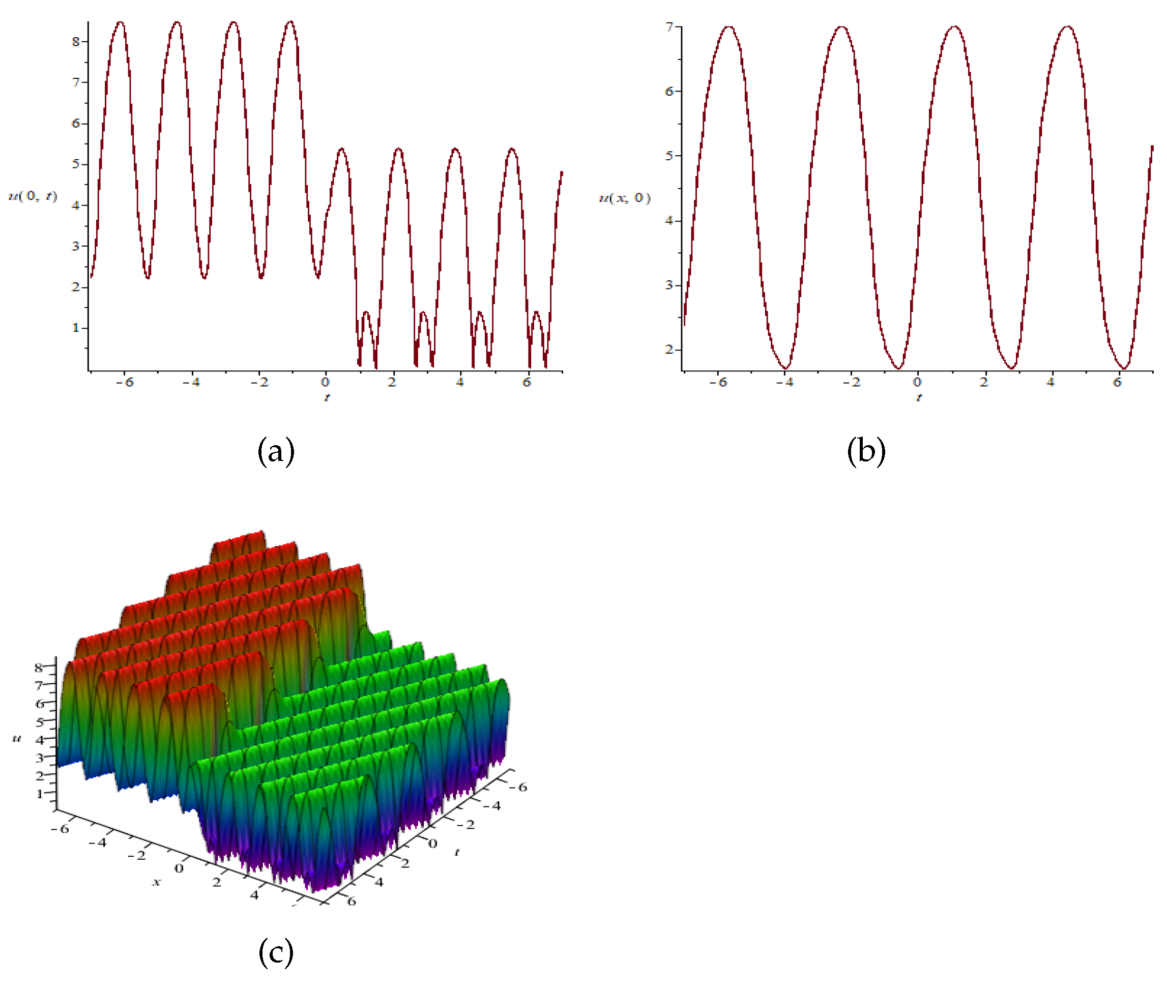
Substituting expressions (49) into (47) and (46), we obtain the exact forms of , , and then we put them into the first two expressions of Equation (45), we will get the exact solutions of u and v. The result is omitted here because of its prolixity, but the corresponding images of u and v are as follows with the parameters {}.
At the same time, we give the numerical solution of u at as follows.
With the help of , we give the numerical analysis of u at . By taking the value of time t at some key points, the result of numerical analysis is almost completely consistent with the two-dimensional graph Figure 1a of the exact solution. From Table 1, we can see that the value of u changes periodically from to , the value at the highest point is approximately 8.34 and the value at the lowest point is approximately 2.21. When , the value of u suddenly becomes smaller, and then it varies periodically. Combining the two-dimensional and three-dimensional graph, we know that the soliton and the periodic wave interact at this moment to form a kink soliton solution, and the collision between soliton and periodic wave is an elastic collision. Namely, the shape of the wave does not change before and after collision.
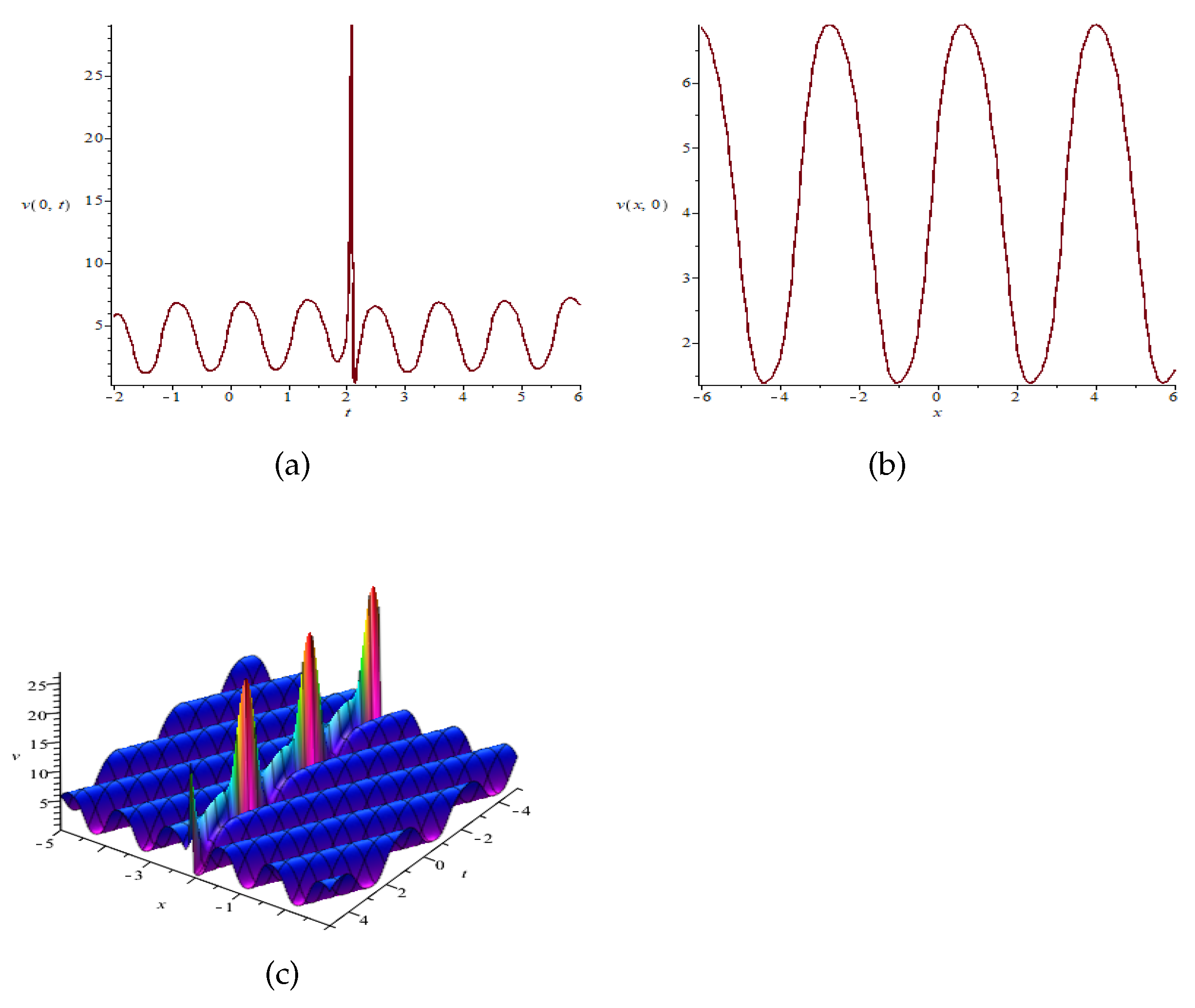
At the same time, we give the numerical solution of v at as follows.
Similar to Table 1, the numerical analysis of v at also be derived. By taking the value of time t at some key points, the numerical analysis is almost completely consistent with the two-dimensional graph Figure 2a of the exact solution. From Table 2, we can see that the value of v reaches the maximum at , which is close to 29.07. That is the result of the interaction between the soliton and the elliptical periodic wave. The collision is an elastic collision. Since, when to 1.2234 and to 5.7031, the values of v present a periodic characteristic, the maximum value is 6.70, and the minimum value is 1.36.
Similarly, we can get the change of u with time t at different positions of x, and the change rule is consistent with that at .
Case 4.
. It leads to the following similarity solutions
where and .
Substituting the expressions (50) into the prolonged system, we derive
and satisfies elliptic equation
with , or
For this subcase, according to the method of subcase 3, one can also get the interaction solutions of u and v, which reflect the interactions between Jacobian elliptic function and rational function.
6. Conclusions and Further Researches
In this paper, we provide the basic method to construct the nonlocal symmetry of nonlinear PDE, employ this method to derive the local and nonlocal symmetries of Equation (1), give the corresponding finite symmetry transformations theorem, and discuss the similarity reductions of the prolonged system. Furthermore, the Painlevé integral property and two types of new exact solutions are presented, which include the special interaction solutions between the soliton and the cnoidal periodic wave, and the soliton with rational function solution. This kind of solution can be easily applicable to the analysis of physically interesting processes. Besides, we also give the numerical analysis of the CKdV equations, which can verify the properties of exact solution.
For the provided method in this paper, we only consider the Lax pairs as the auxiliary system. However, if we choose the Bäcklund transformation, potential system, pseudo-potential as the auxiliary system, maybe, we can obtain different nonlocal symmetries.
Meanwhile, there is an other interesting thing that the CKdV Equation (1) have close relationship with the AB-KdV. If we let (where and are the usual parity and time-reversal operators respectively) and put the above assumption into Equation (1), then (1) will be reduced to the following integrable nonlocal AB-KdV equations
Therefore, for the symmetry reduction 1 and 2, leads to , then we can further deduce and derive the PT (Parity and Time) symmetric exact solution for the AB-KdV equation by the transformations of .
Based on the above facts, we consider whether all of the coupled equations can be reduced to a corresponding nonlocal AB equation. If so, whether we can get some new types of solutions of nonlocal equations by solving the corresponding local equations will be discussed in our future work.
Author Contributions
Investigation, Y.X., R.Y., Y.L., Software & Computing, Y.X., Methodology, X.X., Writing-original draft, Y.X., Analysis, Y.L., Validation, Y.X., Review & editing, R.Y. All authors have read and agreed to the published version of the manuscript.
Funding
The project is supported by the National Natural Science Foundation of China (Grant Nos. 12001424, 11471004), the Natural Science Basic research program of Shaanxi Province (No. 2021JZ-21), The Chinese Post doctoral Science Foundation (No. 2020M673332), Liaocheng University level science and technology research fund (No. 318012018), Research Award Foundation for Outstanding Young Scientists of Shandong Province (No. BS2015SF009), the Fundamental Research Funds for the Central Universities (No. 2020CBLY013).
Institutional Review Board Statement
Not applicable.
Informed Consent Statement
Not applicable.
Conflicts of Interest
The authors declare no conflict of interest.
References
- Lie, S. Sophus Lie’s 1880 Transformation Group Paper; Ackerman, M., Hermann, R., Eds.; Mathematical Sciene Press: Brookline, MA, USA, 1975. [Google Scholar]
- Freire, I.L.; Torrisi, M. Symmetry methods in mathematical modeling of Aedes aegypti dispersal dynamics. Nonlinear Anal-Real 2013, 14, 1300. [Google Scholar] [CrossRef]
- Hussain, A.; Bano, S.; Khan, I.; Baleanu, D.; Nisar, K.S. Lie Symmetry Analysis, Explicit Solutions and Conservation Laws of a Spatially Two-Dimensional Burgers-Huxley Equation. Symmetry 2020, 12, 170. [Google Scholar] [CrossRef] [Green Version]
- Aliyu, A.I.; Inc, M.; Yusuf, A.; Baleanu, D. Symmetry Analysis, Explicit Solutions, and Conservation Laws of a Sixth-Order Nonlinear Ramani Equation. Symmetry 2018, 10, 341. [Google Scholar] [CrossRef] [Green Version]
- Krasil’shchik, I.S.; Vinogradov, A.M. A method of calculating higher symmetries of nonlinear evolutionary equations, and nonlocal symmetries. Dokl. Akad. Nauk SSSR 1980, 253, 1289. [Google Scholar]
- Galas, F. New nonlocal symmetries with pseudopotentials. J. Phys. A Math. Gen. 1992, 25, L981. [Google Scholar] [CrossRef]
- Bluman, G.W.; Cheviakov, A.F.; Anco, S.C. Applications of Symmetry Methods to Partial Differential Equations; Springer: New York, NY, USA, 2010. [Google Scholar]
- Bluman, G.W.; Cheviakov, A.F. Framework for potential systems and nonlocal symmetries: Algorithmic approach. J. Math. Phys. 2005, 46, 123506. [Google Scholar] [CrossRef] [Green Version]
- Euler, N.; Euler, M. On Nonlocal Symmetries, Nonlocal Conseration Laws and Nonlocal Transformations of Evolution Equation: Two linearisable Hierarchies. J. Nonlinear Math. Phys. 2009, 16, 489. [Google Scholar] [CrossRef] [Green Version]
- Euler, M.; Euler, N.; Reyes, E.G. Multipotentializations and nonlocal symmetries: Kupershmidt, Kaup-Kupershmidt and Sawada-Kotera equations. J. Nonlinear Math. Phys. 2017, 24, 303. [Google Scholar] [CrossRef]
- Lou, S.Y.; Hu, X.B. Nonlocal Lie-Bäclund symmetries and Olver symmetries of the KdV equation. Chin. Phys. Lett. 1993, 10, 577. [Google Scholar] [CrossRef]
- Lou, S.Y.; Hu, X.R.; Chen, Y. Nonlocal symmetries related to Bäcklund transformation and their applications. J. Phys A Math. Gen. 2012, 45, 155205. [Google Scholar] [CrossRef] [Green Version]
- Lou, S.Y. Negative Kadomtsev-Petviashvili hierarchy. Phys. Scr. 1998, 57, 481. [Google Scholar] [CrossRef]
- Reyes, E.G. The modified Camassa-Holm equation. Int. Math. Res. Notices 2015, 12, 2617. [Google Scholar]
- Gao, X.N.; Lou, S.Y.; Tang, X.Y. Bosonization, singularity analysis, nonlocal symmetry reductions and exact solutions of supersymmetric KdV equation. J. High Energy Phys. 2013, 5, 029. [Google Scholar] [CrossRef] [Green Version]
- Xin, X.P.; Miao, Q.; Chen, Y. Nonlocal symmetry, optimal systems, and explicit solutions of the mKdV equation. Chin. Phys. B 2014, 23, 010203. [Google Scholar] [CrossRef]
- Miao, Q.; Xin, X.P.; Chen, Y. Nonlocal symmetries and explicit solutions of the AKNS system. Appl. Math. Lett. 2014, 28, 7. [Google Scholar] [CrossRef]
- Ren, B.; Cheng, X.P.; Lin, J. The (2+ 1)-dimensional Konopelchenko-Dubrovsky equation: Nonlocal symmetries and interaction solutions. Nonlinear Dyn. 2016, 86, 1855. [Google Scholar] [CrossRef]
- Huang, L.L.; Chen, Y. Nonlocal symmetry and similarity reductions for a (2 + 1)-dimensional Korteweg-de Vries equation. Nonlinear Dyn. 2018, 92, 221. [Google Scholar] [CrossRef]
- Xia, Y.R.; Xin, X.P.; Zhang, S.L. Residual symmetry, interaction solutions, and conservation laws of the (2+1)-dimensional dispersive long-wave system. Chin. Phys. B 2017, 26, 030202. [Google Scholar] [CrossRef]
- Xia, Y.R.; Xin, X.P.; Zhang, S.L. Nonlinear Self-Adjointness, Conservation Laws and Soliton-Cnoidal Wave Interaction Solutions of (2+1)-dimensional Modified Dispersive Water-Wave System. Commun. Theor. Phys. 2017, 67, 15. [Google Scholar] [CrossRef]
- Xin, X.P.; Liu, H.Z.; Zhang, L.L.; Wang, Z.G. High order nonlocal symmetries and exact interaction solutions of the variable coefficient KdV equation. Appl. Math. Lett. 2019, 88, 132. [Google Scholar] [CrossRef]
- Feng, Y.; Bilige, S.; Wang, X. Diverse exact analytical solutions and novel interaction solutions for the (2+1)-dimensional Ito equation. Phys. Scr. 2020, 95, 095201. [Google Scholar] [CrossRef]
- Kumar, S.; Kumar, A.; Kharbanda, H. Lie symmetry analysis and generalized invariant solutions of (2+1)-dimensional dispersive long wave (DLW) equations. Phys. Scr. 2020, 95, 065207. [Google Scholar] [CrossRef]
- Xin, X.P.; Zhang, L.L.; Xia, Y.R.; Liu, H.Z. Nonlocal symmetries and exact solutions of the (2+1)-dimensional generalized variable coefficient shallow water wave equation. Appl. Math. Lett. 2019, 94, 112. [Google Scholar] [CrossRef] [Green Version]
- Xia, Y.R.; Yao, R.X.; Xin, X.P. Nonlocal symmetries and group invariant solutions for the coupled variable-coefficient Newell-Whitehead system. J. Nonlinear Math. Phys. 2020, 27, 581. [Google Scholar] [CrossRef]
- Lou, S.Y. Alice-Bob systems, symmetry invariant and symmetry breaking soliton solutions. J. Math. Phys. 2018, 59, 083507. [Google Scholar] [CrossRef]
- Gear, J.A.; Grimshaw, R. Weak and srong interactions between interal solitary waves. Stud. Appl. Math. 1984, 70, 235. [Google Scholar] [CrossRef]
- Lou, S.Y.; Tong, B.; Hu, H.C.; Tang, X.Y. CKdV equations derived from two-layer fluids. J. Phys. A Math. Gen. 2006, 39, 513. [Google Scholar] [CrossRef] [Green Version]
- Hirota, R.; Satsuma, J. Soliton solutions of a couple Korteweg-de-Vries equation. Phys. Lett. A 1981, 85, 407. [Google Scholar] [CrossRef]
- Ramani, A.; Dorizzi, B.; Grammaticos, B. Integrability of Hirota-Satsuma equations: Two tests. Phys. Lett. A 1983, 99, 411. [Google Scholar] [CrossRef]
- Xu, M.H.; Jia, M. Exact Solutions, Symmetry Reductions, Painlevé Test and Bäcklund Transformations of A CKdV Equation. Commun. Theor. Phys. 2017, 68, 417. [Google Scholar]
- Parra, H.P.; Cisneros-Ake, L.A. The direct method for multisolitons and two-hump solitons in the Hirota-Satsuma system. Phys. Lett. A 2020, 384, 126471. [Google Scholar] [CrossRef]
- Milovanovic, G.V.; Parmar, R.K.; Rathie, A.K. Certain Laplace transforms of convolution type integrals involving product of two special pFp functions. Demonstr. Math. 2018, 51, 264. [Google Scholar] [CrossRef]
- Fitri, S.; Marjono, M.; Thomas, D.K.; Wibowo, R.B.E. Coefficient inequalities for a subclass of Bazilevic functions. Demonstr. Math. 2020, 53, 27. [Google Scholar] [CrossRef]
- Kumar, H.; Kumar, A.; Ch, F.; Singh, R.M.; Gautam, M.S. Construction of new traveling and solitary wave solutions of a nonlinear PDE characterizing the nonlinear low-pass electrical transmission lines. Phys. Scr. 2021, 96, 085215. [Google Scholar] [CrossRef]
- Riaz, M.B.; Atangana, A.; Jhangeer, A.; Rehman, M.J.U. Some exact explicit solutions and conservation laws of Chaffee-Infante equation by Lie symmetry analysis. Phys. Scr. 2021, 96, 084008. [Google Scholar] [CrossRef]
- Shen, Y.; Tian, B.; Liu, S.H.; Yang, D.Y. Bilinear Bäcklund transformation, soliton and breather solutions for a (3+1)-dimensional generalized Kadomtsev-Petviashvili equation in fluid dynamics and plasma physics. Phys. Scr. 2021, 96, 075212. [Google Scholar] [CrossRef]
- Fokou, M.; Kofane, T.C.; Mohamadou, A.; Yomba, E. Lump periodic wave, soliton periodic wave, and breather periodic wave solutions for third-order (2+1)-dimensional equation. Phys. Scr. 2021, 96, 055223. [Google Scholar] [CrossRef]
- Ablowitz, M.J.; Ramani, A.; Segur, H. A connection between nonlinear evolution equations and ordinary differential equations of P-type.I. J. Math. Phys. 1980, 21, 715. [Google Scholar] [CrossRef]
Figure 1.
The kink soliton+cnoidal periodic wave solution for u. (a) The profile of the special structure with . (b) The profile of the special structure with . (c) The 3D soliton-cnodial periodic wave interaction solution to u.
Figure 1.
The kink soliton+cnoidal periodic wave solution for u. (a) The profile of the special structure with . (b) The profile of the special structure with . (c) The 3D soliton-cnodial periodic wave interaction solution to u.

Figure 2.
The bright soliton+cnoidal periodic wave solution for v. (a) The profile of the special structure with , (b) The profile of the special structure with , (c) The 3D soliton-cnodial periodic wave interaction solution to v.
Figure 2.
The bright soliton+cnoidal periodic wave solution for v. (a) The profile of the special structure with , (b) The profile of the special structure with , (c) The 3D soliton-cnodial periodic wave interaction solution to v.


Table 1.
Numerical analysis of u at .
| x | 0 | 0 | 0 | 0 | 0 | 0 | 0 | 0 | 0 |
|---|---|---|---|---|---|---|---|---|---|
| t | −7 | −6.2354 | −6 | −5.2777 | −4 | −3.5919 | −2.8640 | −2 | −1.9063 |
| u | 2.21334 | 8.33976 | 8.31707 | 2.21344 | 5.06270 | 2.21352 | 8.33954 | 2.38391 | 2.21331 |
| x | 0 | 0 | 0 | 0 | 0 | 0 | 0 | 0 | 0 |
| t | −1.1783 | −1 | −0.2516 | 0.5049 | 1 | 1.2401 | 1.4742 | 2 | 2.1255 |
| u | 8.33943 | 8.45273 | 2.21235 | 5.35937 | 0.01779 | 1.3420 | 0.017117 | 5.07370 | 5.35921 |
| x | 0 | 0 | 0 | 0 | 0 | 0 | 0 | 0 | 0 |
| t | 2.6881 | 2.9258 | 3 | 3.1599 | 3.8113 | 4 | 4.3715 | 4.5250 | 4.8492 |
| u | 0.01816 | 1.34208 | 1.10875 | 0.01761 | 5.35924 | 5.02672 | 0.01780 | 1.34188 | 0.01737 |
| x | 0 | 0 | 0 | 0 | 0 | 0 | 0 | 0 | 0 |
| t | 5 | 5.4971 | 6 | 6.0573 | 6.3030 | 6.5315 | |||
| u | 1.82085 | 5.35929 | 0.98980 | 0.01704 | 1.33029 | 0.01664 |
Table 2.
Numerical analysis of v at .
| x | 0 | 0 | 0 | 0 | 0 | 0 | 0 | 0 | 0 |
|---|---|---|---|---|---|---|---|---|---|
| t | −2 | −2.0035 | −1.5320 | −1 | −0.9694 | −0.3412 | 0.3051 | 0.7705 | 1 |
| u | 5.59065 | 5.54969 | 1.35679 | 6.55527 | 6.69761 | 1.35605 | 6.69981 | 1.46356 | 2.96166 |
| x | 0 | 0 | 0 | 0 | 0 | 0 | 0 | 0 | 0 |
| t | 1.2234 | 1.8534 | 2 | 2.0883 | 2.1418 | 2.4900 | 2.9770 | 3 | 3.6751 |
| u | 6.69693 | 2.09575 | 4.69652 | 29.07161 | 0.039392 | 6.53238 | 1.35676 | 1.28513 | 6.64508 |
| x | 0 | 0 | 0 | 0 | 0 | 0 | 0 | 0 | 0 |
| t | 4 | 4.1479 | 4.6155 | 5 | 5.2619 | 5.7031 | |||
| u | 2.45604 | 1.38254 | 6.69679 | 4.68181 | 1.50911 | 6.69698 |
Publisher’s Note: MDPI stays neutral with regard to jurisdictional claims in published maps and institutional affiliations. |
© 2021 by the authors. Licensee MDPI, Basel, Switzerland. This article is an open access article distributed under the terms and conditions of the Creative Commons Attribution (CC BY) license (https://creativecommons.org/licenses/by/4.0/).
Share and Cite
MDPI and ACS Style
Xia, Y.; Yao, R.; Xin, X.; Li, Y. Nonlocal Symmetry, Painlevé Integrable and Interaction Solutions for CKdV Equations. Symmetry 2021, 13, 1268. https://0-doi-org.brum.beds.ac.uk/10.3390/sym13071268
AMA Style
Xia Y, Yao R, Xin X, Li Y. Nonlocal Symmetry, Painlevé Integrable and Interaction Solutions for CKdV Equations. Symmetry. 2021; 13(7):1268. https://0-doi-org.brum.beds.ac.uk/10.3390/sym13071268
Chicago/Turabian StyleXia, Yarong, Ruoxia Yao, Xiangpeng Xin, and Yan Li. 2021. "Nonlocal Symmetry, Painlevé Integrable and Interaction Solutions for CKdV Equations" Symmetry 13, no. 7: 1268. https://0-doi-org.brum.beds.ac.uk/10.3390/sym13071268
Note that from the first issue of 2016, this journal uses article numbers instead of page numbers. See further details here.