Symmetries and Related Physical Balances for Discontinuous Flow Phenomena within the Framework of Lagrange Formalism

Abstract

By rigorous analysis, it is proven that from discontinuous Lagrangians, which are invariant with respect to the Galilean group, Rankine–Hugoniot conditions for propagating discontinuities can be derived via a straight forward procedure that can be considered an extension of Noether’s theorem. The use of this general procedure is demonstrated in particular for a Lagrangian for viscous flow, reproducing the well known Rankine–Hugoniot conditions for shock waves.

1. Introduction

The formulation of physical theories within the framework of variational principles enables a deeper understanding of the physical system in many respects [1]. In particular, the symmetries of the Lagrangian and their relation to physical conservation laws, which was established via Noether’s theorem [2], is a good example for it. In the classical theory of Lagrangian formalism, one usually assumes two-times continuously differentiable fields, but fluid dynamics also includes discontinuous phenomena, such as shock waves, for whose description one uses transition conditions at the shock front—so-called Rankine–Hugoniot conditions [3,4,5]. Analogous conditions are also used in fracture mechanics [6]. Although such considerations are outside the Lagrangian formalism, the Rankine–Hugoniot conditions are essentially based on conservation of physical quantities, such as mass, momentum and energy. This poses the question of whether there is a way to obtain such conditions via Noether’s theorem, applied to fundamental symmetries of the Lagrangian and, in particular, the Galilean group.

In the present context, some prior works serve as starting points for our investigations, beginning with the classical Lagrangian for inviscid flows proposed by Seliger and Witham [7] and the rigorous analysis undertaken by Scholle [8], which delivers general rules that have to be followed in the formulation of Lagrangians to ensure Galilean invariance. By utilizing the rules formulated in [8] in order to extend the Lagrangian proposed in Seliger and Witham [7] toward viscous flow, Scholle and Marner [9] obtained an extended Lagrangian for viscous flows, which, in the special case of vanishing shear viscosity but nonzero volume viscosity, reproduces the Lagrangian proposed by Zuckerwar and Ash [10] a few years before. By considering some flow examples of prototypic character, however, partly unphysical solutions were obtained in [9], showing the necessity for further modifications of the Lagrangian. In order to resolve the above issue, Scholle and Marner [9] followed an idea of Anthony [11,12,13], who suggested a complex field $\chi$ of thermal excitation, serving as an analogue to Schrödinger’s matter field. A brief summary of Anthony’s concept, which was originally motivated by an analogy between quantum mechanics and fluid mechanics discovered by Madelung [14], is provided in the appendix of the recent work [15]. On introduction of the complex field $\chi$, a discontinuity is imposed in the resulting Lagrangian, which goes beyond the usual framework in continuum theory so that from the variation with respect to the fundamental fields, in addition to the well-known Euler–Lagrange equations, corresponding transition and production conditions along the discontinuity surfaces result. Furthermore, an additional parameter ${\omega }_0$ becomes relevant. This surprising result can be interpreted against the background that the physical phenomenon viscosity weakly violates both the thermodynamic equilibrium and the continuum hypothesis, which leads to the occurrence of discontinuities in the sense of microscopic fluctuations, where ${\omega }_0$ serves as a thermodynamic relaxation rate. Consequently, in the limiting case ${\omega }_0\to \infty$, the classical Navier–Stokes theory is reproduced.

Although the focus of [9] was the reproduction of the classical Navier–Stokes theory from an unconventional Lagrangian, subsequent papers [15,16,17] showed a further development in the direction of linear and weakly nonlinear acoustics; in the outlook of the paper [9], the possibility of applying the general formalism also to discontinuous phenomena on a macroscopic scale, including shock waves, is pointed out. Therefore, the aim of the present paper is to address this yet unresolved issue and to derive the Rankine–Hugoniot conditions from the symmetries of the Lagrangian, which, at first, requires the mathematical derivation of an extended Noether theorem, considering discontinuities. In a second step, the general theory is applied to viscous flow theory. Both were not performed in the prior work [9].

This paper is structured as follows: in Section 2, the general theory is presented, starting with a review on Hamilton’s principle (Section 2.1), followed by a detailed analysis about the Galilean group and its manifestation with regard to the respective Lagrangian (Section 2.2) and the balances resulting from Noether’s theorem (Section 2.3). In Section 2.4, it is demonstrated that transition and production conditions are obtained from discontinuous Lagrangians. Finally, in Section 2.5, the desired Rankine–Hugoniot conditions for Noether fluxes are derived. In Section 3, the procedure is applied to shock waves. A discussion of the results is provided in Section 4.

2. General Theory

2.1. Hamilton’s Principle and Euler–Lagrange Equations

The evolution of a material continuum between initial time $t_1$ and final time $t_2$ is given by Hamilton’s principle, i.e., by free and independent variation $\delta I=0$ of the action integral as follows:

$$I=\underset{t_1}{\overset{t_2}{\int }}\underset{V\left(t\right)}{\int \int \int }\ell \left({\psi }_i,{\dot{\psi }}_i,\nabla {\psi }_i\right)\mathrm{d}V\mathrm{d}t,$$

(1)

with respect to a set of N fundamental fields ${\psi }_1,\cdots ,{\psi }_N$, where initial and final state are fixed. $V=V\left(t\right)$ denotes the volume of the system. The Lagrangian

$$\ell =\ell \left({\psi }_i,{\dot{\psi }}_i,\nabla {\psi }_i\right)$$

(2)

is a function of the fields, their first order time derivatives ${\dot{\psi }}_i=\partial {\psi }_i/\partial t$, and their gradients $\nabla {\psi }_i$.

Hamilton’s principle implies the set of N basic field equations as follows:

$$\frac{\partial \ell }{\partial {\psi }_i}-\frac{\partial }{\partial t}\left(\frac{\partial \ell }{\partial \dot{{\psi }_i}}\right)-\nabla ·\left(\frac{\partial \ell }{\partial \nabla {\psi }_i}\right)=0,i=1,\cdots ,N,$$

(3)

the so-called Euler–Lagrange equations [1].

2.2. Galilean Invariance and Implications for the Lagrangian

If a system is physically closed, i.e., isolated from the surrounding, its equations of motion are invariant with respect to the following four universal symmetry transformations of the Galilean group, corresponding to the homogeneity of time and space, isotropy of space and equality of all inertial frames:

• time translations:

  $$t\to t^{\prime }=t+\tau$$

  (4)
• space translations:

  $$\overrightarrow{x}\to {\overrightarrow{x}}^{\prime }=\overrightarrow{x}+\overrightarrow{s}$$

  (5)
• rigid rotations:

  $$\overrightarrow{x}\to {\overrightarrow{x}}^{\prime }=\underline{\mathrm{R}}\overrightarrow{x}$$

  (6)
• Galilei boosts:

  $$\overrightarrow{x}\to {\overrightarrow{x}}^{\prime }=\overrightarrow{x}-{\overrightarrow{u}}_{0}t$$

  (7)

Here, the scalar $\tau$, the two vectors $\overrightarrow{s}$ and ${\overrightarrow{u}}_0$ and the unitary matrix $\underline{\mathrm{R}}$ fulfilling ${\underline{\mathrm{R}}}^T\underline{\mathrm{R}}=\underline{I}$ and $det\underline{\mathrm{R}}=1$ are constants. Here, and in the following, an underbar denotes a matrix/tensor and $\underline{I}$ is the unity matrix/tensor. Via formulae (4)–(7), the four symmetries are obviously well-defined for discrete systems, for instance, systems of point masses in Newtonian mechanics. For continuous systems, the situation is essentially different: in field theories, the formulae (4)–(7) have to be supplemented by the respective transformation formulae for the fields in order to define the transformations completely.

Through a rigorous analysis, Scholle [8] showed that Galilean invariance imposes constraints on the analytic form of the Lagrangian density. A basic finding is the existence of two different but equivalent representations of each Galilei-invariant Lagrangian: for each Lagrangian of the form (2), subsequently called the conventional representation, which is invariant w.r.t. all transformations (4)–(7) of the Galilei group, the following transformation exists:

$$\begin{array}{cc}\hfill {\psi }_i& =K_i\left({\Psi }_j,\zeta ,\nabla \zeta \right),\hfill \end{array}$$

(8)

$$\begin{array}{cc}\hfill \zeta & :=\frac{{\overrightarrow{x}}^2}{2t}\hfill \end{array}$$

(9)

defining a different set of fundamental fields ${\Psi }_j$ and turning the Lagrangian (2) to a different form as follows:

$$\begin{array}{cc}\hfill \ell \left(K_i\left({\Psi }_j,\zeta ,\nabla \zeta \right),{\dot{K}}_i\left({\Psi }_j,\zeta ,\nabla \zeta \right),\nabla K_i\left({\Psi }_j,\zeta ,\nabla \zeta \right)\right)& =\ell \left({\Psi }_i,\stackrel{\circ }{{\Psi }_i},\nabla {\Psi }_i+\frac{1}{t}{\overrightarrow{K}}_i\left({\Psi }_j\right)\right),\hfill \end{array}$$

(10)

$$\begin{array}{cc}\hfill {\overrightarrow{K}}_i\left({\Psi }_j\right)& :=\underset{\zeta ,\nabla \zeta \to 0}{lim}\frac{\partial K_i}{\partial (\nabla \zeta )},\hfill \end{array}$$

(11)

where the ring symbol $\stackrel{\circ }{}$ indicates the dual time derivative [8]:

$${\stackrel{\circ }{\Psi }}_j:=\left\{\frac{\partial }{\partial t}+\nabla \zeta ·\nabla \right\}{\Psi }_j,$$

(12)

which, in contrast to the conventional time derivative, is invariant w.r.t. Galilei boosts. $\zeta$ is called the generating field. As a consequence, the Lagrangian in its alternative form $\ell \left({\Psi }_i,\stackrel{\circ }{{\Psi }_i},\nabla {\Psi }_i+{\overrightarrow{K}}_i\left({\Psi }_j\right)/t\right)$, subsequently called the dual representation, proves to be invariant with respect to Galilei boosts if all fields ${\psi }_i$ are assumed to be likewise invariant. Thus, the essence of the dual representation is that Galilei boosts become manifest as pure geometrical transformations without the need to combine them with a re-gauging of potentials [18]. Since the conventional representation $\ell \left({\psi }_i,{\dot{\psi }}_i,\nabla {\psi }_i\right)$ is obviously strictly invariant w.r.t. space and time translations while the dual representation is strictly invariant w.r.t. Galilei boosts, simultaneous invariance with respect to translations and Galilei boosts is granted by (10), which consequentially can be understood as a collective symmetry criterion for the Galilean group. It has to be fulfilled by any Lagrangian related to a physically closed continuous system.

Once the functions $K_i$ of the transformation (8) are determined by the collective symmetry criterion (10), the following gauge transformation is well-defined:

$${\psi }_i\to {{\psi }_i}^{\prime }=K_i\left({\psi }_j,\epsilon ,0\right)$$

(13)

and, according to [8], likewise, is a symmetry transformation of the Lagrangian. This induced gauge symmetry is remarkable since it is an indirect but compelling consequence of the Galilean invariance and, therefore, on the same level as all symmetry transformations of the Galilei group, and is consequently to be understood as universal symmetry just like the latter, applied on any physical continuum. Since the parameter $\epsilon$ in (13) may take arbitrary values, the induced gauge symmetry is a one-parameter Lie group.

The mere existence of this symmetry entails further consequences: one of them is the statement that among the N fundamental fields ${\psi }_i$, there must be at least one non-observable one, i.e., a potential field that is non-unique since it is influenced by the gauge transformation (13) and cannot, therefore, be determined by any kind of physical measurement (For the example considered in Section 3, this applies to the Clebsch variable $\xi$). This is proven in [8] by representing the induced gauge transformation as a combination of space translations (5) and Galilei boosts (7).

Further consequences of the invariance w.r.t. the Galilei group, especially regarding the representation of the velocity field by means of potentials, are reported in the review article [18].

2.3. Associated Balances Resulting from Noether’s Theorem

The above-mentioned general properties of Lagrangians in continuum theory entail additional general implications for the physical balances resulting from the variational principle by utilizing Noether’s theorem, the essence of which is that each Lie symmetry of the Lagrangian gives rise to a physical balance equation and to a canonical definition of the density and flux density involved.

All transformations (4)–(7) of the Galilei group are Lie groups; each of them are related to a continuous parameter $\epsilon$. The infinitesimal generators of the group read as follows:

$$\begin{array}{c}\hfill \widehat{t}:={\left.\frac{\partial t^{\prime }}{\partial \epsilon }\right|}_{\epsilon =0},\end{array}$$

(14)

$$\begin{array}{c}\hfill \widehat{\overrightarrow{x}}:={\left.\frac{\partial {\overrightarrow{x}}^{\prime }}{\partial \epsilon }\right|}_{\epsilon =0},\end{array}$$

(15)

$$\begin{array}{c}\hfill {\widehat{\psi }}_i:={\left.\frac{\partial {{\psi }_i}^{\prime }}{\partial \epsilon }\right|}_{\epsilon =0}.\end{array}$$

(16)

Then, Noether’s theorem [2,19,20] gives rise to the definition of a density ${\varrho }_Q$ and an associated flux density${\overrightarrow{j}}_Q$ as follows:

$$\begin{array}{cc}\hfill {\varrho }_Q& :=\ell \widehat{t}+\frac{\partial \ell }{\partial {\dot{\psi }}_i}\left[{\widehat{\psi }}_i-{\dot{\psi }}_i\widehat{t}-\widehat{\overrightarrow{x}}·\nabla {\psi }_i\right],\hfill \end{array}$$

(17)

$$\begin{array}{cc}\hfill {\overrightarrow{j}}_Q& :=\ell \widehat{\overrightarrow{x}}+\frac{\partial \ell }{\partial \nabla {\psi }_i}\left[{\widehat{\psi }}_i-{\dot{\psi }}_i\widehat{t}-\widehat{\overrightarrow{x}}·\nabla {\psi }_i\right],\hfill \end{array}$$

(18)

fulfilling the homogeneous balance equation as follows:

$$\frac{\partial {\varrho }_Q}{\partial t}+\nabla ·{\overrightarrow{j}}_Q=0.$$

(19)

In Equations (17) and (18), subsequently, the following Einstein notation is utilized: an index variable appearing twice in a single term implies summation of that term over all values of the index.

Physically, Equation (19) is associated with the conservation of the global quantity as follows:

$$Q:=\underset{V}{\int }{\varrho }_Q\mathrm{d}V$$

(20)

with V being the entire volume of the continuum. More generally, if a Lie group with m continuous parameters ${\epsilon }_1,\cdots ,{\epsilon }_m$ is considered, for each parameter, a balance equation of the type (19) is obtained.

In

Table 1. Relations between symmetries and balances resulting from Noether’s theorem.

Symmetry	$\widehat{\mathit{t}}$	$\widehat{\overrightarrow{\mathit{x}}}$	${\widehat{\mathit{\psi }}}_{\mathit{i}}$	Balance	Density	Flux Density
time transl.	1	0	0	energy	$w=\frac{\partial \ell }{\partial \dot{{\psi }_i}}\dot{{\psi }_i}-\ell$	$\overrightarrow{S}=\frac{\partial \ell }{\partial \nabla {\psi }_i}\dot{{\psi }_i}$
space transl.	0	$\underline{1}$	0	momentum	$\overrightarrow{p}=-\frac{\partial \ell }{\partial \dot{{\psi }_i}}\nabla {\psi }_i$	$\underline{\Pi }=\ell \underline{1}-\frac{\partial \ell }{\partial \nabla {\psi }_i}\otimes \nabla {\psi }_i$
ind. gauge	0	0	$K_{0i}$	mass	$\varrho =-\frac{\partial \ell }{\partial \dot{{\psi }_i}}{K}_{0i}\left({\psi }_j\right)$	$\varrho \overrightarrow{u}=-\frac{\partial \ell }{\partial \nabla {\psi }_i}{K}_{0i}\left({\psi }_j\right)$

, the infinitesimal generators for time/space translations and the induced gauge symmetry, the associated global quantities, related densities and flux densities are listed, with the infinitesimal generator $K_{0i}\left({\psi }_j\right)$ defined as follows:

$$K_{0i}\left({\psi }_j\right):=\underset{\zeta ,\nabla \zeta \to 0}{lim}\frac{\partial K_i}{\partial \zeta }.$$

(21)

The Noether balance associated with rigid rotations (6) is the angular momentum balance, which is not discussed in this paper. Finally, the Noether balance associated with Galilei boosts (7) is analyzed by considering the dual representation (10) of the Lagrangian in terms of the fields ${\Psi }_j$ being invariant w.r.t. (7). Thus, the associated density and flux density read as follows:

$$\begin{array}{cc}\hfill \overrightarrow{z}& =t\frac{\partial \ell }{\partial {\dot{\Psi }}_j}\nabla {\Psi }_j,\hfill \end{array}$$

(22)

$$\begin{array}{cc}\hfill \underline{Z}& :=-t\ell \underline{1}+t\frac{\partial \ell }{\partial \nabla {\Psi }_j}\otimes \nabla {\Psi }_j,\hfill \end{array}$$

(23)

and the associated Noether balance

$$\frac{\partial \overrightarrow{z}}{\partial t}+\nabla ·\underline{Z}=0,$$

(24)

is related to the motion of the system’s center of mass; see, for example, [21]. The physical significance of the density $\overrightarrow{z}$ and the flux density $\underline{Z}$ becomes clearer by transforming the Noether expressions according to (8) back into conventional representation, revealing the following constitutive relations:

$$\begin{array}{cc}\hfill \overrightarrow{z}& =\varrho \overrightarrow{x}-\overrightarrow{p}t\stackrel{=:{\overrightarrow{z}}^{*}}{\overbrace{-\frac{\partial \ell }{\partial \dot{{\psi }_i}}{\overrightarrow{K}}_i\left({\psi }_j\right)}},\hfill \end{array}$$

(25)

$$\begin{array}{cc}\hfill \underline{Z}& =\varrho \overrightarrow{u}\otimes \overrightarrow{x}-\underline{\Pi }t\underset{=:{\underline{Z}}^{*}}{\underbrace{-\frac{\partial \ell }{\partial \nabla {\psi }_i}{\overrightarrow{K}}_i\left({\psi }_j\right)}},\hfill \end{array}$$

(26)

showing in particular how the density $\overrightarrow{z}$ and the flux density $\underline{Z}$ are related to the mass density, the mass flux density $\varrho \overrightarrow{u}$, the momentum density $\overrightarrow{p}$, the momentum flux density $\underline{\Pi }$ and additional contributions ${\overrightarrow{z}}^{*}$ and ${\underline{Z}}^{*}$, the physical meaning of which is revealed subsequently: considering the mass and momentum balance, Equation (24) simplifies to the following form:

$$\begin{array}{cc}\hfill 0& =\frac{\partial \overrightarrow{z}}{\partial t}+\nabla ·\underline{Z}\hfill \\ \hfill & =\underset{0}{\underbrace{\left[\frac{\partial \varrho }{\partial t}+\nabla ·\left(\varrho \overrightarrow{u}\right)\right]}}\overrightarrow{x}+\varrho \overrightarrow{u}-\underset{0}{\underbrace{\left[\frac{\partial \overrightarrow{p}}{\partial t}+\nabla ·\underline{\Pi }\right]}}t-\overrightarrow{p}+\frac{\partial {\overrightarrow{z}}^{*}}{\partial t}+\nabla ·{\underline{Z}}^{*},\hfill \end{array}$$

revealing a fundamental relation between mass flux density and momentum flux density:

$${\overrightarrow{p}}^{*}:=\overrightarrow{p}-\varrho \overrightarrow{u}=\frac{\partial {\overrightarrow{z}}^{*}}{\partial t}+\nabla ·{\underline{Z}}^{*},$$

(27)

Note that in classical continuum mechanics, the mass flux density and the momentum density are expected to be equal. However, as can be seen from Equation (27), this is not mandatory: the difference between both, ${\overrightarrow{p}}^{*}:=\overrightarrow{p}-\varrho \overrightarrow{u}$, is called the quasi-momentum density and can be interpreted as contributions to the momentum due to non-material degrees of freedom, e.g., electromagnetic fields, thermal fields and also due to phenomena beyond the scope of continuum theories on a molecular scale, e.g., Brownian motion. Regarding the latter, Fruleux et al. [22] investigated in these additional contribution to the momentum caused by Brownian motion for non-equilibrium case, which they termed a “momentum transfer deficit”, in detail. In [9], the role of Brownian motion for viscosity is emphasized. Despite the fact that within the framework of continuum theories atoms or molecules are not considered, it is possible to take their disorder on a microscopic scale and the quasi-momentum caused by the latter into account by additional fields, here by the three quantities marked with an asterisk, ${\overrightarrow{z}}^{*}$, ${\underline{Z}}^{*}$ and ${\overrightarrow{p}}^{*}$—the displacement density, its associated current density and the quasi-momentum density.

2.4. Variation with a Discontinuous Lagrangian

We now consider a Lagrangian ℓ being discontinuous with respect to the field $\phi ={\psi }_N$ at fixed values ${\phi }_n,n=1,\cdots ,N_S$, but continuously differentiable with respect to all other fields, ${\psi }_i$ with $i<N$, and also continuously differentiable with respect to all derivatives of any field, including $\dot{\phi }$ and $\nabla \phi$. In three-dimensional space, the discontinuities with respect to $\phi$ become manifest along surfaces $S_n\left(t\right)$ defined by: $S_n:=\left\{\overrightarrow{x}|\phi (\overrightarrow{x},t)={\phi }_n\right\}$, $n=1,\cdots ,N_S$, intersecting the system’s volume V into a finite number $N_S+1$ of sub–volumes according to the following:

$$V=\sum _{n=0}^{N_S}{V}_n,$$

(28)

where the sub-volume $V_n$ denotes the region between $S_n$ and $S_{n+1}$ apart from $V_0$ and $V_{N_S}$, denoting the region between the system’s boundary $\partial V$ and $S_1$ or $S_{N_S}$, respectively.

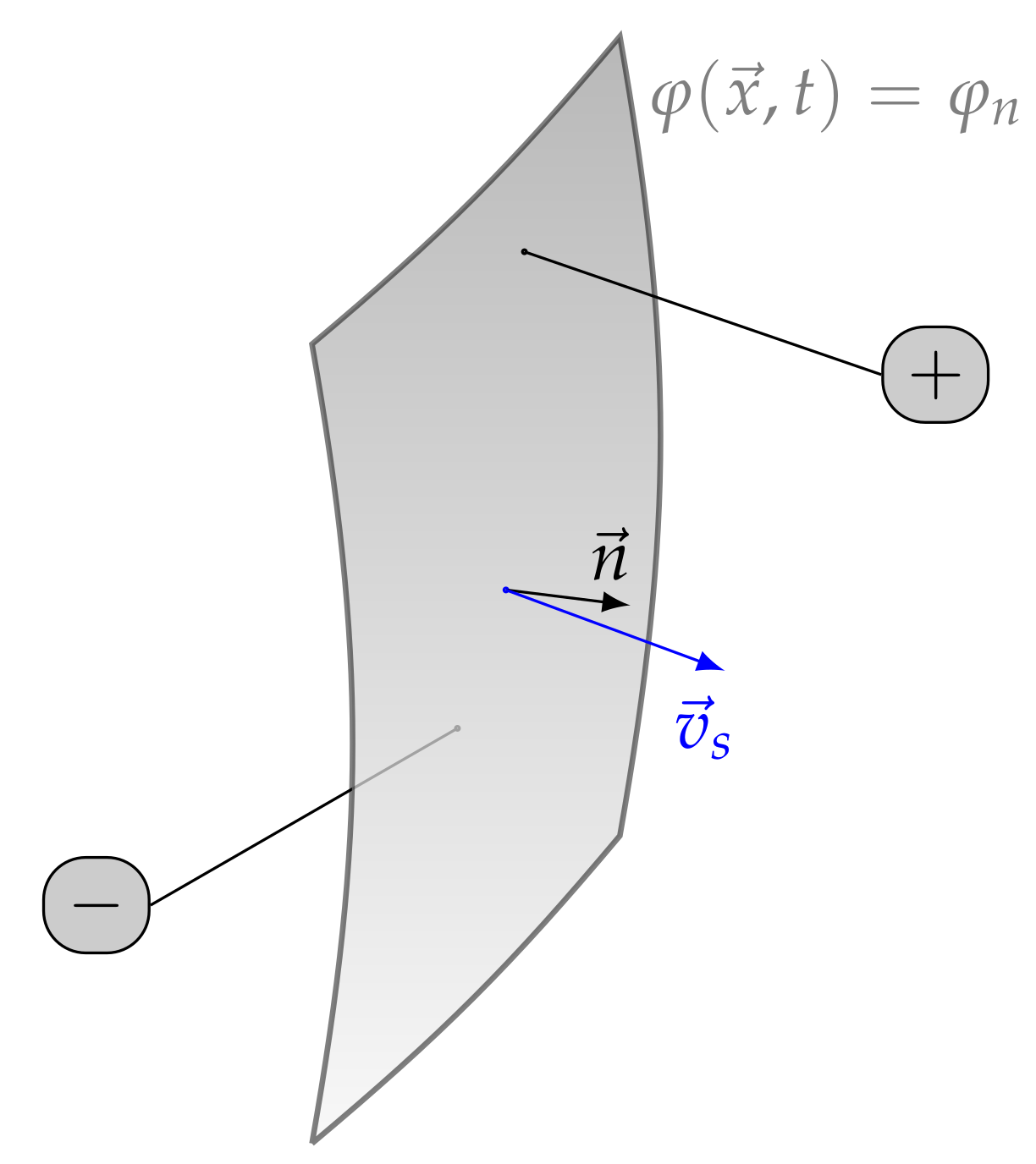
From the physical viewpoint, these time-dependent interfaces, $S_n$, may be related to any kind of discontinuous phenomena like phase boundaries between non-mixable fluids, propagating shock fronts in gaseous media or flame fronts. By

$$\overrightarrow{n}:=\frac{\nabla \phi }{\left|\nabla \phi \right|}$$

(29)

the normal vector of the interface is defined and its local propagation velocity ${\overrightarrow{v}}_s$ is implicitly defined via the following:

$$\frac{\partial \phi }{\partial t}+{\overrightarrow{v}}_s·\nabla \phi =0.$$

(30)

The above vectors are sketched in relation to the discontinuous interface in Figure 1.

By a rigorous analysis, Scholle and Marner [9] showed that variation $\delta I=0$ of the action integral implies the following:

$$\overrightarrow{n}·⟦\frac{\partial \ell }{\partial \nabla {\psi }_i}-{\overrightarrow{v}}_s\frac{\partial \ell }{\partial {\dot{\psi }}_i}⟧=\frac{⟦,\ell ,⟧}{\left|\nabla \phi \right|}{\delta }_{iN},$$

(31)

as matching conditions ($i=1,\cdots ,N-1$) and production conditions ($i=N$) for the generalized fluxes at each interface. The double square bracket indicates the jump at the interface: $⟦\cdots ⟧:={\left[\cdots \right]}_{-}-{\left[\cdots \right]}_{+}$, where ${[\cdots ]}_{\pm }$ indicates the limit of the respective discontinuous expression by approaching it from the front side (subscript +) or the back side (subscript −) of the interface $S_n$.

Independent of the formal proof given above, the matching conditions (for $i=1,\cdots ,N-1$) can also be understood as natural boundary conditions at the phase boundaries in a multiphase flow when assuming that all phases of the flow consist of the same liquid, leading to the same Equation (31).

2.5. Rankine–Hugoniot Conditions for Canonical Noether Fluxes

We consider the Noether flux from the viewpoint of an observer moving alongside with the discontinuity interface $S_n$, ${\overrightarrow{j}}_Q-{\varrho }_Q{\overrightarrow{v}}_s$ and evaluate its contribution to a flux across the discontinuity interface by taking the normal component, $\overrightarrow{n}·\left[{\overrightarrow{j}}_Q-{\varrho }_Q{\overrightarrow{v}}_s\right]$. Then, conservation of the related global quantity Q depends significantly on whether the flux across the discontinuity surface remains continuous or not. Thus, one has to compute the following:

$$\begin{array}{cc}\hfill \overrightarrow{n}·⟦{\overrightarrow{j}}_Q-{\varrho }_Q{\overrightarrow{v}}_s⟧& =\overrightarrow{n}·⟦\left(\widehat{\overrightarrow{x}}-{\overrightarrow{v}}_s\widehat{t}\right)\ell +\left(\frac{\partial \ell }{\partial \nabla {\psi }_i}-{\overrightarrow{v}}_s\frac{\partial \ell }{\partial {\dot{\psi }}_i}\right)\left({\widehat{\psi }}_i-{\dot{\psi }}_i\widehat{t}-\widehat{\overrightarrow{x}}·\nabla {\psi }_i\right)⟧\hfill \\ \hfill & =\overrightarrow{n}·\left(\widehat{\overrightarrow{x}}-{\overrightarrow{v}}_s\widehat{t}\right)⟦\ell ⟧+\overrightarrow{n}·⟦\frac{\partial \ell }{\partial \nabla {\psi }_i}-{\overrightarrow{v}}_s\frac{\partial \ell }{\partial {\dot{\psi }}_i}⟧\left({\widehat{\psi }}_i-{\dot{\psi }}_i\widehat{t}-\widehat{\overrightarrow{x}}·\nabla {\psi }_i\right)\hfill \end{array}$$

(32)

By considering the matching and production conditions (31), the definition (29) and the identity (30), Equation (32) simplifies to the following:

$$\overrightarrow{n}·⟦{\overrightarrow{j}}_Q-{\varrho }_Q{\overrightarrow{v}}_s⟧=\overrightarrow{n}·\left(\widehat{\overrightarrow{x}}-{\overrightarrow{v}}_s\widehat{t}\right)⟦\ell ⟧+\frac{⟦\ell ⟧}{\left|\nabla \phi \right|}\left(\widehat{\phi }-\dot{\phi }\widehat{t}-\widehat{\overrightarrow{x}}·\nabla \phi \right)=⟦\ell ⟧\frac{\widehat{\phi }}{\left|\nabla \phi \right|}$$

and therefore to the desired Rankine–Hugoniot condition:

$$\overrightarrow{n}·⟦{\overrightarrow{j}}_Q-{\varrho }_Q{\overrightarrow{v}}_s⟧=\widehat{\phi }\frac{⟦\ell ⟧}{\left|\nabla \phi \right|}$$

(33)

for the flux of the associated quantity Q across the interface.

Thus, an extension of Noether’s theorem to systems with discontinuities is achieved, which, like the corresponding balance Equation (19) for continuous systems, accounts for the conservation of the respective observable Q at the interface, provided that the infinitesimal generator $\widehat{\phi }$ vanishes. This is the case for all symmetries of the Galilei group and for the induced gauge symmetry, as demonstrated below.

2.5.1. Energy

In the case of the time translation (4) with again ${\widehat{\psi }}_i=0$, the associated Rankine–Hugoniot condition (33) for the energy flux reads as follows:

$$\overrightarrow{n}·⟦\overrightarrow{S}-w{\overrightarrow{v}}_s⟧=0$$

(34)

2.5.2. Momentum

From the space translation (5) with ${\widehat{\psi }}_i=0$, one receives via (33) the Rankine–Hugoniot condition for the momentum flux as follows:

$$\overrightarrow{n}·⟦\underline{\Pi }-{\overrightarrow{v}}_s\otimes \overrightarrow{p}⟧=\overrightarrow{0}$$

(35)

2.5.3. Mass and Displacement

Applying (33) to the induced gauge transformation (13), the Rankine–Hugoniot condition for the mass flux results as follows:

$$\overrightarrow{n}·⟦\varrho \left(\overrightarrow{u}-{\overrightarrow{v}}_s\right)⟧=K_{0N}\frac{⟦\ell ⟧}{\left|\nabla \phi \right|}.$$

(36)

Accordingly, application to Galilei boosts (7) delivers the respective condition for the center of mass motion, which, by making use of the previous findings, results in the following:

$$\begin{array}{cc}\hfill 0& =\overrightarrow{n}·⟦\underline{Z}-{\overrightarrow{v}}_s\otimes \overrightarrow{z}⟧\hfill \\ & =\overrightarrow{n}·⟦\varrho \overrightarrow{u}\otimes \overrightarrow{x}-\underline{\Pi }t+{\underline{Z}}^{*}-{\overrightarrow{v}}_s\otimes \left(\varrho \overrightarrow{x}-\overrightarrow{p}t+{\overrightarrow{z}}^{*}\right)⟧\hfill \\ & =\underset{K_{0N}\frac{⟦\ell ⟧}{\left|\nabla \phi \right|}}{\underbrace{\overrightarrow{n}·⟦\varrho \left(\overrightarrow{u}-{\overrightarrow{v}}_s\right)⟧}}\overrightarrow{x}-\underset{0}{\underbrace{\overrightarrow{n}·⟦\underline{\Pi }-{\overrightarrow{v}}_s\otimes \overrightarrow{p}⟧}}t+\overrightarrow{n}·⟦{\underline{Z}}^{*}-{\overrightarrow{v}}_s\otimes {\overrightarrow{z}}^{*}⟧,\hfill \end{array}$$

implying the Rankine–Hugoniot condition related to the displacement:

$$\overrightarrow{n}·⟦{\underline{Z}}^{*}-{\overrightarrow{v}}_s\otimes {\overrightarrow{z}}^{*}⟧=-K_{0N}\frac{⟦\ell ⟧}{\left|\nabla \phi \right|}\overrightarrow{x},$$

(37)

revealing a special feature, namely, the explicit dependence on $\overrightarrow{x}$ of the production term on the right-hand side of the equation, which would break the translational symmetry (5). In order to resolve this issue, one has to assume the following:

$$\widehat{\phi }=K_{0N}=0,$$

(38)

leading finally to homogeneous Rankine–Hugoniot conditions both for the mass and the displacement:

$$\begin{array}{cc}\hfill \overrightarrow{n}·⟦\varrho \left(\overrightarrow{u}-{\overrightarrow{v}}_s\right)⟧& =0,\hfill \end{array}$$

(39)

$$\begin{array}{cc}\hfill \overrightarrow{n}·⟦{\underline{Z}}^{*}-{\overrightarrow{v}}_s\otimes {\overrightarrow{z}}^{*}⟧& =0.\hfill \end{array}$$

(40)

3. Application of the Theory to Shock Waves

3.1. Lagrangian for Viscous Flow

In [9] a Lagrangian for compressible viscous flow was proposed as follows:

$$\ell =-\varrho \left[{\mathrm{D}}_t\xi +\alpha {\mathrm{D}}_t\beta +\frac{1}{{\omega }_0}\Im \left(\overline{\chi }{\mathrm{D}}_t\chi \right)-\frac{{\overrightarrow{u}}^2}{2}+e\right]+\frac{\overline{\chi }\chi ln\sqrt{\frac{\overline{\chi }}{\chi }}}{\mathrm{i}{\omega }_0{c}_{0}T}\left[\eta \mathrm{tr}{\underline{D}}^2+\frac{{\eta }^{\prime }}{2}{\left(\nabla ·\overrightarrow{u}\right)}^2\right],$$

(41)

in terms of the mass density $\varrho$, the velocity $\overrightarrow{u}$, the Clebsch variables $\xi ,\alpha ,\beta$ and the complex field of thermal excitation $\chi$ and its complex conjugate, $\overline{\chi }$. By

$$\underline{D}:=\frac{1}{2}\nabla \otimes \overrightarrow{u}+\frac{1}{2}{\left(\nabla \otimes \overrightarrow{u}\right)}^t-\frac{1}{3}\nabla ·\overrightarrow{u}\underline{I}$$

(42)

the traceless tensor of strain rate is denoted, and by

$${\mathrm{D}}_t:=\frac{\partial }{\partial t}+\overrightarrow{u}·\nabla$$

the material time derivative. tr is the trace of a tensor, ⊗ the tensor product and the superscript t indicates the transpose of a tensor. $\eta$ and ${\eta }^{\prime }$ are the two viscosities and the parameter ${\omega }_0$ can, according to [9], be interpreted as a relaxation rate for processes beyond the thermodynamic equilibrium.

The absolute square of the thermal excitation delivers the specific entropy s as follows:

$$\overline{\chi }\chi =c_0{T}_{0}exp\left(\frac{s}{c_0}\right),$$

(43)

where $c_0$ and $T_0$ are reference values for specific heat and temperature. The specific inner energy e and the temperature T in (41) are functions of $\varrho$ and s, i.e., $e=e\left(\varrho ,s\right)$ and $T=\partial e/\partial s$.

For the subsequent analysis according to Section 2, we have to identify the field $\phi$ w.r.t. which the Lagrangian is discontinuous. For this sake, the complex field of thermal excitation is decomposed into modulus and phase according to the following:

$$\chi =\sqrt{c_0{T}_0}exp\left(\frac{s}{2c_0}-\mathrm{i}\phi \right),$$

(44)

transforming the Lagrangian (41) into its real-valued form:

$$\ell =\underset{=:{\ell }_0}{\underbrace{-\varrho \left[{\mathrm{D}}_t\xi +\alpha {\mathrm{D}}_t\beta -\frac{c_0{T}_0}{{\omega }_0}{\mathrm{e}}^{\frac{s}{c_0}}{\mathrm{D}}_t\phi -\frac{{\overrightarrow{u}}^2}{2}+e\right]}}+\underset{=:{\ell }^{*}}{\underbrace{\frac{T_0{\mathrm{e}}^{\frac{s}{c_0}}}{{\omega }_{0}T}S\left(\phi \right)\left[\eta \mathrm{tr}{\underline{D}}^2+\frac{{\eta }^{\prime }}{2}{\left(\nabla ·\overrightarrow{u}\right)}^2\right]}}$$

(45)

where $S\left(x\right)$ denotes the sawtooth function:

$$S\left(x\right):=x-2\pi ⌊\frac{x+\pi }{2\pi }⌋,$$

revealing the discontinuity of the Lagrangian. We remark the first part ${\ell }_0$ of the Lagrangian (45) equals the classical Lagrangian by Seliger and Witham [7] for inviscid flow. The second part containing the discontinuity, ${\ell }^{*}$, takes viscous effects into account.

3.2. Dual Transformation and Noether Observables

For the present Lagrangian (45), the dual transformation (8) takes the following form:

$$\begin{array}{ccc}\overrightarrow{u}=\overrightarrow{U}+\nabla \zeta ,\hfill & \xi =X+\zeta \hfill & \alpha =A\hfill \\ & \beta =B\hfill & \varrho =P\hfill \\ & s=S\hfill & \phi =\Phi \hfill \end{array}$$

(46)

fulfilling criterion (10), whereby the invariance of the Lagrangian with respect to the complete Galilean group is proven.

With the above explicit form of the dual transformation, (46), the Noether densities and flux densities can be calculated according to Section 2.3: at first, $\varrho$ and $\varrho \overrightarrow{u}$ are confirmed as the mass density and mass current density. Furthermore, displacement density and displacement current density result as follows:

$$\begin{array}{cc}\hfill {\overrightarrow{z}}^{*}& =0,\hfill \end{array}$$

(47)

$$\begin{array}{cc}\hfill {\underline{Z}}^{*}& =-S\left(\phi \right)\frac{T_0{\mathrm{e}}^{\frac{s}{c_0}}}{{\omega }_{0}T}\left[2\eta \underline{D}+{\eta }^{\prime }\nabla ·\overrightarrow{u}\underline{\mathrm{I}}\right],\hfill \end{array}$$

(48)

which implies, according to (27), a quasi-momentum density ${\overrightarrow{p}}^{*}=\nabla ·{\underline{Z}}^{*}$ and, therefore, a momentum density as follows:

$$\overrightarrow{p}=\varrho \overrightarrow{u}+\nabla ·{\underline{Z}}^{*},$$

(49)

while the associated momentum flux density according to Table 1 results in the following:

$$\begin{array}{cc}\hfill \underline{\Pi }& =\overrightarrow{u}\otimes \overrightarrow{p}+p\underline{I}+{\underline{Z}}^{*}{\left(\nabla \otimes \overrightarrow{u}\right)}^t,\hfill \end{array}$$

(50)

$$\begin{array}{cc}\hfill p& :={\varrho }^2\frac{\partial e}{\partial \varrho }+{\ell }^{*}\frac{\varrho }{T}\frac{\partial T}{\partial \varrho },\hfill \end{array}$$

(51)

with the pressure p consisting of the classical thermodynamical expression ${\varrho }^2\partial e/\partial \varrho$ and a non-classical contribution. Finally, energy density and Poynting vector according to Table 1 read as follows:

$$\begin{array}{cc}\hfill w& =\varrho \left[\frac{{\overrightarrow{u}}^2}{2}+e\right]+\left(\nabla ·{\underline{Z}}^{*}\right)·\overrightarrow{u}-{\ell }^{*},\hfill \end{array}$$

(52)

$$\begin{array}{cc}\hfill \overrightarrow{S}& =\left(w+p\right)\overrightarrow{u}+{\underline{Z}}^{*}\frac{\mathrm{D}\overrightarrow{u}}{\mathrm{D}t}.\hfill \end{array}$$

(53)

The observables listed above are to be understood as extensions of the expressions known from classical theory with regard to a thermodynamic non-equilibrium. The latter is manifested by those terms in which ${\ell }^{*}$ and ${\overrightarrow{Z}}^{*}$ occur.

3.3. Resulting Rankine–Hugoniot Conditions

Based on the Noether observables listed in the previous Section 3.2, the generally formulated Rankine–Hugoniot conditions in Section 2.5 take the following individual form for viscous flow. First, the condition for the mass (39),

$$\overrightarrow{n}·⟦\varrho \left(\overrightarrow{u}-{\overrightarrow{v}}_s\right)⟧=0$$

(54)

is valid for systems, the Lagrangian of which fulfills the criterion (10), but independent of the individual form of the Lagrangian. The condition for the displacement, (), simplifies to the following:

$$⟦{\underline{Z}}^{*}\overrightarrow{n}⟧=0.$$

(55)

In order to understand the physics behind this condition, we re-write the term inside the brackets as follows:

$${\underline{Z}}^{*}\overrightarrow{n}=-S\left(\phi \right)\frac{T_0{\mathrm{e}}^{\frac{s}{c_0}}}{{\omega }_{0}T}\underset{{\overrightarrow{t}}_{\mathrm{visc}}}{\underbrace{\left[2\eta \underline{D}+{\eta }^{\prime }\nabla ·\overrightarrow{u}\underline{\mathrm{I}}\right]\overrightarrow{n}}}$$

(56)

with the viscous stress vector ${\overrightarrow{t}}_{\mathrm{visc}}$. Furthermore, we have to take into account that at each discontinuity, $S\left(\phi \right)$ jumps from $\pi$ to $-\pi$ or vice versa. In any case, the sign of $S\left(\phi \right)$ changes when turning from the back side to the front side of an interface. As a consequence, condition (55) entails the following:

$${\left[\frac{T_0{\mathrm{e}}^{\frac{s}{c_0}}}{{\omega }_{0}T}{\overrightarrow{t}}_{\mathrm{visc}}\right]}_{-}+{\left[\frac{T_0{\mathrm{e}}^{\frac{s}{c_0}}}{{\omega }_{0}T}{\overrightarrow{t}}_{\mathrm{visc}}\right]}_{+}=\overrightarrow{0},$$

(57)

which implies a reversal of the direction of the viscous stress vector ${\overrightarrow{t}}_{\mathrm{visc}}$ at the inner boundary. Physically, this is associated with a slip occurring at the interface.

The two remaining conditions for energy and momentum, (34) and (35), read on inserting the Poynting vector (52) and the momentum flux density (50):

$$\begin{array}{cc}\hfill 0& =⟦w\overrightarrow{n}·\left(\overrightarrow{u}-{\overrightarrow{v}}_s\right)+p\overrightarrow{n}·\overrightarrow{u}+\frac{\mathrm{D}\overrightarrow{u}}{\mathrm{D}t}{\underline{Z}}^{*}\overrightarrow{n}⟧,\hfill \end{array}$$

(58)

$$\begin{array}{cc}\hfill \overrightarrow{0}& =⟦\overrightarrow{n}·\left(\overrightarrow{u}-{\overrightarrow{v}}_s\right)\overrightarrow{p}+p\overrightarrow{n}+\left(\nabla \otimes \overrightarrow{u}\right){\underline{Z}}^{*}\overrightarrow{n}⟧,\hfill \end{array}$$

(59)

where, due to the symmetry ${\left({\underline{Z}}^{*}\right)}^t={\underline{Z}}^{*}$ of the displacement flux density tensor (47), the identities $\overrightarrow{n}{\underline{Z}}^{*}\frac{\mathrm{D}\overrightarrow{u}}{\mathrm{D}t}=\frac{\mathrm{D}\overrightarrow{u}}{\mathrm{D}t}{\underline{Z}}^{*}\overrightarrow{n}$ and $\overrightarrow{n}{\underline{Z}}^{*}{\left(\nabla \otimes \overrightarrow{u}\right)}^t=\left(\nabla \otimes \overrightarrow{u}\right){\underline{Z}}^{*}\overrightarrow{n}$ are considered. The above equations can again be interpreted as the classical conditions [23] supplemented by non-equilibrium terms containing ${\underline{Z}}^{*}\overrightarrow{n}$.

4. Discussion

Based on a consistent analysis of the Galilean group and its implications for the structure of Lagrangians, as well as preliminary work with respect to dealing with discontinuous Lagrangian densities, it was possible to transfer the concept that every Lie-type symmetry can be assigned a physical conservation law, originally formulated by E. Noether, for the first time to physical problems with discontinuities, whereby the classical balance equations of the form (19) are supplemented by Rankine–Hugoniot conditions (33).

A remarkable result is that the form (39) of the mass balance does not depend on the individual form of the Lagrangian density and is, thus, universally valid.

The application of the general methodology developed here to an unsteady Lagrangian density for viscous flows yields, with respect to energy and momentum, corresponding Rankine–Hugoniot conditions, which on the one hand are known from the classical literature and on the other hand are provided with additional contributions due to viscosity. The additional contributions essentially contain the viscous stresses ${\overrightarrow{t}}_{\mathrm{visc}}$, but are also proportional to the quantity ${\omega }_0^{-1}$, which, according to [9], can be interpreted as a characteristic relaxation time for processes beyond thermodynamic equilibrium. For large ${\omega }_0$, these contributions consequently become negligibly small so that the Rankine–Hugoniot conditions of the classical theory of shock waves [23] are reproduced, which is remarkable since the analysis started from pure symmetry considerations.

Based on the present work, there are numerous perspectives for further investigations since the methodology developed here is transferable to arbitrary systems whose Lagrangian densities are Galilei-invariant, but in principle, an extension of the methodology to other symmetries outside the Galilei group is also conceivable as long as they are Lie groups. There are other symmetries being related to non-Lie groups, e.g., the gauge group of the Clebsch variables $\xi ,\alpha ,\beta$ occurring in the Lagrangian (41), which was analyzed by Schoenberg [24] in detail. In [25], a different theorem was derived by which such symmetries are associated to balances of line-shaped objects, such as vortices or dislocations. It would be interesting to generalize this methodology for the case of discontinuous Lagrangian densities as well.

References

- Goldstein, H.; Poole, C.P.; Safko, J.L. Klassische Mechanik; WILEY-VCH: Berlin, Germany, 2006. [Google Scholar]
- Noether, E. Invariant variation problems. Transp. Theory Stat. Phys. 1971, 1, 186–207. [Google Scholar] [CrossRef] [Green Version]
- Kluwick, A. Shock discontinuities: From classical to non-classical shocks. Acta Mech. 2018, 229, 515–533. [Google Scholar] [CrossRef] [Green Version]
- Gavrilyuk, S.L.; Gouin, H. Rankine–Hugoniot conditions for fluids whose energy depends on space and time derivatives of density. Wave Motion 2020, 98, 102620. [Google Scholar] [CrossRef]
- Jordan, P.M.; Saccomandi, G.; Parnell, W.J. The sesquicentennial of Rankine’s On the Thermodynamic Theory of Waves of Finite Longitudinal Disturbance: Recent advances in nonlinear acoustics and gas dynamics. Wave Motion 2021, 102, 102703. [Google Scholar] [CrossRef]
- Davey, K.; Darvizeh, R. Neglected transport equations: Extended Rankine–Hugoniot conditions and J-integrals for fracture. Contin. Mech. Thermodyn. 2016, 28, 1525–1552. [Google Scholar] [CrossRef]
- Seliger, R.; Witham, G.B. Variational principles in continuum mechanics. Proc. R. Soc. Lond. A Math. Phys. Eng. Sci. 1968, 305, 1–25. [Google Scholar] [CrossRef]
- Scholle, M. Construction of Lagrangians in continuum theories. Proc. R. Soc. Lond. A 2004, 460, 3241–3260. [Google Scholar] [CrossRef]
- Scholle, M.; Marner, F. A non-conventional discontinuous Lagrangian for viscous flow. R. Soc. Open Sci. 2017, 4, 160447. [Google Scholar] [CrossRef] [PubMed] [Green Version]
- Zuckerwar, A.J.; Ash, R.L. Variational approach to the volume viscosity of fluids. Phys. Fluids 2006, 18, 047101. [Google Scholar] [CrossRef] [Green Version]
- Anthony, K.H. Unification of Continuum-Mechanics and Thermodynamics by Means of Lagrange-Formalism—Present Status of the Theory and Presumable Applications. Arch. Mech. 1989, 41, 511–534. [Google Scholar]
- Anthony, K.H. Phenomenological thermodynamics of irreversible processes within Lagrange formalism. Acta Phys. Hung. 1990, 67, 321–340. [Google Scholar] [CrossRef]
- Anthony, K.H. Hamilton’s action principle and thermodynamics of irreversible processes – a unifying procedure for reversible and irreversible processes. J. Non-Newton. Fluid Mech. 2001, 96, 291–339. [Google Scholar] [CrossRef]
- Madelung, E. Quantentheorie in hydrodynamischer Form. Z. Phys. 1927, 40, 322–326. [Google Scholar] [CrossRef]
- Scholle, M. A discontinuous variational principle implying a non-equilibrium dispersion relation for damped acoustic waves. Wave Motion 2020, 98, 102636. [Google Scholar] [CrossRef]
- Marner, F.; Scholle, M.; Herrmann, D.; Gaskell, P.H. Competing Lagrangians for incompressible and compressible viscous flow. R. Soc. Open Sci. 2019, 6, 181595. [Google Scholar] [CrossRef] [PubMed] [Green Version]
- Scholle, M. A weekly nonlinear wave equation for damped hydroacoustic waves beyond thermodynamic equilibrium. Wave Motion 2021. under revision. [Google Scholar]
- Scholle, M.; Marner, F.; Gaskell, P.H. Potential Fields in Fluid Mechanics: A Review of Two Classical Approaches and Related Recent Advances. Water 2020, 12, 1241. [Google Scholar] [CrossRef]
- Schmutzer, E. Symmetrien und Erhaltungssätze der Physik; Reihe Mathematik und Physik, Akad.-Verl. [u.a.]: Berlin, Germany, 1972; Volume 75, p. 165S. [Google Scholar]
- Corson, E.M. Introduction to Tensors, Spinors and Relativistic Wave-Equations: Relation Structure; Hafner: New York, NY, USA, 1953. [Google Scholar]
- Calkin, M.G. An action principle for magnetohydrodynamics. Can. J. Phys. 1963, 41, 2241–2251. [Google Scholar] [CrossRef]
- Fruleux, A.; Kawai, R.; Sekimoto, K. Momentum Transfer in Nonequilibrium Steady States. Phys. Rev. Lett. 2012, 108, 160601. [Google Scholar] [CrossRef] [Green Version]
- Spurk, J.H.; Aksel, N. Fluid Mechanics, 2nd ed.; Springer: Berlin/Heidelberg, Germany, 2008. [Google Scholar] [CrossRef]
- Schoenberg, M. Vortex Motions of the Madelung Fluid. Nuovo C. 1955, 1, 543–580. [Google Scholar] [CrossRef]
- Scholle, M.; Anthony, K.H. Line-shaped objects and their balances related with gauge symmetries in continuum theories. Proc. R. Soc. Lond. A 2004, 460, 875–896. [Google Scholar] [CrossRef]
Figure 1.
Geometry of a propagating discontinuity.