
Arithmetic Operations and Expected Values of Regular Interval Type-2 Fuzzy Variables

School of Management, Shanghai University, Shanghai 200444, China
*
Author to whom correspondence should be addressed.
Symmetry 2021, 13(11), 2196; https://0-doi-org.brum.beds.ac.uk/10.3390/sym13112196
Submission received: 18 October 2021
/
Revised: 10 November 2021
/
Accepted: 11 November 2021
/
Published: 17 November 2021
(This article belongs to the Special Issue Fuzzy Set Theory and Uncertainty Theory)
Abstract
:High computation complexity restricts the application prospects of the interval type-2 fuzzy variable (IT2-FV), despite its high degree of freedom in representing uncertainty. Thus, this paper studies the fuzzy operations for the regular symmetric triangular IT2-FVs (RSTIT2-FVs)—the simplest IT2-FVs having the greatest membership degrees of 1. Firstly, by defining the medium of an RSTIT2-FV, its membership function, credibility distribution, and inverse distribution are analytically and explicitly expressed. Secondly, an operational law for fuzzy arithmetic operations regarding mutually independent RSTIT2-FVs is proposed, which can simplify the calculations and directly output the inverse credibility of the functions. Afterwards, the operational law is applied to define the expected value operator of the IT2-FV and prove the linearity of the operator. Finally, some comparative examples are provided to verify the efficiency of the proposed operational law.
1. Introduction
There are various types of uncertainty in real life (e.g., fluctuations in the stock market, the costs and demands in the suppliers’ market, etc.), forcing us to choose reasonable mathematical tools to describe the research objects. Therefore, the ordinary fuzzy set theory proposed by Zadeh [1] in 1965 has “deepened” over the past five decades. Among the vast amount of theories(e.g., the fuzzy random sets [2], the twofold fuzzy sets [3], the bifuzzy sets [4], the fuzzy soft sets [5], the interval-valued picture hesitant fuzzy set [6]), the type-2 fuzzy set (T2-FS) is an important branch attracting constant attention due to its superiority in representing the uncertainty of the membership function (MF).
The MF, which measures the degree to which an FV is likely to take a certain value, is usually provided by experts, based on their experiences or experiments under the circumstances where there are a lack of data, or where semantic ambiguity exists. In the ordinary fuzzy set theory, the MF of an FV should be uniquely determined. In reality, however, different people have their own understanding of the same fuzzy concept; that is, the determination process of the MF is subjective. Then, how could one guarantee that subjective judgments lead to objective results? There is no mature or effective method yet. Consequently, in order to reflect the inner- and inter-individual differences, Zadeh [7] proposed the concept of T2-FS in 1975, the MF (named primary MF) of which is also an FV.
For a general T2-FV, the fuzziness of its secondary MFs (the MFs of the primary MF) brings about both high computational complexity and visualization difficulty [8]. Although numerous scholars have made delicate research on type-reduction approaches, including the Karnik-Mendel (KM) algorithm-based iterative methods [9], the statistical sampling based geometric strategies [10], and the possibility measure based methods [11,12,13], the applicability of the T2-FVs is seriously restricted. Up until now, the studies on the application of T2-FVs have mainly focused on fuzzy logic systems, programmings, and game theory [14,15,16,17,18]. Readers may refer to [19,20,21] for related papers on T2-FS type-reduction and its application areas.
As a special case, the interval T2-FVs (IT2-FVs), whose secondary MFs are identically equal to 1 [22], the uncertainty of the secondary MFs disappears, and a single IT2-FV is uniquely determined by its upper MF (UMF) and lower MF (LMF). Therefore, it can be visualized in a plane. Compared to the generalized T2-FVs, the theories concerning IT2-FVs are, nowadays, relatively mature (see, e.g., [23,24]), and the application areas are extended to computer science, finance, commerce, etc. [25,26,27,28].
To the best of our knowledge, however, the existing studies focus on algorithm-based type-reductions and defuzzification methods, whereas the research for fuzzy arithmetic operations of the IT2-FVs are relatively limited. The first work is by Lee and Chen [29] who defined three arithmetic operations between two IT2-FVs, whose UMF and LMF are both r-polygonal shape, named addition, subtraction, and multiplication. Since then, some scholars have followed Lee and Chen’s work while applying multi-attribute decision making approaches [30], such as the analytic hierarchy process [31,32] and TOPSIS [33], to make ranking and evaluation decisions [34,35,36]. Besides, for the trapezoidal interval type-2 fuzzy numbers, some other operators, such as the geometric Bonferroni mean operator [37] and Heronian mean operators [38] were proposed. Aguero and Vargas [39] is another work focusing on the operations between two IT2-FVs, where the vertex method, based on cut, was suggested. Nevertheless, these operators involve complex operations themselves, and thus are inadequate at solving many realistic problems concerning more complex operations. Hence, there is an urgent need to put forward a brand-new and convenient operational law for fuzzy arithmetic operations of the IT2-FVs.
On the other hand, within the framework of the traditional fuzzy set theory, Zhou et al. [40] proposed an operational law for calculating the inverse credibility distribution of the strictly monotone functions between mutually independent type-1 FVs (T1-FVs) and verified that their method can greatly simplify the fuzzy arithmetical operations. Therefore, learning from their ideas, we attempt to extend the inverse credibility distribution-based operational law to the type-2 fuzzy set theory. To demonstrate the efficiency of the proposed method, the simplest and most special type of IT2-FVs, i.e., the regular symmetric triangular IT2-FV (RSTIT2-FV), is studied in this paper, as an extension of the most commonly used symmetric triangular FV in the type-1 fuzzy set system. The RSTIT2-FV this paper focuses on has two characteristics: (1) the shapes of the UMF and LMF are both symmetric triangles; (2) the vertexes of the UMF and LMF overlap at the membership degree of 1.
The main contributions of this paper are as follows. First, we give a clear mathematical definition of the RSTIT2-FV and define the medium of an RSTIT2-FV as a type-reduction operator, and then set forth the possibility, necessity, and credibility measures, as well as the credibility distribution and inverse credibility distribution. Second, the operational law based on the proposed inverse credibility distribution for mutually independent RSTIT2-FVs is given, which can help calculate for the strictly monotone functions of the RSTIT2-FVs in a relatively easy way. Thirdly, an expected value operator via inverse credibility distribution for the RSTIT2-FV is defined, and its linearity is proved. Finally, some numerical examples are illustrated to verify the efficiency of the proposed methodology.
The rest of this paper is organized as follows. In Section 2, the related concepts are briefly introduced. Then, the RSTIT2-FV is defined in Section 3, as well as the credibility distribution function and inverse credibility distribution. In Section 4, the operation law for the proposed RSTIT2-FV is provided. Finally, the expected value and its property of linearity are introduced and proved in Section 5.
2. Preliminaries
To begin, some fundamental concepts of the fuzzy set theory will be briefly introduced in advance.
Definition 1. (Zadeh [7]) A type-1 fuzzy set (T1-FS) B can be defined as
where is the real-valued membership function, and X is the universe of x.
Definition 2. (Liu [41]) Given that Θ is a nonempty set, is the power set of Θ, is a possibility measure, and is a real number set. Let the triad be a possibility space, then the map η: is called a type-1 fuzzy variable (T1-FV).
Definition 3. (Liu [41]) The credibility distribution for a T1-FV η can be calculated by
where is the MF of η.
Definition 4. (Doubois and Prade [42]) A T1-FV η is called an LR-type FV if its shape function and scalers satisfy
where the shape function L (for left) and R (for right) are decreasing functions from and satisfy L(0) = R(0) = 1 and L(1) = R(1) = 0.
Definition 5. (Zhou et al. [40]) An LR-type FV η, which has a continuous and strictly increasing credibility distribution is called a regular LR-FV.
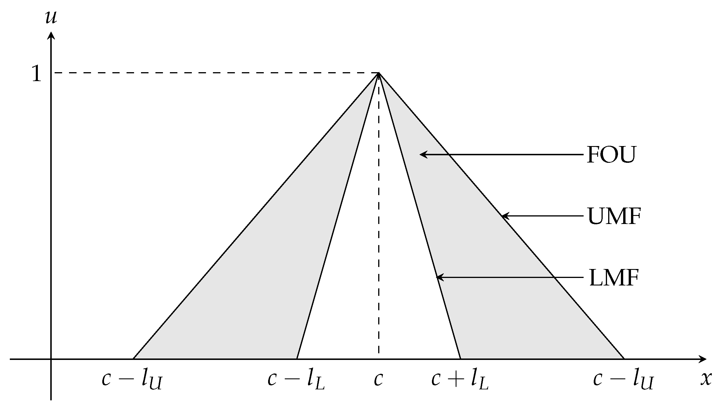
It can be easily seen from Definition 6 that T2-FS is defined on a three-dimensional space. To better characterize its features, Mendel and John [43] defined the information it mapped to the two-dimensional plane as the footprint of uncertainty (FOU).
Definition 7. (Mendel and John [43]) For any , let the primary membership function of a T2-FS S be , then the FOU of S is the union of all the primary membership functions and, thus, can be expressed as
The upper and lower bounds of the FOU are called the upper membership function (UMF) and lower membership function (LMF) of S, respectively.
Definition 8. (Mendel et al. [22]) For a T2-FS S who has an N-element discrete universe of discourse X and primary membership functions , an embedded T1-FS has N elements, one each from , namely , i.e.,
Remark 1.
The embedded T1-FS can be extended to the continuous situations and expressed as
Obviously, there are uncountable numbers of embedded T1-FSs in infinite domains.
Definition 9. (Liu and Liu [11]) Let S be a T2-FV, then the secondary possibility distribution function, , is a map satisfying , and the type-2 possibility distribution function, , is a map satisfying .
Remark 2.
In fact, for a given , in Definition 9 is exactly the secondary MF, , in Definition 6. Therefore, in Definition 9 can also be regarded as the primary MF in Definition 6.
Definition 10. (Men at al. [44]) For any and , if is identically equal to 1, then the T2-FS S is an interval T2-FV (IT2-FV).
According to Definition 10, the secondary membership of an IT2-FV is unique and equal everywhere, i.e., the uncertainty of the MF and the information of the third dimension for an IT2-FV can be ignored, and the IT2-FV can be uniquely determined by the region bounded by its UMF and LMF.
3. Symmetric Triangular Interval Type-2 Fuzzy Variable
In this section, a special kind of IT2-FV, named regular symmetric triangular IT2-FV, is introduced.
3.1. RSTIT2-FV and Its Medium
The specific definition of the IT2-FV studied in this paper is as follows.
Definition 11.
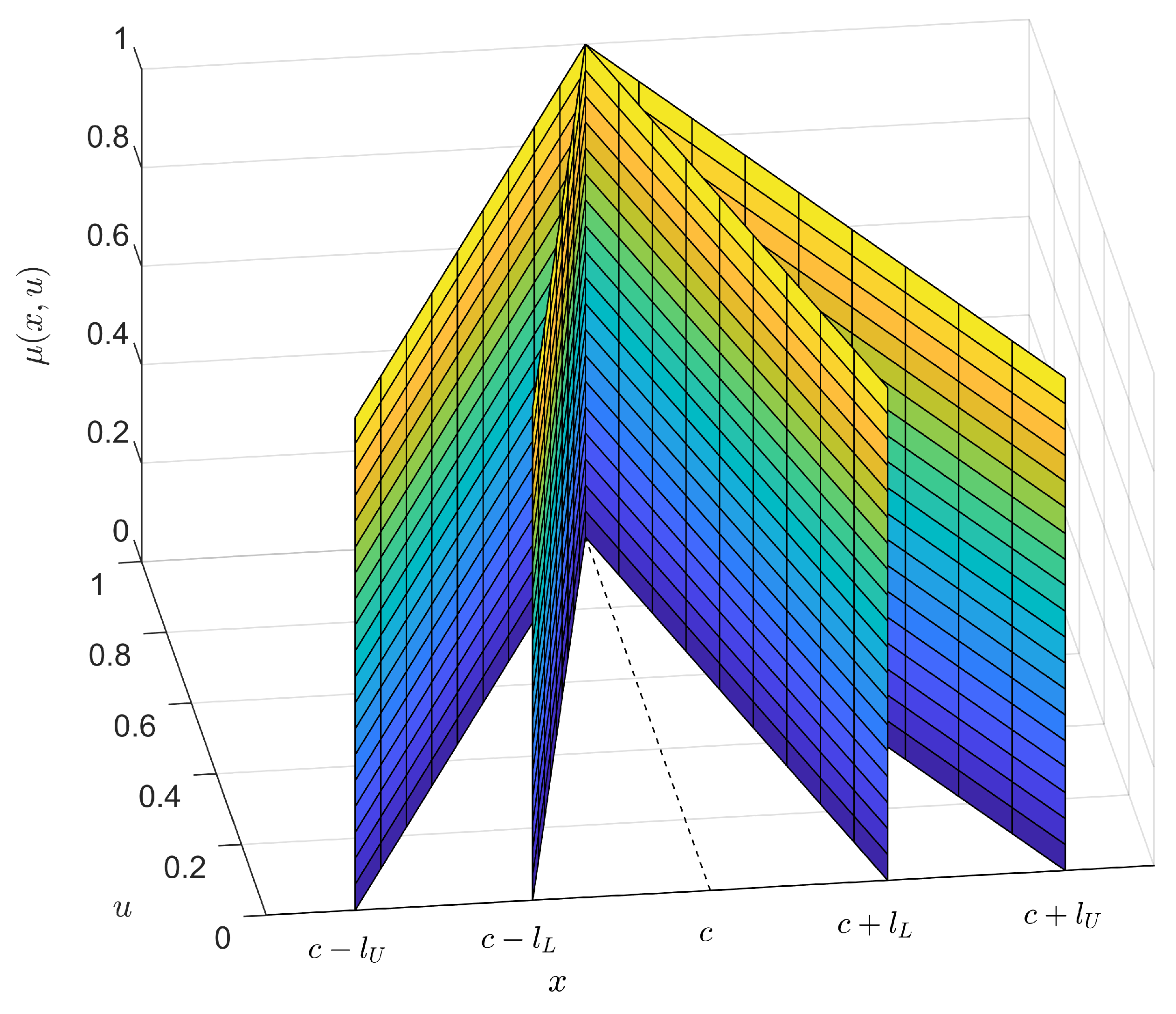
An IT2-FV S is called a regular symmetric triangular IT2-FV (RSTIT2-FV) if its UMF and LMF are as in the following forms,
and
and can be denoted as , where the spreads of the UMF and LMF, and , satisfy , and the peak of them, 1, are reached when x is equal to c.
An RSTIT2-FV is visualized in Figure 1 and Figure 2, respectively, in a three-dimensional space and two-dimensional plane, respectively, and Figure 2 can be understood as a top view of Figure 1.
In order to facilitate the subsequent definitions of credibility distribution and operational law for the RSTIT2-FV, the medium of an RSTIT2-FV is defined in advance.
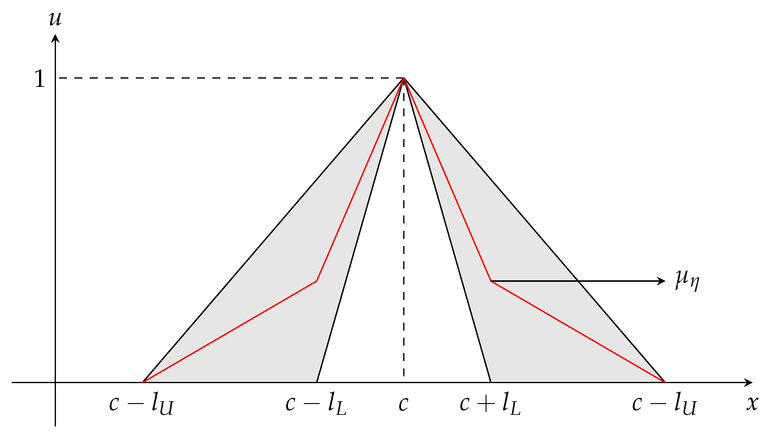
Definition 12.
Let S be an RSTIT2-FV, η be a T1-FV, and their MFs satisfy
then η is called the medium of S.
Definition 12 endows equal weights to every possible value of the MFs for a certain x, it is a relatively evenhanded way to eliminate the uncertainty of MFs in an uncertain and complex environment. Following from Definition 12, the analytical expression of can be calculated as
according to Equations (1) and (2). Figure 3 shows the medium with the red polyline representing its MF, from which we can readily infer that is a regular LR-FV. Moreover, can be regarded as one of the embedded type-1 sets of S, according to Definition 8.
3.2. The Credibility Distribution of the RSTIT2-FVs
By means of the medium , we can define the credibility distribution and inverse credibility distribution in light of Liu [41]’s definition of credibility measure for the T1-FVs. Beforehand, the definition of the credibility measure for an RSTIT2-FV is given.
Definition 13.
Let S be an RSTIT2-FV with the medium of η, and A be a fuzzy event from the universe, then the possibility, necessity, and credibility measures of A for S are, respectively,
It can be easily proven that the credibility measure of an RSTIT2-FV is self-dual and satisfies the monotonicity.
Theorem 1.
For a fuzzy event A from the universe and the credibility measure of an RSTIT2-FV, , we have
Proof.
According to Definition 13, it can be deduced that
□
Theorem 2.
Suppose that C and D are two fuzzy events satisfying , then for the credibility measure of the RSTIT2-FV, we have .
Proof.
In light of Definition 13, it can be obtained that
On the other hand, we have since C is a subset of D. Thus, we can further obtain
Again, on the basis of Definition 13, we have
Based on Definition 13 and Theorems 1 and measure-mono, the possibility, necessity, and credibility measures of a specific fuzzy event for an RSTIT2-FV S can be calculated by
Next, we can define the credibility distribution of S as follows.
Definition 14.
Suppose that S is an RSTIT2-FV with a medium of η, then the credibility distribution of S is defined as .
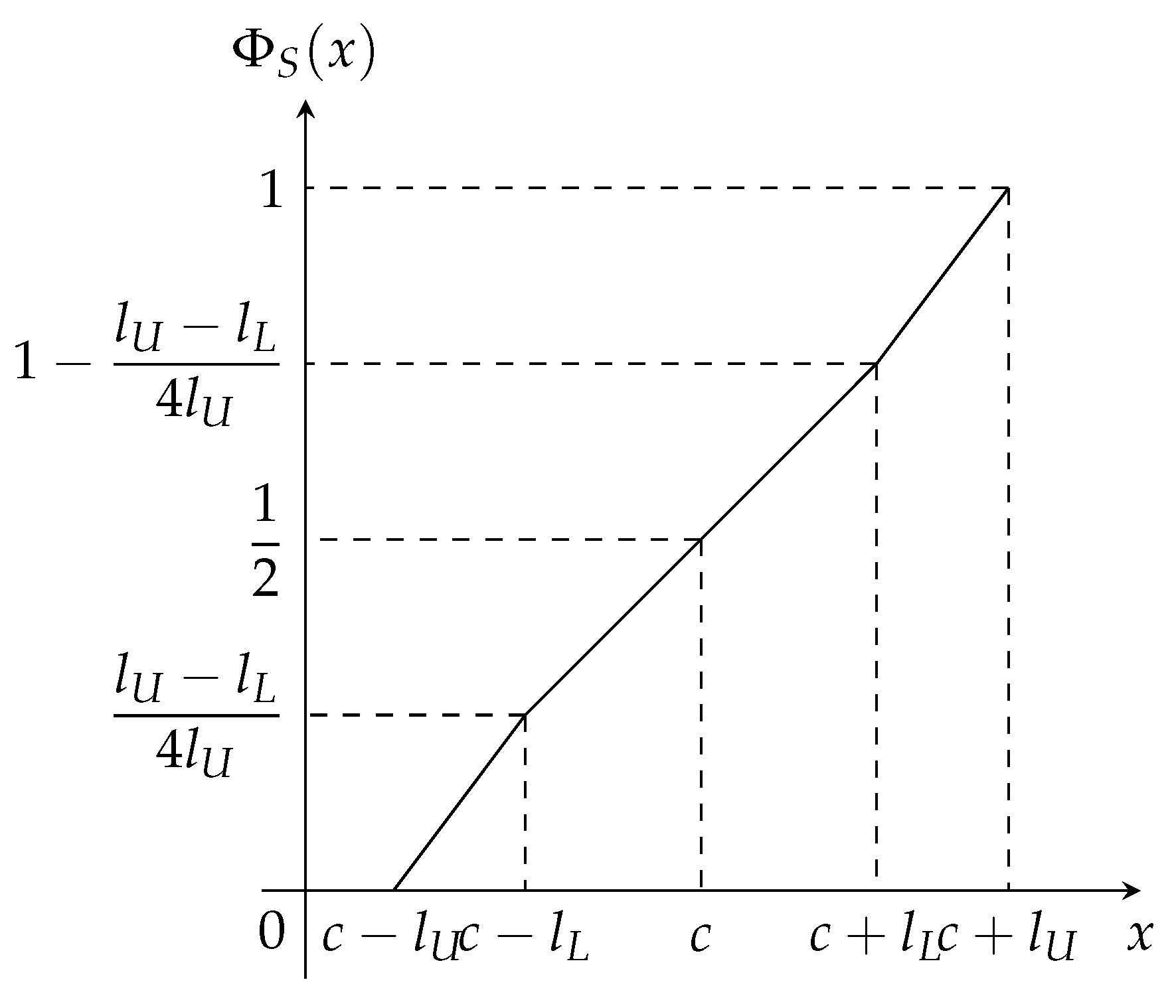
Then by using Definition 14 and Equations (1) and (6), the credibility distribution can be easily calculated as
Figure 4 gives the visualization of . Obviously, is a continuous and strictly increasing function.
Definition 15.
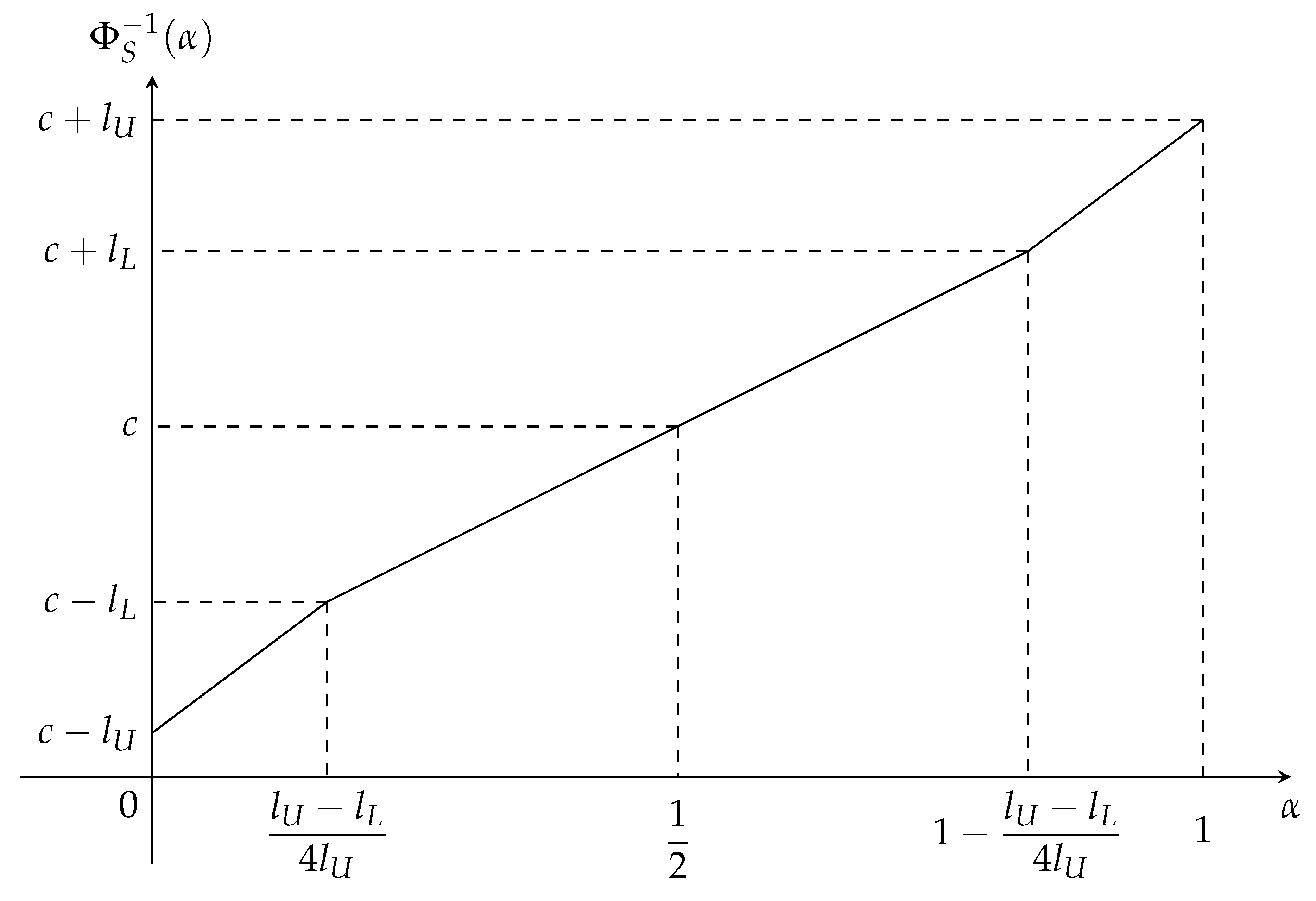
Let S be an RSTIT2-FV, then its inverse credibility distribution is defined as the inverse function of (see Figure 5) and can be calculated by
Remark 3.
Example 1.
Denote an RSTIT2-FV as , then according to Definition 11, we have and , and the UMF and LMF are, respectively,
Afterwards, based on Equation (3) in Definition 12, the MF of the medium for is
Consequently, on the basis of Definition 14, the possibility of the fuzzy event is
and the necessity of it is
Thus, following from Definition 13 and Equation (14), the credibility (credibility distribution) is
Finally, with a view to Equation (9) in Definition 15, we have
Example 2.
In the previous subsection, the credibility distribution and the inverse credibility distribution for a single RSTIT2-FV had been given. Now, we consider a situation where more than one RSTIT2-FV are involved in an arithmetic operation.
Definition 16.
Assume that are RSTIT2-FVs with the mediums of , , respectively, and f is a function from to , then the credibility distribution of , is defined as
where is the medium of S. The inverse credibility distribution of S is the inverse function of , i.e., .
Remark 4.
According to Definition 16, it can be easily deduced that .
4. Operational Law
This section introduces the operational law for fuzzy arithmetic operations regarding RSTIT2-FVs, which can help efficiently calculate in Definition 16. As a prerequisite for its application, the definition of independence is introduced at first.
4.1. Independence
Although Liu and Liu [11] has given the definition of independence for T2-FVs based on the possibility measure, it is somewhat more complex and is not that practicable. Therefore, a new definition of independence based on the credibility measure and the concept of medium in Definition 13 is proposed in this section.
Definition 17.
The RSTIT2-FVs . are said to be mutually independent if
for any subsets .
Definition 18. (Liu and Gao [46]) Let be n T1-FVs, they are said to be mutually independent if
for any subsets .
Remark 5.
Since the independence of the RSTIT2-FVs are derived from their credibility measures, and the credibility measure of the RSTIT2-FVs are based on their mediums, T1-FVs , once RSTIT2-FVs are mutually independent, it means that
holds. Thus, according to Definition 18, the mediums are also mutually independent.
4.2. Operational Law for Strictly Monotone Function of RSTIT2-FVs
Prior to the introduction of the operational law, the definition of the strictly monotone function is set forth.
Definition 19. (Zhou et al. [40]) A real-valued function is said to be strictly monotone if it is strictly increasing with respect to and strictly decreasing with respect to ; that is,
whenever for and for , and
whenever for and for .
Theorem 3.
(Zhou et al. [40]) Let be independent regular LR FVs with the credibility distributions of , respectively. If the function is strictly increasing with respect to and strictly decreasing with respect to , then the inverse credibility distribution of
can be calculated by
Theorem 4.
Suppose that are mutually independent RSTIT2-FVs with the mediums of , respectively. If the function is strictly increasing with respect to and strictly decreasing with respect to , then
has the inverse credibility distribution of
Proof.
Since are the mediums of the RSTIT2-FVs , according to Definition 16, we have
Let , then Definition 16, we have
By using Theorem 3, it can be deduced that
Accordingly, we can easily obtain that
□
In order to show the efficiency of our proposed operational law in calculating the inverse credibility distribution of the fuzzy arithmetic operations, we present three comparative examples, as follows.
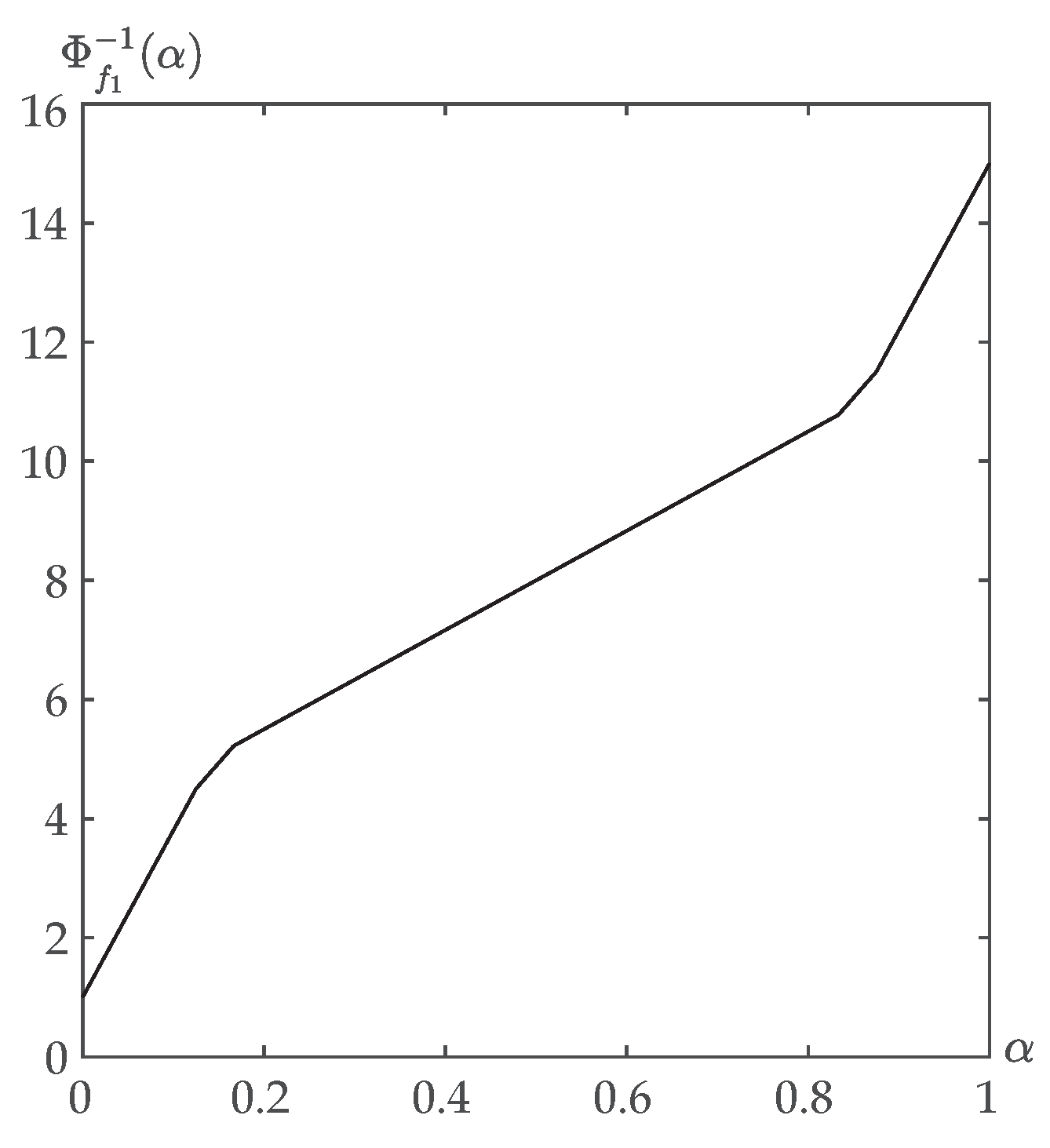
Example 3.
Suppose that in Example 1 and in Example 2 are mutually independent RSTIT2-FVs, and are three functions of them. Then the inverse credibility distributions of can be given directly by Equation (12).
Case 1: Set . It is obviously seen that is strictly increasing with respect to and . Hence, on the basis of Theorem 4 and Equations (10) and (11), we have
Figure 6 provides the graph of .
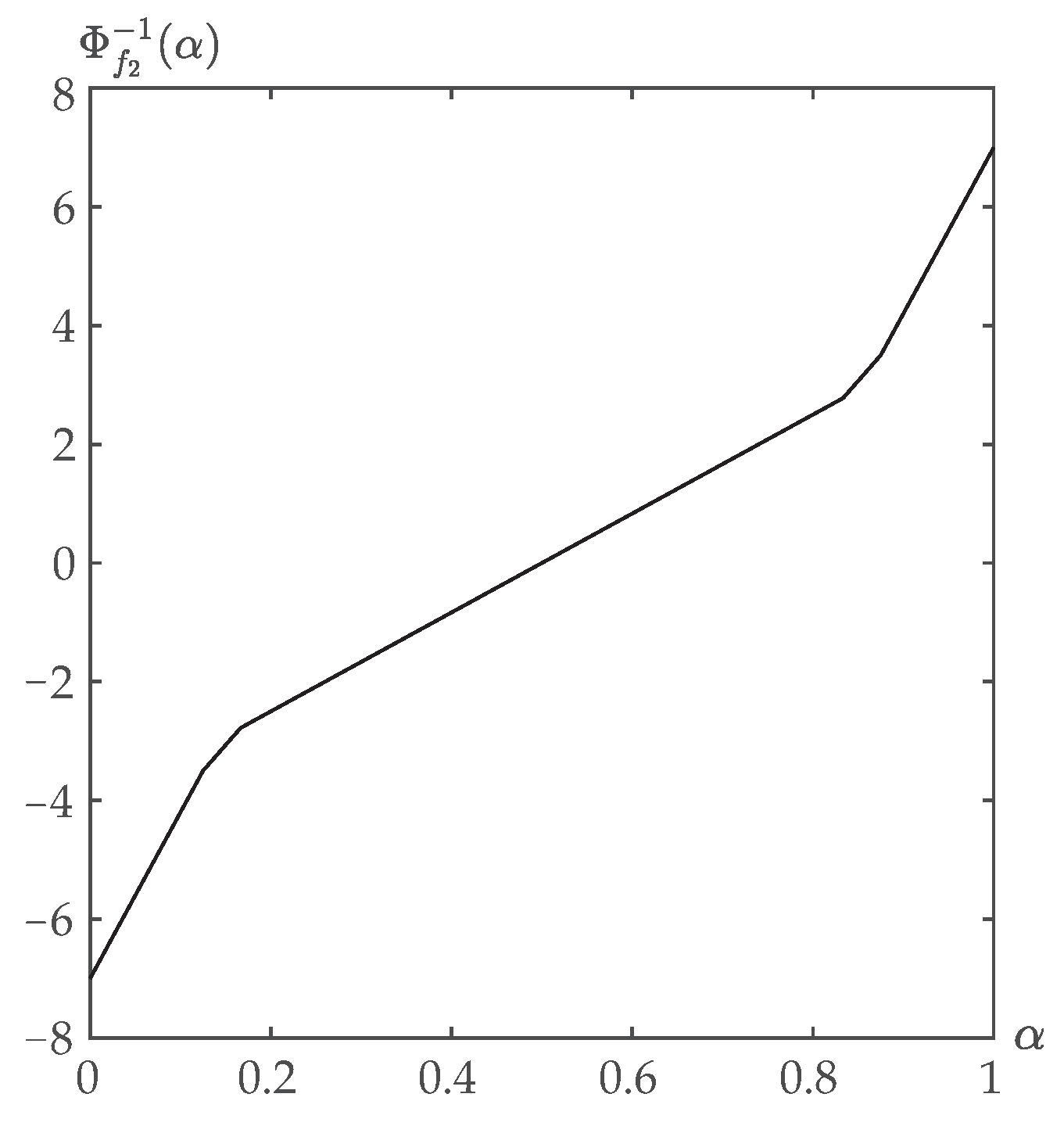
Case 2: Set . In this case, is strictly increasing with respect to , and strictly decreasingm with respect to . Following from Equation (11), we have
Then, with a view to Theorem 4 and Equations (10) and (14), we can readily obtain that
which can be visualized in Figure 7.
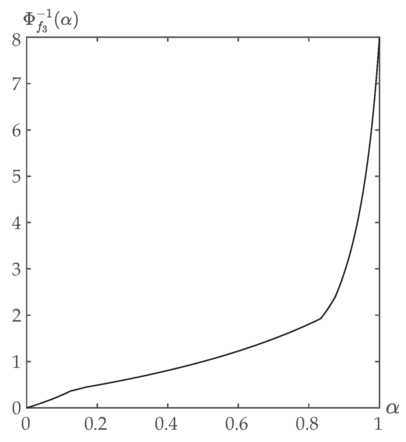
Case 3: Set . Similarly, is strictly increasing with respect to , and strictly decreasing with respect to . According to Equation (10)
Comparatively, if we calculate the inverse credibility function of by means of Zadeh’s extension principle [1], we should first determine the turning points of the MF of the medium for by identifying the key values of and , and then calculate the MF and credibility distribution . Due to space limitations, the solution process is placed in Appendix A, from which we can see that the operational law proposed in this paper can simplify the fuzzy operations without computing the intermediate procedures and possess the correctness.
5. Expected Value
The expected value operator is a crucial numerical characteristic of fuzzy variables; however, to the best of our knowledge, there is not yet a clear expected value definition for the IT2-FVs in the existing literature. Therefore, we define the expected value of the IT2-FVs as well as their strictly monotone functions via the credibility distribution in this section.
Definition 20.
Suppose that S is an RSTIT2-FV or an FV derived from multiple RSTIT2-FVs operations, then the expected value of S can be defined as
Obviously, both integrals in Equation (18) are finite.
Theorem 5.
Given that S is an RSTIT2-FV or obtained from multiple RSTIT2-FVs operations, then its expected value can be simplified as the following form
Proof.
In light of Definitions 5 and 20, we have
□
Example 4.
By means of Theorem 5, the expected value of the RSTIT2-FV in Example 1 is
Analogously, the excepted value of in Example 2 can be calculated as
From Example 4, it can be observed that . In fact, we can easily obtain that the expected value of an RSTIT2-FV S determined by the MF is constantly equal to the center value c, i.e.,
where is the inverse credibility distribution of S, which can be calculated by Equation (9). The results show that the expected value operator we defined is an unbiased estimation.
Example 5.
Following from Theorem 5 and Equation (13), the expected values of in Example 3 can be calculated as
In a similar way, we can get and .
Theorem 6.
Let S be an RSTIT2-FV and k be a constant, then we have
Proof.
When , it is easy to know from Definition 4 that the inverse credibility distribution of is . Then, by using Theorem 5, it can be deduced that
when , the inverse credibility distribution of is , then we have
□
Theorem 7.
Let and be two mutually independent RSTIT2-FVs, then the linearity of the expected value operator concerning the two RSTIT2-FVs can be expressed in the following form,
Proof.
When and , is strictly increasing monotone with respect to and and, thus, the inverse credibility distribution of can be easily obtained as in the views of Definition 4. Following that, and based on Theorems 5 and 6, we have
when and , is strictly increasing with respect to but strictly decreasing with respect to . It follows immediately from Theorems 5 and 6 that
In the other two cases (i.e., and , and ), it is easy to verify that Theorem 7 still holds. Due to space limitations, the details of the proofs are not provided in this paper. □
Remark 6.
Definition 7 can be extended to the general case as
where are mutually independent RSTIT2-FVs and are constants.
Theorem 7 and Remark 6 demonstrate that the introduced expected value operator is consistent with the property of linearity, which can help calculate the expected values of the functions of mutually independent RSTIT2-FVs without calculating the inverse credibility distribution of these RSTIT2-FVs.
Example 6.
On the basis of Theorem 7 and Example 4, the expected value of the RSTIT2-FV in Example 3 can be easily calculated by
which is equal to the result figured out by the integral form in Example 5.
6. Conclusions
In this paper, we defined a special kind of TIT2-FV based on the most typical and simplest symmetric triangular type-1 FV, and proposed a novel operational law to calculate the arithmetic operations for the strictly monotone functions of the mutually independent RSTIT2-FVs as well as the expected value operator via the inverse credibility distribution. The comparative results of the numerical examples verified that the operational law is conducive to simplify the calculation processes, and the expected value operator is an unbiased estimator possessing the property of linearity. Thus, it can be applied to many areas involving complex fuzzy operations.
It is noteworthy that the methodology presented in this paper are not confined to the symmetric and triangular types, but could also be extended to the asymmetric cases and many other types of type-2 fuzzy variables, such as trapezoidal and normal TIT2-FVs, and the regularity of the TIT2-FVs can be extended to more generalized cases, which would be analyzed in the near future. In other words, the proposed method is a universal methodology, providing new insight for future research of many scholars, in both theory and practice, regarding the type-2 fuzzy set theory.
Author Contributions
Conceptualization, J.C.; formal analysis, J.C.; investigation, H.L.; methodology, J.C. and H.L.; software, J.C.; supervision, H.L.; validation, H.L., J.C.; writing—original draft, H.L., J.C.; writing—review and editing, H.L. All authors have read and agreed to the published version of the manuscript.
Funding
This research is supported by the National Natural Science Foundation of China (grant no. 71872110).
Institutional Review Board Statement
Not applicable.
Informed Consent Statement
Not applicable.
Acknowledgments
The authors especially thank the editors and anonymous reviewers for their kind reviews and helpful comments. Any remaining errors are ours.
Conflicts of Interest
We declare that we have no relevant or material financial interests that relate to the research described in this paper. The manuscript has neither been published before, nor has it been submitted for consideration of publication in another journal.
Abbreviations
The following abbreviations are used in the manuscript:
| IT2-FV | interval type-2 fuzzy variable |
| RSTIT2-FV | regular symmetric triangular Interval type-2 fuzzy variable |
| T2-FS | type-2 fuzzy set |
| MF | membership function |
| FV | fuzzy variable |
| T2-FV | type-2 fuzzy variable |
| UMF | upper membership function |
| LMF | lower membership function |
| T1-FS | type-1 fuzzy set |
| T1-FV | type-1 fuzzy variable |
| FOU | footprint of uncertainty |
Appendix A
Example A1.
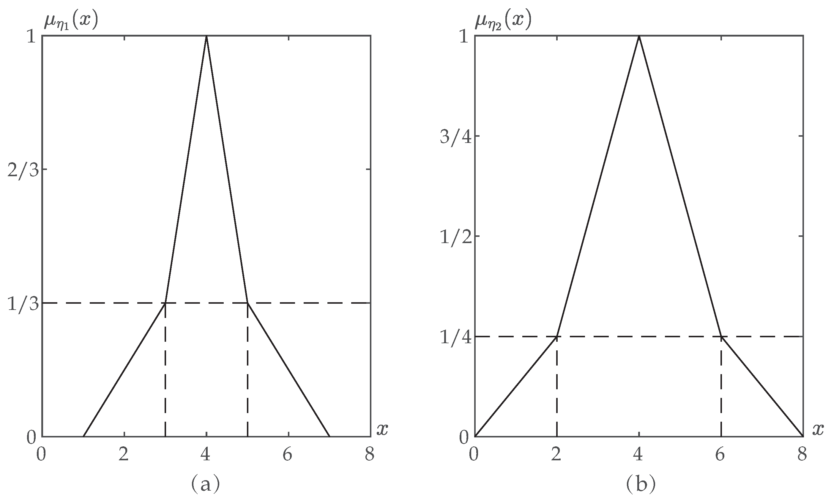
In views of Example 1, the key values of for are, respectively, (1, 0), (3, 1/3), (4, 1), (5, 1/3) and (7, 0), as shown in Figure A1a. Similarly, those of for are, respectively, (0, 0), (2, 1/4), (4, 1), (6, 1/4) and (8, 0), as Figure A1b shows.
According to Zadeh’s extension principle [1], the fuzzy operations of and can only be conducted when the MFs are not piecewise functions. That is, the MFs of the medium for the functions are piecewise functions which have turning points at and 1, respectively. In order to obtain these turning points, the x values for and for should be calculated (see Table A1). Hence, the key values of can be deduced, as summarized in the last row of Table A1.
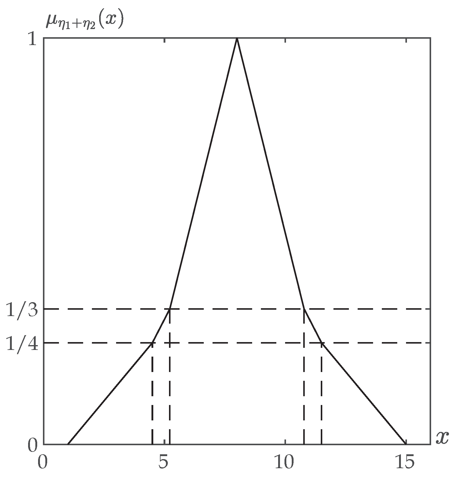
Subsequently, the MF of the medium for is (see Figure A2)
Accordingly, the credibility distribution can be obtained as
and the inverse credibility distribution is
Analogously, on the basis of the x values for and at and 1, the key values of the mediums for can be derived, as shown in Table A2 and Figure A3.
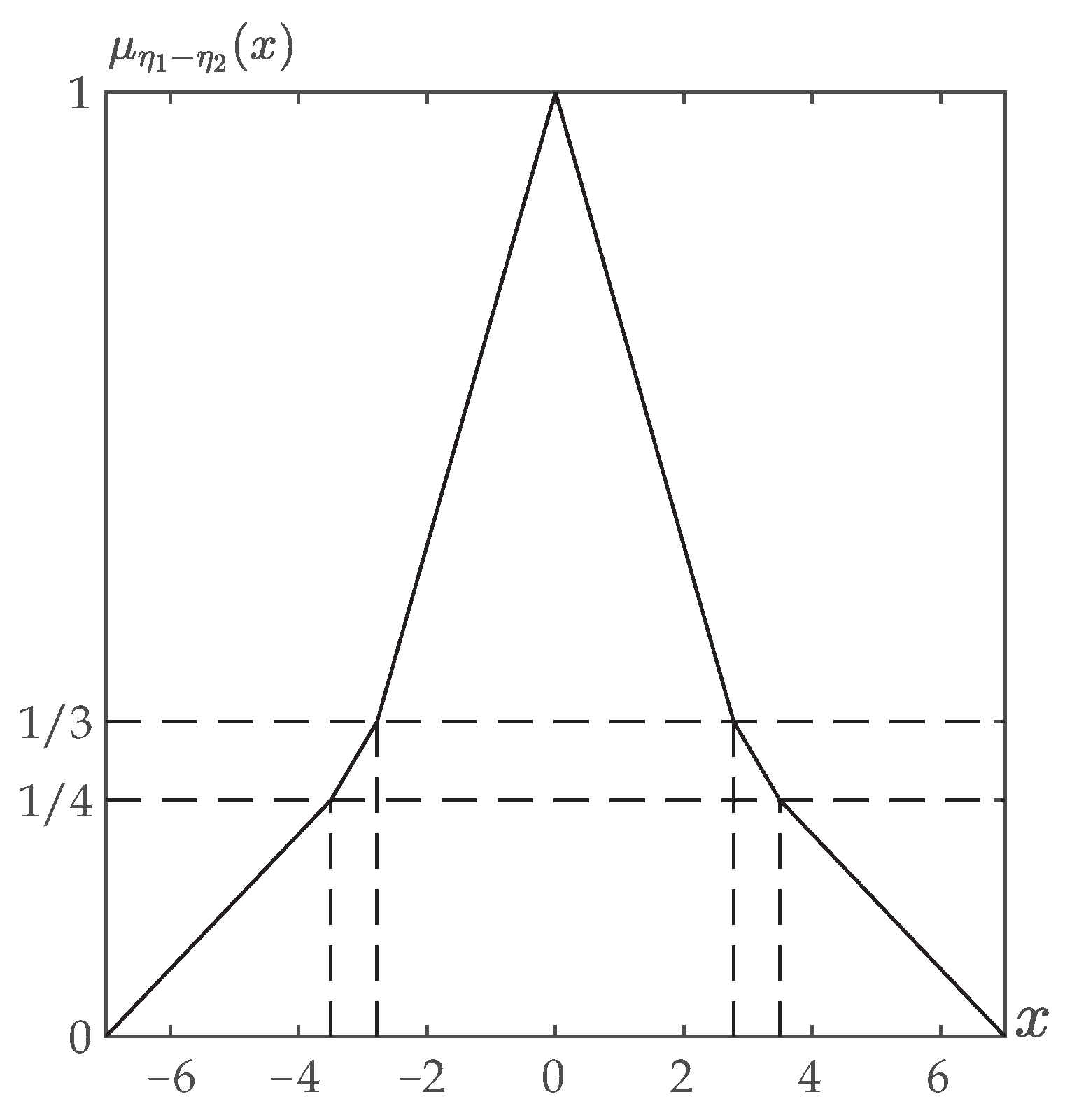
Then, we have the MF of
Then, the credibility distribution is
and the inverse credibility distribution is
which is identical with Equation (15).
Figure A1.
The MF of for (a) and for (b).


Table A1.
The key values of the MFs of the mediums for , and .
| 0 | 1/4 | 1/3 | 1 | 1/3 | 1/4 | 0 | |
|---|---|---|---|---|---|---|---|
| x for | 1 | 5/2 | 3 | 4 | 5 | 11/2 | 7 |
| x for | 0 | 2 | 20/9 | 4 | 52/9 | 6 | 8 |
| x for | 1 | 9/2 | 47/9 | 8 | 97/9 | 23/2 | 15 |
Figure A2.
The MF of .

Table A2.
The key values of the MFs of the mediums for , and .
| 0 | 1/4 | 1/3 | 1 | 1/3 | 1/4 | 0 | |
|---|---|---|---|---|---|---|---|
| x for | 1 | 5/2 | 3 | 4 | 5 | 11/2 | 7 |
| x for | −8 | −6 | −52/9 | −4 | −20/9 | −2 | 0 |
| x for | −7 | −7/2 | −25/9 | 0 | 25/9 | 7/2 | 7 |
Figure A3.
The MF of .

Table A3.
The key values of the MF of the medium for .
| 0 | 1/4 | 1/3 | 1 | 1/3 | 1/4 | 0 | |
|---|---|---|---|---|---|---|---|
| x for | 1/7 | 2/11 | 1/5 | 1/4 | 1/3 | 2/5 | 1 |
| x for | 0 | 2 | 20/9 | 4 | 52/9 | 6 | 8 |
| x for | 0 | 4/11 | 4/9 | 1 | 52/27 | 12/5 | 8 |
References
- Zadeh, L.A. Fuzzy sets. Inf. Control 1965, 8, 338–353. [Google Scholar] [CrossRef] [Green Version]
- Kwakernaak, H. Fuzzy random variables. Part I: Definitions and theorems. Inf. Sci. 1978, 19, 1–15. [Google Scholar] [CrossRef] [Green Version]
- Dubois, D.; Prade, H. Twofold fuzzy sets: An approach to the representation of sets with fuzzy boundaries based on possibility and necessity measures. J. Fuzzy Math. 1983, 3, 53–76. [Google Scholar]
- Liu, B. Toward fuzzy optimization without mathematical ambiguity. Fuzzy Optim. Decis. Mak. 2002, 1, 43–63. [Google Scholar] [CrossRef]
- Petchimuthu, S.; Garg, H.; Kamaci, H.; Atagun, A.O. The mean operators and generalized products of fuzzy soft matrices and their applications in MCGDM. Comput. Appl. Math. 2020, 39, 68. [Google Scholar] [CrossRef]
- Kamaci, H.; Petchimuthu, S.; Akcetin, E. Dynamic aggregation operators and Einstein operations based on interval-valued picture hesitant fuzzy information and their applications in multi-period decision making. Comput. Appl. Math. 2021, 40, 127. [Google Scholar] [CrossRef]
- Zadeh, L.A. The concept of a linguistic variable and its application to approximate reasoning—I. Inf. Sci. 1975, 8, 199–251. [Google Scholar] [CrossRef]
- Kundu, P.; Majumder, S.; Kar, S.; Maiti, M. A method to solve linear programming problem with interval type-2 fuzzy parameters. Fuzzy Optim. Decis. Mak. 2019, 18, 101–130. [Google Scholar] [CrossRef]
- Karnik, N.N.; Mendel, J.M. Centroid of a type-2 fuzzy set. Inform. Sci. 2001, 132, 195–220. [Google Scholar] [CrossRef]
- Coupland, S.; John, R. Geometric interval type-2 fuzzy systems. In Proceedings of the Joint 4th Conference of the European Society for Fuzzy Logic and Technology and the 11th Rencontres Francophones sur la Logique Floue et ses Applications, Barcelona, Spain, 7–9 September 2005; pp. 449–454. [Google Scholar]
- Liu, Z.; Liu, Y. Type-2 fuzzy variables and their arithmetic. Soft Comput. 2010, 14, 729–747. [Google Scholar] [CrossRef]
- Qin, R.; Liu, Y.; Liu, Z. Methods of critical value reduction for type-2 fuzzy variables and their applications. J. Comput. Appl. Math. 2011, 235, 1454–1481. [Google Scholar] [CrossRef]
- Roy, S.K.; Maiti, S.K. Reduction methods of type-2 fuzzy variables and their applications to Stackelberg game. Appl. Intell. 2020, 50, 1398–1415. [Google Scholar] [CrossRef]
- Liang, Q.; Karnik, N.N.; Mendel, J.M. Connection admission control in ATM networks using survey-based type-2 fuzzy logic systems. IEEE Trans. Fuzzy Syst. Man C. 2000, 30, 329–339. [Google Scholar]
- Liu, J.; Li, Y.; Huang, G.; Chen, L. A recourse-based type-2 fuzzy programming method for water pollution control under uncertainty. Symmetry 2017, 9, 265. [Google Scholar] [CrossRef] [Green Version]
- Wu, Y.; Xu, C.; Huang, Y.; Li, X. Green supplier selection of electric vehicle charging based on Choquet integral and type-2 fuzzy uncertainty. Soft Comput. 2020, 24, 3781–3795. [Google Scholar] [CrossRef]
- Karmakar, S.; Seikh, M.R.; Castillo, O. Type-2 intuitionistic fuzzy matrix games based on a new distance measure: Application to biogas-plant implementation problem. Appl. Soft Comput. 2021, 106, 107357. [Google Scholar] [CrossRef]
- Seikh, M.R.; Karmakar, S.; Castillo, O. A novel defuzzification approach of Type-2 fuzzy variable to solving matrix games: An application to plastic ban problem. Iran. J. Fuzzy Syst. 2021, 18, 155–172. [Google Scholar]
- Torshizi, A.D.; Zarandi, M.H.F.; Zakeri, H. On type-reduction of type-2 fuzzy sets: A review. Appl. Soft Comput. 2015, 27, 614–627. [Google Scholar] [CrossRef]
- Mittal, K.; Jain, A.; Vaisla, K.S.; Oscar Castillo, O.; Kacprzyk, J. A comprehensive review on type 2 fuzzy logic applications: Past, present and future. Eng. Appl. Artif. Intel. 2020, 95, 103916. [Google Scholar] [CrossRef]
- Shulla, A.K.; Banshal, S.K.; Seth, T.; Basu, A.; John, R.; Muhuri, P. A bibliometric overview of the field of type-2 fuzzy sets and systems. IEEE Comput. Intell. M. 2020, 15, 89–98. [Google Scholar]
- Mendel, J.M.; John, R.I.; Liu, F. Interval type-2 fuzzy logic systems made simple. IEEE Trans. Fuzzy Syst. 2006, 14, 808–821. [Google Scholar] [CrossRef] [Green Version]
- Celik, E.; Gul, M.; Aydin, N.; Gumus, A.T.; Guneri, A.F. A comprehensive review of multi criteria decision making approaches based on interval type-2 fuzzy sets. Knowl.-Based Syst. 2015, 85, 329–341. [Google Scholar] [CrossRef]
- Javanmard, M.; Nehi, H.M. Rankings and operations for interval type-2 fuzzy numbers: A review and some new methods. J. Appl. Math. Comput. 2019, 59, 597–630. [Google Scholar] [CrossRef]
- Hosseini-Pozveh, M.S.; Safayani, M.; Mirzaei, A. Interval type-2 fuzzy restricted boltzmann machine. IEEE Trans. Fuzzy Syst. 2021, 29, 1133–1142. [Google Scholar] [CrossRef]
- Sang, X.; Zhou, Y.; Yu, X. An uncertain possibility-probability information fusion method under interval type-2 fuzzy environment and its application in stock selection. Inf. Sci. 2019, 504, 546–560. [Google Scholar] [CrossRef]
- Wu, T.; Liu, X. A dynamic interval type-2 fuzzy customer segmentation model and its application in E-commerce. Appl. Soft Comput. 2020, 94, 106366. [Google Scholar] [CrossRef]
- Wu, T.; Liu, X.; Qin, J.; Herrera, F. An interval type-2 fuzzy Kano-prospect-TOPSIS based QFD model: Application to Chinese e-commerce service design. Appl. Soft Comput. 2021, 111, 107665. [Google Scholar] [CrossRef]
- Lee, L.W.; Chen, S.M. A new method for fuzzy multiple attributes group decision-making based on the arithmetic operations of interval type-2 fuzzy sets. In Proceedings of the Seventh International Conference on Machine Learning and Cybernetics, Kunming, China, 12–15 July 2008. [Google Scholar]
- Chen, S.M.; Lee, L.W. Fuzzy multiple attributes group decision-making based on the interval type-2 TOPSIS method. Expert Syst. Appl. 2010, 37, 2790–2798. [Google Scholar] [CrossRef]
- Kiraci, K.; Akan, E. A new type-2 fuzzy set of linguistic variables for the fuzzy analytic hierarchy process. Expert Syst. Appl. 2014, 41, 3297–3305. [Google Scholar]
- Kahraman, C.; Oztaysi, B.; Sari, I.U.; Turanoglu, E. Fuzzy analytic hierarchy process with interval type-2 fuzzy sets. Knowl.-Based Syst. 2014, 59, 48–57. [Google Scholar] [CrossRef]
- Toklu, M.C. Interval type-2 fuzzy TOPSIS method for calibration supplier selection problem: A case study in an automotive company. Arab. J. Geosci. 2014, 59, 11–13. [Google Scholar]
- Hesamian, G. Measuring Similarity and Ordering Based on Interval Type-2 Fuzzy Numbers. IEEE Trans. Fuzzy Syst. 2017, 25, 788–798. [Google Scholar] [CrossRef]
- Chutia, R. Ranking interval type-2 fuzzy number based on a novel value-ambiguity ranking index and its application in risk analysis. Soft Comput. 2021, 25, 8177–8196. [Google Scholar] [CrossRef]
- Kilic, M.; Kaya, I. Investment project evaluation by a decision making methodology based on type-2 fuzzy sets. Appl. Soft Comput. 2015, 25, 8177–8196. [Google Scholar]
- Gong, Y.; Dai, L.; Hu, N. Interval type-2 fuzzy information aggregation based on Einstein operators and its application to decision making. Int. J. Innov. Comput. I. 2016, 12, 2011–2026. [Google Scholar]
- Wang, H.; Ju, Y.; Liu, P.; Ju, D.; Liu, Z. Some trapezoidal interval type-2 fuzzy Heronian mean operators and their application in multiple attribute group decision making. J. Intell. Fuzzy Syst. 2018, 35, 2323–2337. [Google Scholar] [CrossRef]
- Aguero, J.R.; Vargas, A. Calculating functions of interval type-2 fuzzy numbers for fault current analysis. IEEE Trans. Fuzzy Syst. 2007, 15, 31–40. [Google Scholar] [CrossRef]
- Zhou, J.; Yang, F.; Wang, K. Fuzzy arithmetic on LR fuzzy numbers with applications to fuzzy programming. J. Intell. Fuzzy Syst. 2016, 30, 71–87. [Google Scholar] [CrossRef]
- Liu, B. Uncertainty Theory, 2nd ed.; Springer: Berlin/Heidelberg, Germany, 2007. [Google Scholar]
- Dubois, D.; Prade, P. Operations on fuzzy numbers. Int. J. Syst. Sci. 1978, 9, 613–626. [Google Scholar] [CrossRef]
- Mendel, J.M.; John, R.I. Type-2 fuzzy sets made simple. IEEE Trans. Fuzzy Syst. 2002, 10, 117–127. [Google Scholar] [CrossRef]
- Men, J.; Jiang, P.; Xu, H. A chance constrained programming approach for hazMat capacitated vehicle routing problem in Type-2 fuzzy environment. J. Clean. Prod. 2019, 237, 117754. [Google Scholar] [CrossRef]
- Liu, B. Theory and Practice of Uncertain Programming; Springer: Berlin/Heidelberg, Germany, 2002. [Google Scholar]
- Liu, Y.; Gao, J. The independence of fuzzy variables in credibility theory and its applications. Int. J. Uncertain. Fuzz. 2007, 15, 1–20. [Google Scholar] [CrossRef]
Figure 1.
The solid visualization of an RSTIT2-FV.

Figure 2.
The plane visualization of an RSTIT2-FV.

Figure 3.
The visualization of the medium .

Figure 4.
The credibility distribution of S, .

Figure 5.
The inverse credibility distribution of S, .

Figure 6.
The inverse credibility function of .

Figure 7.
The inverse credibility function of .

Figure 8.
The inverse credibility function of .

Publisher’s Note: MDPI stays neutral with regard to jurisdictional claims in published maps and institutional affiliations. |
© 2021 by the authors. Licensee MDPI, Basel, Switzerland. This article is an open access article distributed under the terms and conditions of the Creative Commons Attribution (CC BY) license (https://creativecommons.org/licenses/by/4.0/).
Share and Cite
MDPI and ACS Style
Li, H.; Cai, J. Arithmetic Operations and Expected Values of Regular Interval Type-2 Fuzzy Variables. Symmetry 2021, 13, 2196. https://0-doi-org.brum.beds.ac.uk/10.3390/sym13112196
AMA Style
Li H, Cai J. Arithmetic Operations and Expected Values of Regular Interval Type-2 Fuzzy Variables. Symmetry. 2021; 13(11):2196. https://0-doi-org.brum.beds.ac.uk/10.3390/sym13112196
Chicago/Turabian StyleLi, Hui, and Junyang Cai. 2021. "Arithmetic Operations and Expected Values of Regular Interval Type-2 Fuzzy Variables" Symmetry 13, no. 11: 2196. https://0-doi-org.brum.beds.ac.uk/10.3390/sym13112196
Note that from the first issue of 2016, this journal uses article numbers instead of page numbers. See further details here.