
Various Approaches to the Quantitative Evaluation of Biological and Medical Data Using Mathematical Models

 , , ,
, , ,
Abstract
:1. Introduction
2. Trivial Methods and an Overview of the Known Methods
2.1. Thresholding Methods
2.2. Level-Set Methods
2.3. Graph-Cut Methods
2.4. Neural Network Methods
3. Materials and Methods—Optimized Approaches
3.1. Animal Brain Samples
3.2. Histological Staining
3.3. Microscopy
3.4. Mathematical Approaches
3.4.1. RGB Thresholding Algorithm—The First Method
- The RGB thresholding algorithm:
- The OPTICS clustering algorithm (or the Ankerst-Breunig-Kriegel-Sander algorithm):
| Algorithm 1: OPTICS (DB, eps, MinPts) |
| Input: DB, eps= maximum radius, MinPts- number of points required to form a cluster |
| Output: p to the ordered list |
| Step1: for each point p of DB do |
| p.reachability-distance = UNDEFINED |
| for each unprocessed point p of DB do |
| N = getNeighbors(p, eps) |
| mark p as processed |
| Step2: if core-distance(p, eps, MinPts)!= UNDEFINED then |
| Seeds = empty priority queue |
| update(N, p, Seeds, eps, MinPts) |
| Step3: for each next q in Seeds do |
| N’ = getNeighbors(q, eps) |
| mark q as processed |
| output q to the ordered list |
| Step4: if core-distance(q, eps, MinPts)!= UNDEFINED do |
| update(N’, q, Seeds, eps, MinPts) |
| Algorithm 2: update |
| Input: N—neighbor, p—core points, Seeds-priority queue, eps, MinPts |
| Output: updated seeds |
| Step1: coredist = core-distance (p, eps, MinPts) |
| Step2:for each in |
| if is not processed then |
| new-reach-dist = max(coredist, dist()) |
| Step3:if o.reachability-distance == UNDEFINED then // o is not in Seeds |
| o.reachability-distance = new-reach-dist |
| Seeds.insert(o, new-reach-dist) |
| Step4: else // o in Seeds, check for improvement |
| if new-reach-dist < o.reachability-distance then |
| o.reachability-distance = new-reach-dist |
| Seeds.move-up (o, new-reach-dist) |
- Extracting the pixel percentage:
Otsu Binarization
- Kullback–Leibler adaptive thresholding:
3.4.2. New Filtration Method—Second Method
- Filtration based on histogram (black-white images):
- Filtration based on RGB model (colored images):
3.4.3. Third Method—Using the Image J Program
3.4.4. Fourth Method—The Structural Similarity Index Method (SSIM)
4. Results
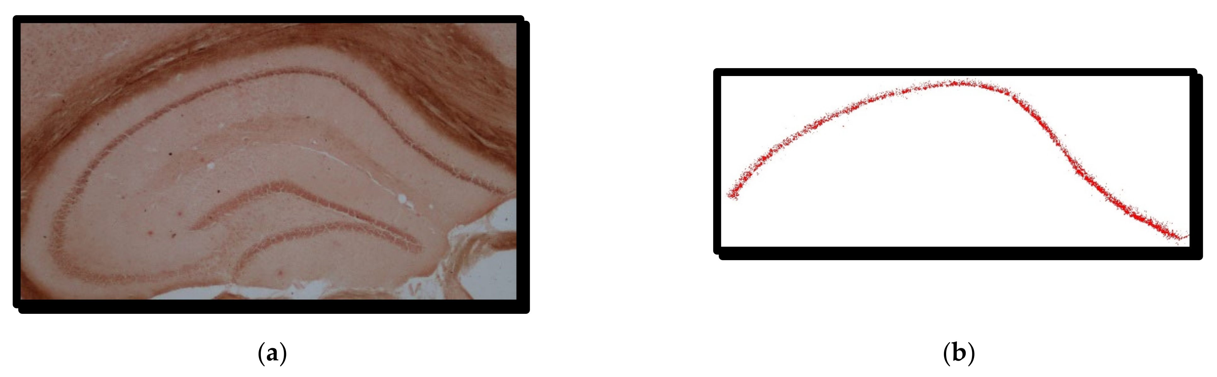
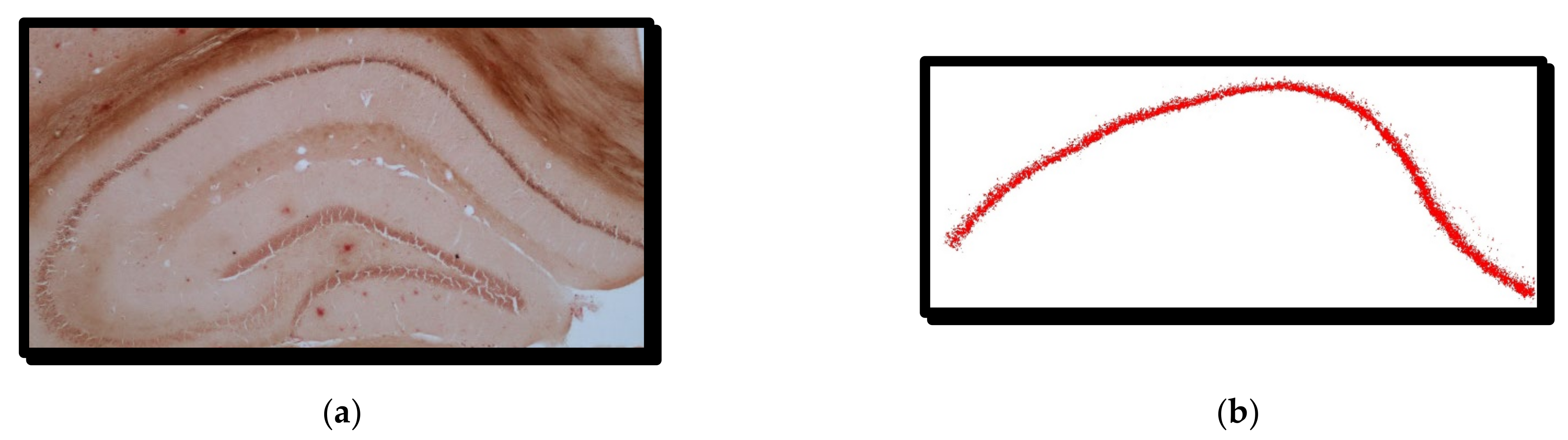
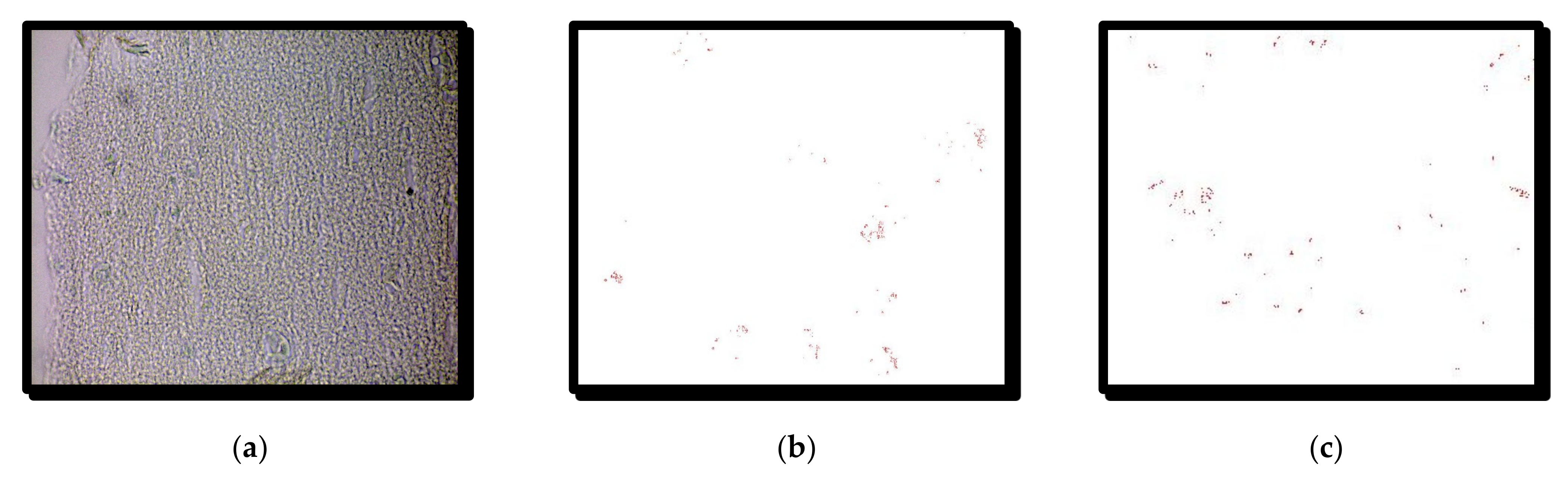
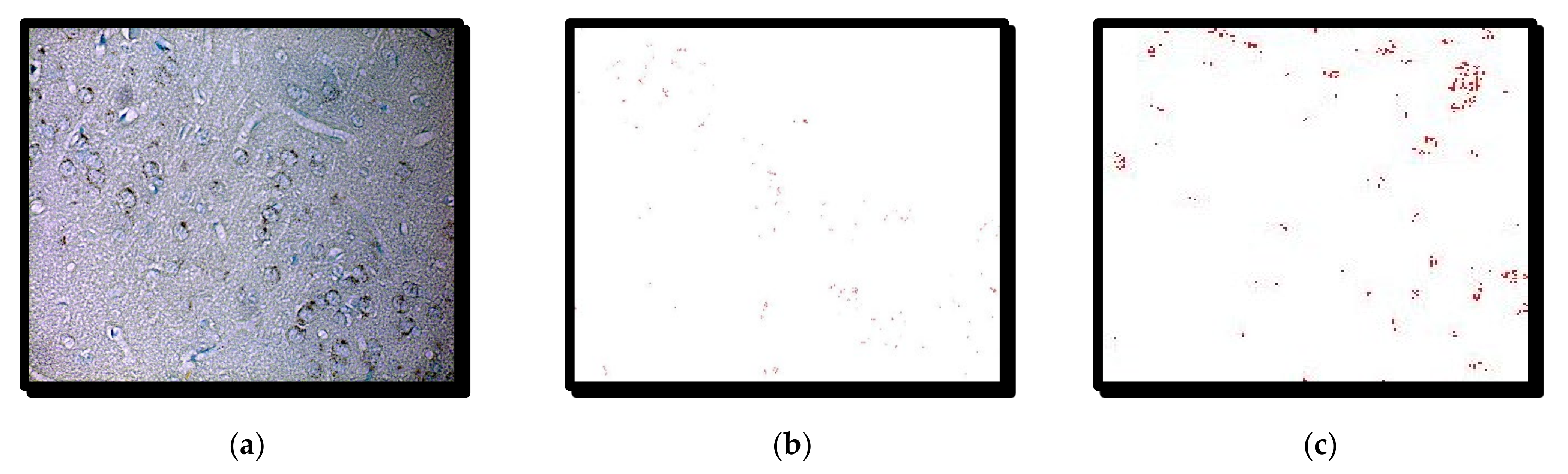
4.1. RGB Thresholding Algorithm—The First Method
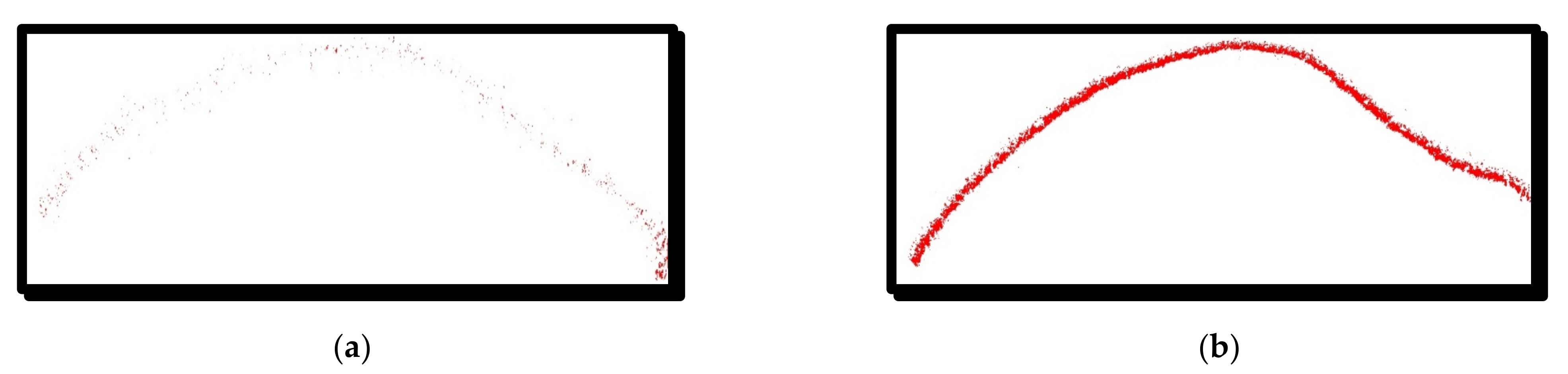
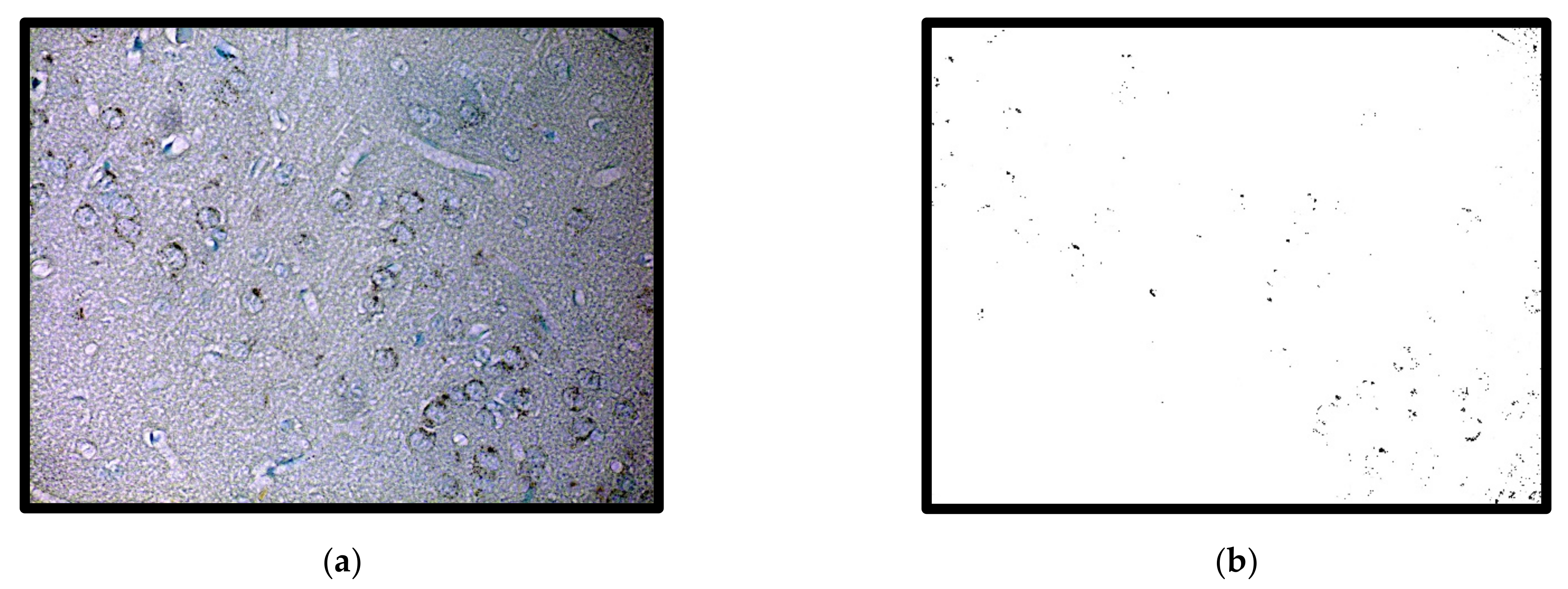
4.2. New Filtration Method—Second Method
4.3. Third Method—Using the Image J Program
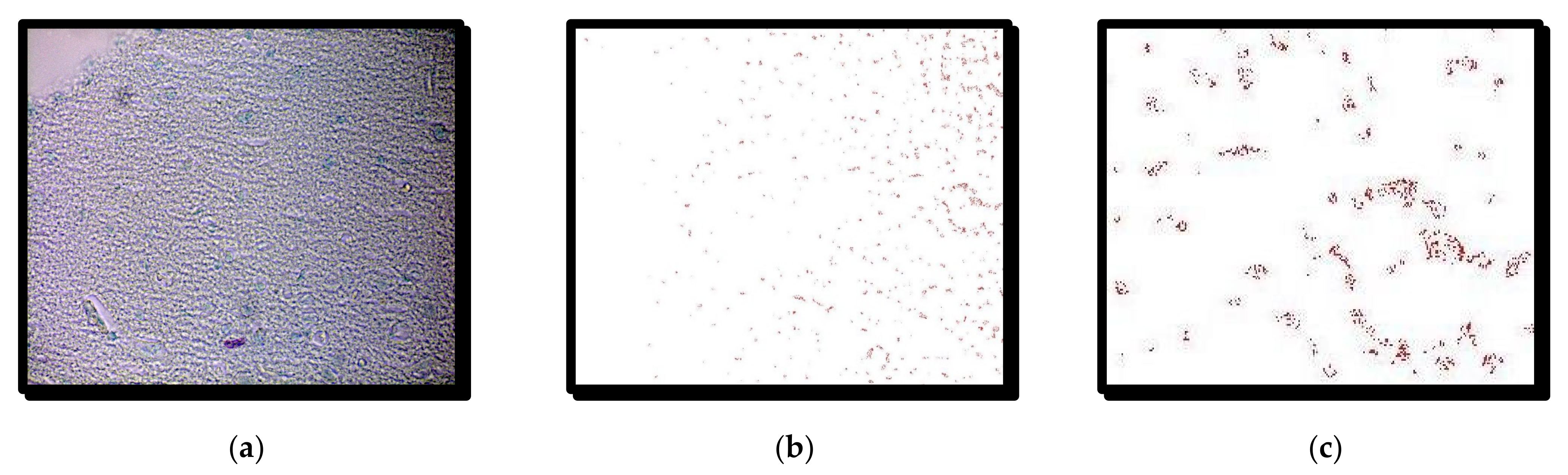
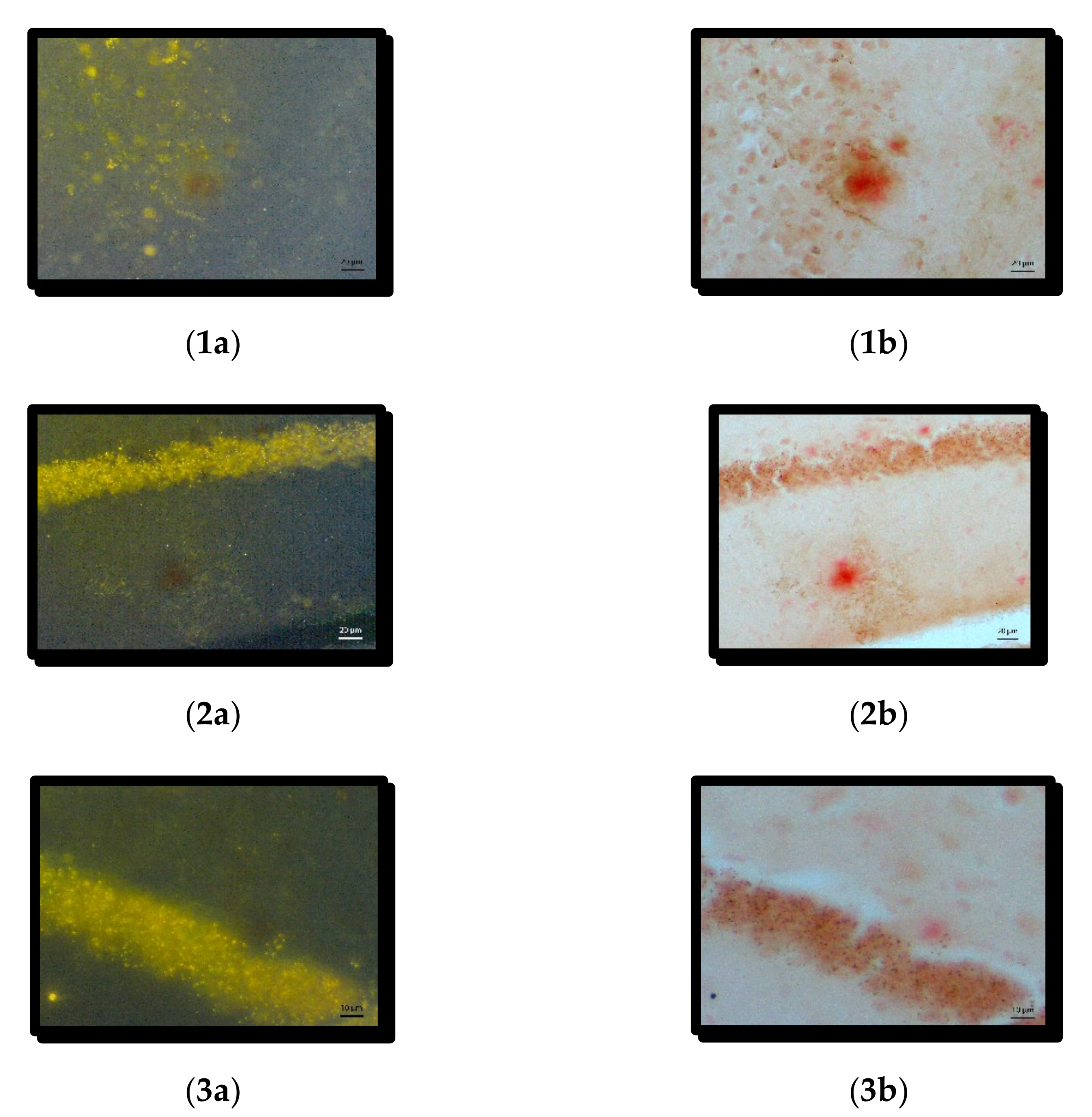
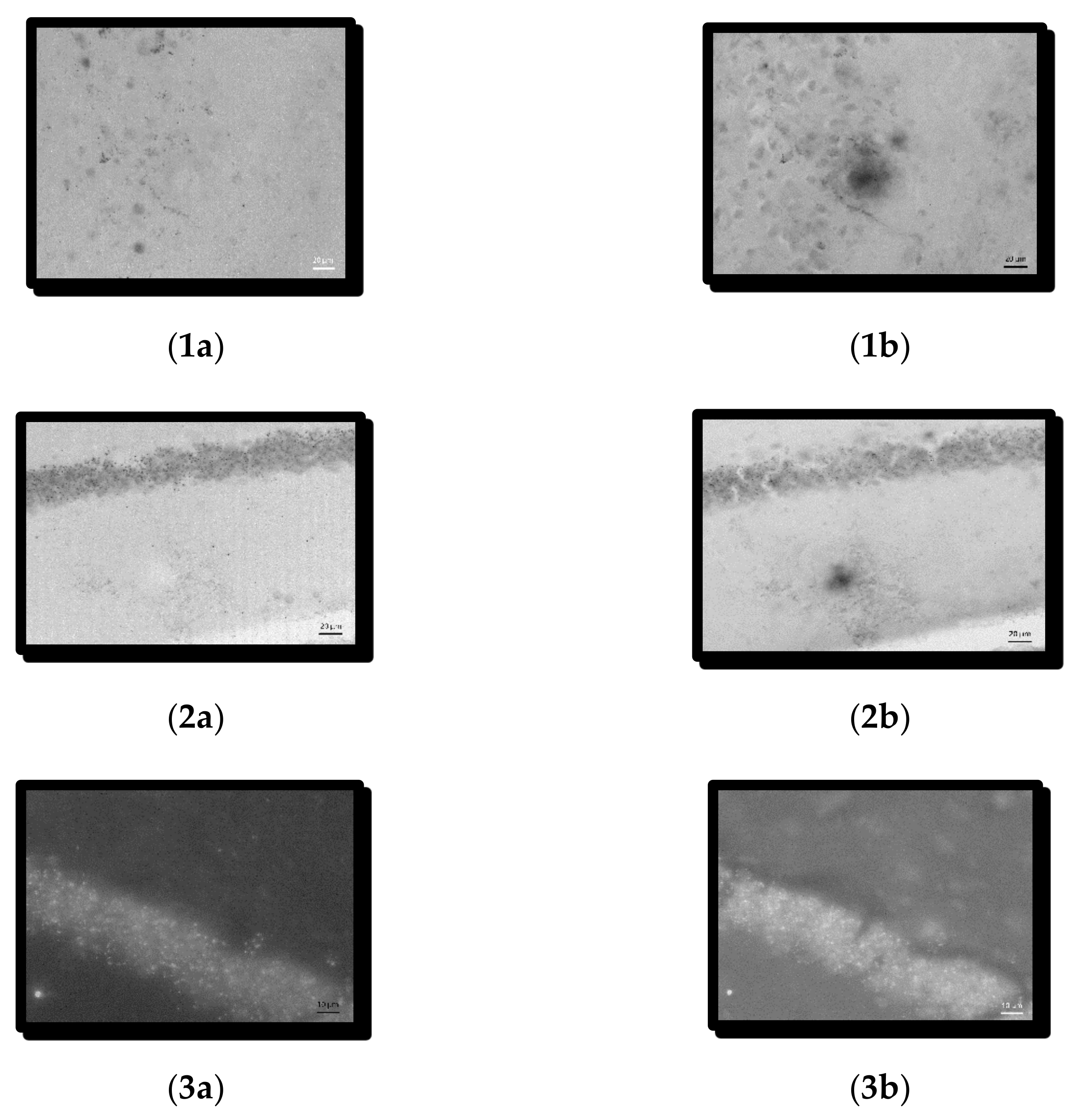
4.4. Symmetry Analysis of Images Photographed in the Bright and Dark Fields of the Light Microscope
5. Discussion
6. Conclusions
Author Contributions
Funding
Institutional Review Board Statement
Informed Consent Statement
Data Availability Statement
Conflicts of Interest
References
- Basavaprasad, B.; Hegadi, R. A Survey on Traditional and Graph Theoretical Techniques for Image Segmentation. Int. J. Comput. Appl. 2014, 975, 8887. [Google Scholar]
- Boykov, Y.Y.; Jolly, M.-P. Interactive Graph Cuts for Optimal Boundary & Region Segmentation of Objects in N-D Images. In Proceedings of the Internation Conference on Computer Vision, Vancouver, BC, Canada, 7–14 July 2001; pp. 105–112. [Google Scholar]
- Boykov, Y.; Veksler, O. Graph Cuts in Vision and Graphics: Theories and Applications BT—Handbook of Mathematical Models in Computer Vision. Handb. Math. Model. Comput. Vis. 2006, 14, 79–96. [Google Scholar]
- Callara, A.L.; Magliaro, C.; Ahluwalia, A.; Vanello, N. A Smart Region-Growing Algorithm for Single-Neuron Segmentation from Confocal and 2-Photon Datasets. Front. Neuroinform. 2020, 14, 9. [Google Scholar] [CrossRef] [Green Version]
- Casadesus, G.; Smith, M.A.; Zhu, X.; Aliev, G.; Cash, A.D.; Honda, K.; Petersen, R.B.; Perry, G. Alzheimer disease: Evidence for a central pathogenic role of iron-mediated reactive oxygen species. J. Alzheimers. Dis. 2004, 6, 165–169. [Google Scholar] [CrossRef] [PubMed]
- Gong, N.; Dibb, R.; Bulk, M.; van der Weerd, L.; Liu, C. Imaging beta amyloid aggregation and iron accumulation in Alzheimer’s disease using quantitative susceptibility mapping MRI. Neuroimage 2019, 191, 176–185. [Google Scholar] [CrossRef]
- Caselli, R.J.; Beach, T.G.; Knopman, D.S.; Graff-Radford, N.R. Alzheimer Disease: Scientific Breakthroughs and Translational Challenges. Mayo Clin. Proc. 2017, 92, 978–994. [Google Scholar] [CrossRef] [Green Version]
- Jankowsky, J.L.; Fadale, D.J.; Anderson, J.; Xu, G.M.; Gonzales, V.; Jenkins, N.A.; Copeland, N.G.; Lee, M.K.; Younkin, L.H.; Wagner, S.L.; et al. Mutant presenilins specifically elevate the levels of the 42 residue β-amyloid peptide in vivo: Evidence for augmentation of a 42-specific γ secretase. Hum. Mol. Genet. 2004, 13, 159–170. [Google Scholar] [CrossRef] [Green Version]
- Peng, B.; Zhang, L.; Zhang, D. A Survey of Graph Theoretical Approaches to Image Segmentation. Pattern Recognit. 2012, 46, 1020–1038. [Google Scholar] [CrossRef] [Green Version]
- Singh, N.; Haldar, S.; Tripathi, A.K.; Horback, K.; Wong, J.; Sharma, D.; Beserra, A.; Suda, S.; Anbalagan, C.; Dev, S.; et al. Brain Iron Homeostasis: From Molecular Mechanisms To Clinical Significance and Therapeutic Opportunities. Antioxid. Redox Signal. 2014, 20, 1324–1363. [Google Scholar] [CrossRef] [PubMed] [Green Version]
- Andersen, H.H.; Johnsen, K.B.; Moos, T. Iron deposits in the chronically inflamed central nervous system and contributes to neurodegeneration. Cell. Mol. Life Sci. 2014, 71, 1607–1622. [Google Scholar] [CrossRef] [Green Version]
- Yang, W.; Cai, L.; Wu, F. Image segmentation based on gray level and local relative entropy two dimensional histogram. PLoS ONE 2020, 15, e0229651. [Google Scholar] [CrossRef]
- Bagga, P.J.; Makhesana, M.A.; Patel, K.; Patel, K.M. Tool wear monitoring in turning using image processing techniques. Mater. Today Proc. 2021, 44, 771–775. [Google Scholar] [CrossRef]
- Zontone, P.; Affanni, A.; Bernardini, R.; Del Linz, L.; Piras, A.; Rinaldo, R. Stress evaluation in simulated autonomous and manual driving through the analysis of skin potential response and electrocardiogram signals. Sensors 2020, 20, 2494. [Google Scholar] [CrossRef] [PubMed]
- Sim, R.; Dias, K.; Martins, R. Dynamic Allocation of SDN Controllers in NFV-based MEC for the Internet of Vehicles. Futur. Internet 2021, 13, 270. [Google Scholar]
- Singh, S.P.; Wang, L.; Gupta, S.; Goli, H.; Padmanabhan, P.; Gulyás, B. 3D Deep Learning on Medical Images: A Review. Sensors 2020, 20, 5097. [Google Scholar] [CrossRef] [PubMed]
- Loucký, J.; Oberhuber, T. Graph cuts in segmentation of a left ventricle from MRI data. In Proceedings of the Czech-Japanese Seminar in Applied Mathematics, Prague and Telč, Czech Republic, 30 August–4 September 2010; pp. 46–54. [Google Scholar]
- Manwar, R.; Zafar, M.; Xu, Q. Signal and Image Processing in Biomedical Photoacoustic Imaging: A Review. Optics 2020, 2, 1. [Google Scholar] [CrossRef]
- Mathur, S.; Shantanu, A.; Rana, A. Estimating the imaging in medical science using image processing techniques. J. Phys. Conf. Ser. 2021, 1714, 012007. [Google Scholar] [CrossRef]
- Zhang, J.; Pang, H.; Cai, W.; Yan, Z. Using image processing technology to create a novel fry counting algorithm. Aquac. Fish 2021. Available online: https://0-www-sciencedirect-com.brum.beds.ac.uk/science/article/pii/S2468550X20301659 (accessed on 23 November 2021).
- Sheikhi, A.; Mehrali, Y.; Tata, M. On the exact joint distribution of a linear combination of order statistics and their concomitants in an exchangeable multivariate normal distribution. Stat. Pap. 2013, 54, 325–332. [Google Scholar] [CrossRef]
- Mesiar, R.; Sheikhi, A. Nonlinear random forest classification, a copula-based approach. Appl. Sci. 2021, 11, 7140. [Google Scholar] [CrossRef]
- He, K.; Zhang, X.; Ren, S.; Sun, J. Deep Residual Learning for Image Recognition. In Proceedings of the 2016 IEEE Conference on Computer Vision and Pattern Recognition (CVPR), Las Vegas, NV, USA, 27–30 June 2016; pp. 770–778. Available online: https://openaccess.thecvf.com/content_cvpr_2016/html/He_Deep_Residual_Learning_CVPR_2016_paper.html (accessed on 23 November 2021).
- Stockman, G.; Shapiro, L.G. Computer Vision, 1st ed.; Prentice Hall PTR: Hoboken, NJ, USA, 2001. [Google Scholar]
- Larbi, M.; Messali, Z.; Hafaifa, A.; Kouzou, A.; Fortaki, T. An image segmentation algorithm based on LSM with stochastic constraint applied to computed tomography images. EEA—Electroteh. Electron. Autom. 2019, 67, 87–96. [Google Scholar]
- Liu, J.; Wei, X.; Li, L.M.R. image segmentation based on level set method. Multimed. Tools Appl. 2020, 79, 11487–11502. [Google Scholar] [CrossRef]
- Jiang, X.; Zhang, R.; Nie, S. Image Segmentation Based on Level Set Method. Phys. Procedia 2012, 33, 840–845. [Google Scholar] [CrossRef] [Green Version]
- Katopodes, N.D. Level Set Method. In Free-Surface Flow; Elsevier: Amsterdam, The Netherlands, 2019; pp. 804–828. [Google Scholar]
- Ždímalová, M.; Major, J.; Kopáni, M. Graph cutting and its application to biological data. Open Phys. 2019, 17, 468–479. [Google Scholar] [CrossRef]
- Yi, F.; Moon, I. Image segmentation: A survey of graph-cut methods. In Proceedings of the 2012 International Conference on Systems and Informatics (ICSAI2012), Yantai, China, 19–20 May 2012; pp. 1936–1941. [Google Scholar] [CrossRef]
- Boykov, Y.; Funka-Lea, G. Graph cuts and efficient N-D image segmentation. Int. J. Comput. Vis. 2006, 70, 109–131. [Google Scholar] [CrossRef] [Green Version]
- Kolmogorov, V.; Zabih, R. What energy functions can be minimized via graph cuts? Lect. Notes Comput. Sci. (Incl. Subser. Lect. Notes Artif. Intell. Lect. Notes Bioinform.) 2002, 2352, 65–81. [Google Scholar] [CrossRef] [Green Version]
- Rueden, C.T.; Schindelin, J.; Hiner, M.C.; DeZonia, B.E.; Walter, A.E.; Arena, E.T.; Eliceiri, K.W. Image J2: Image J for the next generation of scientific image data. BMC Bioinform. 2017, 18, 529. [Google Scholar] [CrossRef]
- Image J. Available online: https://imagej.nih.gov/ij/index.html (accessed on 15 October 2021).
- CellProfiler. Cell Image Analysis Software. Available online: https://cellprofiler.org/ (accessed on 15 October 2021).
- Ilastik the Interactive Learning and Segmentation Toolkit. Available online: https://www.ilastik.org/ (accessed on 15 October 2021).
- Geman, D. Stochastic relaxation, Gibbs distributions and the Bayesian restoration of images. J. Appl. Stat. 1993, 20, 25–62. [Google Scholar] [CrossRef]
- Maeda, J.; Ishikawa, C.; Novianto, S.; Tadehara, N.; Suzuki, Y. Rough and accurate segmentation of natural color images using fuzzy region-growing algorithm. In Proceedings of the 15th International Conference on Pattern Recognition. ICPR-2000, Barcelona, Spain, 3–7 September 2000; IEEE Computer Society: Washington, DC, USA, 2000; Volume 3, pp. 638–641. [Google Scholar]
- Magzhan, K.; Jani, H. A Review and Evaluations of Shortest Path Algorithms. Int. J. Sci. Technol. Res. 2013, 2, 99–104. [Google Scholar]
- Moghaddamzadeh, A.; Bourbakis, N. A fuzzy region growing approach for segmentation of color images. Pattern Recognit. 1997, 30, 867–881. [Google Scholar] [CrossRef]
- Horowitz, S.L.; Pavlidis, T. Picture Segmentation by a Directed Split and Merge Procedure. In Proceedings of the 2nd International Joint Conference on Pattern Recognition, Copenhagen, Denmark, 13–15 August 1974; pp. 424–433. [Google Scholar]
- Ohlander, R.; Price, K.; Reddy, D.R. Picture segmentation using a recursive region splitting method. Comput. Graph. Image Process. 1978, 8, 313–333. [Google Scholar] [CrossRef]
- Jain, S.; Salau, A.O. An image feature selection approach for dimensionality reduction based on kNN and SVM for AkT proteins. Cogent Eng. 2019, 6, 1–14. [Google Scholar] [CrossRef]
- Ždímalová, M.; Krivá, Z.; Bohumel, T. Graph Cuts in Image Processing. In Proceedings of the Aplimat 2015: 14th Conference on Applied Mathematics, Bratislava, Slovak Republic, 3–5 February 2015; Faculty of Mechanical Engineering, Slovak University of Technology: Bratislava, Slovakia, 2015; pp. 774–786. [Google Scholar]
- Watanabe, T.; Tan, Z.; Wang, X.; Martinez-Hernandez, A.; Frahm, J. Magnetic resonance imaging of noradrenergic neurons. Brain Struct. Funct. 2019, 224, 1609–1625. [Google Scholar] [CrossRef] [PubMed] [Green Version]
- Meadowcroft, M.D.; Connor, J.R.; Yang, Q.X. Cortical iron regulation and inflammatory response in Alzheimer’s disease and APPSWE/PS1ΔE9 mice: A histological perspective. Front. Neurosci. 2015, 9, 255. [Google Scholar] [CrossRef] [PubMed] [Green Version]
- Svobodová, H.; Kosnáč, D.; Balázsiová, Z.; Tanila, H.; Miettinen, P.O.; Sierra, A.; Vitovič, P.; Wagner, A.; Polák, S.; Kopáni, M. Elevated age-related cortical iron, ferritin and amyloid plaques in APPswe/PS1ΔE9 transgenic mouse model of Alzheimer’s disease. Physiol. Res. 2019, 68, S445–S451. [Google Scholar] [CrossRef] [PubMed]
- Meguro, R.; Asano, Y.; Odagiri, S.; Li, C.; Iwatsuki, H.; Shoumura, K. Nonheme-iron histochemistry for light and electron microscopy: A historical, theoretical and technical review. Arch. Histol. Cytol. 2007, 70, 1–19. [Google Scholar] [CrossRef] [Green Version]
- Zhang, D.; Islam, M.M.; Lu, G. A review on automatic image annotation techniques. Pattern Recognit. 2012, 45, 346–362. [Google Scholar] [CrossRef]
- Ankerst, M.; Breunig, M.M.; Kriegel, H.; Sander, J. OPTICS: Ordering Points to Identify the Clustering Structure. ACM SIGMOD Rec. 1999, 28, 49–60. [Google Scholar] [CrossRef]
- Breunig, M.M.; Kriegel, H.P.; Ng, R.T.; Sander, J. OPTICS-OF: Identifying local outliers. Lect. Notes Comput. Sci. (Incl. Subser. Lect. Notes Artif. Intell. Lect. Notes Bioinform.) 1999, 1704, 262–270. [Google Scholar] [CrossRef] [Green Version]
- Kriegel, H.; Kröger, P.; Sander, J.; Zimek, A. Density-based clustering. WIREs Data Min. Knowl. Discov. 2011, 1, 231–240. [Google Scholar] [CrossRef]
- Ester, M.; Kriegel, H.P.; Sander, J.; Xiaowei, X. A density-based algorithm for discovering clusters in large spatial databases with noise. In Proceedings of the Second International Conference on Knowledge Discovery and Data Mining (KDD-96), Portland, OR, USA, 2–4 August 1996; AAAI Press: Palo Alto, CA, USA, 1996; pp. 226–231. ISBN 1-57735-004-9. [Google Scholar]
- Otsu, N. A Threshold Selection Method from Gray-Level Histograms. IEEE Trans. Syst. Man. Cybern. 1979, 9, 62–66. [Google Scholar] [CrossRef] [Green Version]
- Kullback, S.; Leibler, R.A. On Information and Sufficiency. Ann. Math. Stat. 1951, 22, 79–86. [Google Scholar] [CrossRef]
- Goh, T.Y.; Basah, S.N.; Yazid, H.; Aziz Safar, M.J.; Ahmad Saad, F.S. Performance analysis of image thresholding: Otsu technique. Measurement 2018, 114, 298–307. [Google Scholar] [CrossRef]
- Lapuyade-Lahorgue, J.; Xue, J.-H.; Ruan, S. Segmenting Multi-Source Images Using Hidden Markov Fields With Copula-Based Multivariate Statistical Distributions. IEEE Trans. Image Process. 2017, 26, 3187–3195. [Google Scholar] [CrossRef] [PubMed] [Green Version]


| Animal | Length of Image (Pixels) | Width of Image (Pixels) | Total Area (Pixels) | Total Iron (Pixels) | Total Iron (%) |
|---|---|---|---|---|---|
| 6 months | 5102 | 1961 | 10,005,022 | 394,419 | 0.039 |
| 8 months | 4776 | 2281 | 10,894,056 | 529,147 | 0.049 |
| 13 months | 5352 | 2497 | 13,363,944 | 701,661 | 0.053 |
| Animal | Length of Image (Pixels) | Width of Image (Pixels) | Total Area (Pixels) | Total Iron (Pixels) | Total Iron (%) |
|---|---|---|---|---|---|
| 6 months | 6889 | 4495 | 30,966,055 | 673,311 | 0.021 |
| 8 months | 6786 | 4271 | 28,983,006 | 727,235 | 0.025 |
| 13 months | 7305 | 3431 | 25,063,455 | 906,655 | 0.036 |
| Animal | Length of Image (Pixels) | Width of Image (Pixels) | Total Area (Pixels) | Total Iron (Pixels) | Total Iron (%) |
|---|---|---|---|---|---|
| 6 months | 5880 | 4593 | 27,006,840 | 698,866 | 0.025 |
| 8 months | 6001 | 3281 | 19,689,281 | 579,981 | 0.029 |
| 13 months | 4800 | 2597 | 12,465,600 | 517,863 | 0.041 |
| Animal | Detected Area (Pixel) | False Positive Area | Net Detected Area | Total Image Area (Pixel) | % |
|---|---|---|---|---|---|
| 10 months old animal | 14,983 | 0 | 14,983 | 4,958,816 | 0.3 |
| 2nd animal | 1653 | 100 | 1553 | 4,958,816 | 0.11 |
| 3rd animal | 6262 | 170 | 6092 | 4,958,816 | 0.12 |
| Animal | Total Area | % |
|---|---|---|
| 10-month-old animal | 15,186 | 0.3 |
| 2nd animal | 11,786 | 0.24 |
| 3rd animal | 13,105 | 0.26 |
| Image Set | SSIM |
|---|---|
| 1a–1b | 0.6512 |
| 2a–2b | 0.7708 |
| 3a–3b | 0.7436 |
Publisher’s Note: MDPI stays neutral with regard to jurisdictional claims in published maps and institutional affiliations. |
© 2021 by the authors. Licensee MDPI, Basel, Switzerland. This article is an open access article distributed under the terms and conditions of the Creative Commons Attribution (CC BY) license (https://creativecommons.org/licenses/by/4.0/).
Share and Cite
Ždímalová, M.; Chatterjee, A.; Kosnáčová, H.; Ghosh, M.; Obaidullah, S.M.; Kopáni, M.; Kosnáč, D. Various Approaches to the Quantitative Evaluation of Biological and Medical Data Using Mathematical Models. Symmetry 2022, 14, 7. https://0-doi-org.brum.beds.ac.uk/10.3390/sym14010007
Ždímalová M, Chatterjee A, Kosnáčová H, Ghosh M, Obaidullah SM, Kopáni M, Kosnáč D. Various Approaches to the Quantitative Evaluation of Biological and Medical Data Using Mathematical Models. Symmetry. 2022; 14(1):7. https://0-doi-org.brum.beds.ac.uk/10.3390/sym14010007
Chicago/Turabian StyleŽdímalová, Mária, Anuprava Chatterjee, Helena Kosnáčová, Mridul Ghosh, Sk Md Obaidullah, Martin Kopáni, and Daniel Kosnáč. 2022. "Various Approaches to the Quantitative Evaluation of Biological and Medical Data Using Mathematical Models" Symmetry 14, no. 1: 7. https://0-doi-org.brum.beds.ac.uk/10.3390/sym14010007