Copula-Based Estimation Methods for a Common Mean Vector for Bivariate Meta-Analyses

Abstract

Traditional bivariate meta-analyses adopt the bivariate normal model. As the bivariate normal distribution produces symmetric dependence, it is not flexible enough to describe the true dependence structure of real meta-analyses. As an alternative to the bivariate normal model, recent papers have adopted “copula” models for bivariate meta-analyses. Copulas consist of both symmetric copulas (e.g., the normal copula) and asymmetric copulas (e.g., the Clayton copula). While copula models are promising, there are only a few studies on copula-based bivariate meta-analysis. Therefore, the goal of this article is to fully develop the methodologies and theories of the copula-based bivariate meta-analysis, specifically for estimating the common mean vector. This work is regarded as a generalization of our previous methodological/theoretical studies under the FGM copula to a broad class of copulas. In addition, we develop a new R package, “CommonMean.Copula”, to implement the proposed methods. Simulations are performed to check the proposed methods. Two real dataset are analyzed for illustration, demonstrating the insufficiency of the bivariate normal model.

1. Introduction

Bivariate outcomes often arise in meta-analyses on scientific studies, such as education and medicine. Educational researchers may analyze bivariate exam scores on verbal and mathematics [1,2], or on mathematics and statistics [3]. Medical experts may analyze bivariate risk scores on myocardial infection and cardiovascular death for diabetes patients [4,5]. Bivariate meta-analyses are statistical methods designed for these meta-analytical studies [6]. Dependence between two outcomes should be considered while performing bivariate meta-analyses. If one simply considers univariate (marginal) analysis for each outcome separately, any possible dependence between the outcomes is ignored. Riley [2] and Copas et al. [7] showed that ignoring the dependence between two outcomes increases the error for estimating parameters due to the loss of information. In medical research, dependence itself can be of clinical importance, e.g., dependence between two survival outcomes in meta-analysis [8,9,10,11].

In the traditional bivariate meta-analyses, the parameters of interest are the means of a bivariate normal model [6]. However, the bivariate normal model is not flexible enough to describe the true dependence structure of real meta-analyses. It will be shown that the bivariate normal mode fits poorly to the dependence structure of real bivariate meta-analyses (Section 8). This has motivated researchers to consider alternative models.

As an alternative to the bivariate normal model, recent papers have adopted “copula” models for bivariate meta-analyses [3,5,12,13,14,15]. Copula models are flexible as they allow a variety of dependence structures. Copulas consist of both symmetric copulas (e.g., the normal copula) and asymmetric copulas (e.g., the Clayton copula). Copula models have become very popular in all areas of science by replacing the traditional multivariate normal models. In astronomy, Takeuchi [16] constructed the bivariate luminosity density functions using the FGM copula; see reference [17] for the application of the FGM copula to engineering. In ecology, Ghosh et al. [18] applied copulas to model the dependence structure in environmental and biological variables. In environmental science, Alidoost et al. [19] used bivariate copulas in the analysis of temperature. See the survey of [20] for applications to energy, forestry, and environmental sciences. The books of [21,22] are devoted to the applications of copulas in survival analysis; see also references [11,23,24,25].

While bivariate copula models for meta-analyses are promising, there are only a few methodologically and theoretically solid studies on copula-based bivariate meta-analysis. For instance, the detailed theoretical studies of [3] are limited to the FGM copula. Other copula-based meta-analyses published in biostatistical journals, such as [5,12,13,14,15], are proposed without theoretical details. Furthermore, copula-based bivariate meta-analyses have not been implemented in a free software environment.

Therefore, the goal of this article is to fully develop the methodologies and theories of the copula-based bivariate meta-analysis for estimating the common mean vector. This work is regarded as a large generalization of our previous methodological/theoretical studies under the FGM copula model [3] to a broad class of copula models. In this article, we obtain theoretical results, including the formula of the information matrix and large sample theories. Our theoretical results guarantee the applications of many copulas, such as the Clayton, Gumbel, Frank, and normal copulas, in addition to the FGM copula. In addition, we developed a new R package, “CommonMean.Copula” [26], to implement the proposed methods under the five copulas. Therefore, the aim of the article is to make a solid development of the methodologies, theories, and practical implementations of copula-based bivariate meta-analysis for the common mean, which are not yet available in the literature.

The article is organized as follows. Section 2 reviews the background of this research. Section 3 introduces the proposed model and estimator. Section 4 provides the asymptotic theory and Section 5 gives confidence sets. Section 6 introduces our new R package. Section 7 conducts simulations to check the accuracy of the proposed methods. Section 8 analyzes two real datasets for illustration. Section 9 extends the proposed methods to non-normal data. Finally, Section 10 concludes with a discussion.

2. Background

This section reviews the literature on bivariate meta-analyses and the concept of copulas.

2.1. Bivariate Meta-Analysis

We review the bivariate meta-analysis method for bivariate continuous outcomes [6,27]. For each study $i$, let the bivariate outcomes, $Y_{i1}$ and $Y_{i2}$, follow a bivariate normal distribution

$${\mathit{Y}}_i=\left[\begin{array}{c}{Y}_{i1}\\ Y_{i2}\end{array}\right]~N \left(\mathit{\mu }=\left[\begin{array}{c}{\mu }_1\\ {\mu }_2\end{array}\right], {\mathit{\Omega }}_i=\left[\begin{array}{cc}{\sigma }_{i1}^2& {\rho }_i{\sigma }_{i1}{\sigma }_{i2}\\ {\rho }_i{\sigma }_{i1}{\sigma }_{i2}& {\sigma }_{i2}^2\end{array}\right]\right), i=1,2,\dots ,n,$$

(1)

where ${\rho }_i\in \left(-1,1\right)$ is the within-study correlation for each $i$. In Equation (1), all the responses (${\mathit{Y}}_i$s) share the common mean vector ($\mathit{\mu }$). The covariance matrix ${\mathit{\Omega }}_i$ is assumed to be known (from the $i$-th study) in usual bivariate meta-analyses. We do not consider a setting where the covariance is unknown [28,29].

Then, the MLE of the common mean vector is quite easily computed as

$${\widehat{\mathit{\mu }}}_n^{\mathrm{Normal}}=\left[\begin{array}{c}{\widehat{\mu }}_{n,1}^{\mathrm{Normal}}\\ {\widehat{\mu }}_{n,2}^{\mathrm{Normal}}\end{array}\right]={\left({\displaystyle \sum }_{i=1}^n{\mathit{\Omega }}_i^{-1}\right)}^{-1}{\displaystyle \sum }_{i=1}^n{\mathit{\Omega }}_i^{-1}{\mathit{Y}}_i.$$

One could use the R package mvmeta [30], although the above computation is easy.

The bivariate normal model (1) does not allow for a different dependence structure between the two outcomes. In practice, the bivariate normal model (1) can be too restrictive, as there are various dependence patterns between two outcomes. For example, to model the luminosity function of galaxies, Takeuchi [16] pointed out that the FGM copula model offers a more ideal shape than the normal copula model from a physical point of view. Such a limitation motivates us to construct a general copula model that can describe various dependence structures.

2.2. Copulas

This subsection prepares the basic terms on copulas that will subsequently be used.

A copula is a bivariate distribution function whose margins are uniformly distributed on the unit interval [31,32]. Copulas are indispensable tools when modelling a dependence structure between two random variables. We specifically consider the following parametric copulas.

The normal copula: The copula function is

$$C_{\rho }^{\mathrm{Normal}}\left(u,v\right)={\Phi }_{\rho }\left\{{\Phi }^{-1}\left(u\right),{\Phi }^{-1}\left(v\right)\right\}, -1<\rho <1, 0<u,v<1,$$

where ${\Phi }_{\rho }\left(\cdot ,\cdot \right)$ is the cumulative distribution function (CDF) of the bivariate standard normal distribution with correlation $\rho$ and ${\Phi }^{-1}$ is the inverse of the standard normal CDF $\Phi$. While this copula is easy to understand, it has a complex form involving two implicit functions ${\Phi }_{\rho }$ and ${\Phi }^{-1}$. The following two copulas provide simpler forms than the normal copula.

The Farlie–Gumbel–Morgenstern (FGM) copula [33]: The copula function is

$$C_{\theta }^{\mathrm{FGM}}\left(u,v\right)=uv\left\{1+\theta \left(1-u\right)\left(1-v\right)\right\}, -1\le \theta \le 1,0<u,v<1.$$

The FGM copula has a very simple form, and is a fundamental copula, which has been extended to a variety of copulas, called the generalized FGM copulas [34,35,36,37,38].

The Clayton copula [39]: The copula function is

$$C_{\alpha }^{\mathrm{Clayton}}\left(u,v\right)={(u^{-\alpha }+v^{-\alpha }-1)}^{-1/\alpha }, \alpha >0,0<u,v<1.$$

The Clayton copula is one of the simplest and most frequently used copulas in applications. The Clayton copula is derived from the gamma frailty model, leading to its remarkable popularity in survival data analysis [22,40]. It has a lower tail dependence [31], but is not tractable for modeling negative dependence.

The Gumbel copula [41]: The copula function is

$$C_{\beta }^{\mathrm{Gumbel}}\left(u,v\right)=\exp [-{\{{\left(-\log u\right)}^{\beta }+{\left(-\log v\right)}^{\beta }\}}^{1/\beta }], \beta \ge 1,0<u,v<1.$$

The Gumbel copula is a popular copula with upper tail dependence [31]. The Gumbel copula does not offer a negative dependence, as in the Clayton copula.

The Frank copula [42]: The copula function is

$$C_{\gamma }^{\mathrm{Frank}}\left(u,v\right)=-\frac{1}{\gamma }\log \left\{1+\frac{\left(e^{-\gamma u}-1\right)\left(e^{-\gamma v}-1\right)}{e^{-\gamma }-1}\right\}, \gamma \ne 0,0<u,v<1.$$

The Frank copula does not have tail dependence [31]. Unlike the Clayton and Gumbel copulas, it can model both positive and negative dependences as the normal copula.

Under the null parameter (e.g., $\theta =0$), all the above copulas reduce to the independence copula $\Pi \left(u,v\right)=uv$. As the parameter departs from the null, the dependence gets stronger.

We define the notations for partial derivatives (if they exist) as

$$C^{\left[j,k\right]}\left(u,v\right)=\frac{{\partial }^{j+k}}{\partial u^j\partial v^k}C\left(u,v\right); j,k\in \left\{0,1,2,\dots \right\}.$$

For instance,

$$C^{\left[1,0\right]}\left(u,v\right)=\frac{\partial }{\partial u}C\left(u,v\right), C^{\left[0,1\right]}\left(u,v\right)=\frac{\partial }{\partial v}C\left(u,v\right), C^{\left[1,1\right]}\left(u,v\right)=\frac{{\partial }^2}{\partial u\partial v}C\left(u,v\right),$$

where $C^{\left[1,1\right]}$ is called the copula density.

The copula is symmetric if $C^{\left[1,1\right]}\left(u,v\right)=C^{\left[1,1\right]}\left(1-u,1-v\right)$. This means that the normal and FGM copulas are symmetric while the Clayton and Gumbel copulas are asymmetric. This symmetry should not be confused with the exchangeability $C\left(u,v\right)=C\left(v,u\right)$. All the aforementioned parametric copulas are exchangeable.

3. Proposed Methods

This section proposes a general copula-based approach for estimating a bivariate common mean vector. We first define the bivariate copula model and provide sufficient conditions for the copula parameter to be identifiable. We then develop a maximum likelihood estimator (MLE) for the common mean vector. In addition, we derive the expression for the information matrix.

3.1. General Copula Model for the Common Mean

This subsection proposes a new model for estimating the common mean in bivariate meta-analyses.

For $i=1,2,\dots ,n$, let ${\mathit{Y}}_i=\left(Y_{i1},Y_{i2}\right)$ be a random vector satisfying

$$Y_{i1}~N\left({\mu }_1,{\sigma }_{i1}^2\right),Y_{i2}~N\left({\mu }_2,{\sigma }_{i2}^2\right),\mathit{\mu }\equiv E\left({\mathit{Y}}_i\right)=\left[\begin{array}{c}E\left(Y_{i1}\right)\\ E\left(Y_{i2}\right)\end{array}\right]=\left[\begin{array}{c}{\mu }_1\\ {\mu }_2\end{array}\right],$$

$${\mathit{\Omega }}_i\equiv Cov\left({\mathit{Y}}_i\right)=\left[\begin{array}{cc}Var\left(Y_{i1}\right)& Cov\left(Y_{i1},Y_{i2}\right)\\ Cov\left(Y_{i1},Y_{i2}\right)& Var\left(Y_{i2}\right)\end{array}\right]=\left[\begin{array}{cc}{\sigma }_{i1}^2& {\rho }_i{\sigma }_{i1}{\sigma }_{i2}\\ {\rho }_i{\sigma }_{i1}{\sigma }_{i2}& {\sigma }_{i2}^2\end{array}\right].$$

Here, we call $\mathit{\mu }=\left({\mu }_1,{\mu }_2\right)$ the ‘common mean vector’ since it is common across $i=1,2,\dots ,n$. Our target is the estimation of $\mathit{\mu }$ when ${\mathit{\Omega }}_i$, $i=1,2,\dots ,n$ are known. In general, ${\mathit{\Omega }}_i\ne {\mathit{\Omega }}_j$ for some $i\ne j$, and, therefore, the random vectors ${\mathit{Y}}_i$, $i=1,2,\dots ,n$ are independent but not identically distributed (i.n.i.d.). While the marginal normality is specified, the bivariate normality is unspecified. We only specify the equation $\mathrm{Corr}\left(Y_{i1},Y_{i2}\right)={\rho }_i$, where ${\rho }_i$ is known.

We now specify a bivariate distribution for ${\mathit{Y}}_i$. According to Sklar’s Theorem [43], for copulas $C_{{\theta }_i},$ $i=1,2,\dots ,n,$ we define the bivariate CDFs

$$Pr(Y_{i1}\le y_1,Y_{i2}\le y_2)=C_{{\theta }_i}\left\{\Phi \left(\frac{y_1-{\mu }_1}{{\sigma }_{i1}}\right),\Phi \left(\frac{y_2-{\mu }_2}{{\sigma }_{i2}}\right)\right\},i=1, 2, \dots , n.$$

However, since ${\rho }_i$ is known, the copula can be restricted. To see the problem clearly, we define the correlation function ${\rho }_C:\Theta \mapsto R_C$ as

$${\rho }_C\left(\mathit{\theta }\right)=E\left\{\left(\frac{Y_{i1}-{\mu }_1}{{\sigma }_{i1}}\right)\left(\frac{Y_{i2}-{\mu }_2}{{\sigma }_{i2}}\right)\right\}={{\displaystyle \int }}_{-\infty }^{\infty }{{\displaystyle \int }}_{-\infty }^{\infty }{z}_1{z}_{2}d{C}_{\mathit{\theta }}\left\{\Phi \left(z_1\right),\Phi \left(z_2\right)\right\},$$

where $R_C\equiv \left\{{\rho }_C\left(\mathit{\theta }\right):\mathit{\theta }\in \Theta \right\}$ denotes the range of ${\rho }_C$ that depends on the choice of $C_{\mathit{\theta }}$. The correlation function ${\rho }_C$ does not depend on $\mathit{\mu }$. For the copula to be useful in real meta-analyses, ${\mathit{\theta }}_i$ has to be identifiable from ${\rho }_i$. This means that one has to be able to solve the equation ${\rho }_C\left(\mathit{\theta }\right)=\rho$. Now, we define our general copula model for a bivariate common mean vector.

Definition 1.

(Copula-based common mean model): The copula-based common mean model is

$$Pr(Y_{i1}\le y_1,Y_{i2}\le y_2)=C_{{\mathit{\theta }}_i}\left\{\Phi \left(\frac{y_1-{\mu }_1}{{\sigma }_{i1}}\right),\Phi \left(\frac{y_2-{\mu }_2}{{\sigma }_{i2}}\right)\right\}, i=1,2,\dots ,n,$$

(2)

where the copula parameter${\mathit{\theta }}_i$is identified by${\rho }_C\left({\mathit{\theta }}_i\right)={\rho }_i$for$i=1,2,\dots ,n$.

To explain the flexibility and generality of our model, we give examples for $C_{{\mathit{\theta }}_i}$.

Example 1.

(the normal copula): Under the normal copula, the model in Equation (2) becomes

$$Pr(Y_{i1}\le y_1,Y_{i2}\le y_2)=C_{{\rho }_i}^{\mathrm{Normal}}\left\{\Phi \left(\frac{y_1-{\mu }_1}{{\sigma }_{i1}}\right),\Phi \left(\frac{y_2-{\mu }_2}{{\sigma }_{i2}}\right)\right\}={\Phi }_{{\rho }_i}\left(\frac{y_1-{\mu }_1}{{\sigma }_{i1}},\frac{y_2-{\mu }_2}{{\sigma }_{i2}}\right).$$

Under this model, the correlation function is the identity function ${\rho }_{C^{\mathrm{Normal}}}\left(\rho \right)=\rho$. In addition, one has the copula parameter space ${\Theta }_{C^{\mathrm{Normal}}}=\left(-1,1\right)$ , and the range of correlations $R_{C^{\mathrm{Normal}}}=\left(-1,1\right)$. Without doubt, for any ${\rho }_i\in \left(-1,1\right)$ , the copula parameter can be identified.

Example 2.

(the FGM copula): Under the FGM copula, the model in Equation (2) becomes

$$Pr(Y_{i1}\le y_1,Y_{i2}\le y_2)=\Phi \left(\frac{y_1-{\mu }_1}{{\sigma }_{i1}}\right)\Phi \left(\frac{y_2-{\mu }_2}{{\sigma }_{i2}}\right)\left[1+{\theta }_i\left\{1-\Phi \left(\frac{y_1-{\mu }_1}{{\sigma }_{i1}}\right)\right\}\left\{1-\Phi \left(\frac{y_2-{\mu }_2}{{\sigma }_{i2}}\right)\right\}\right].$$

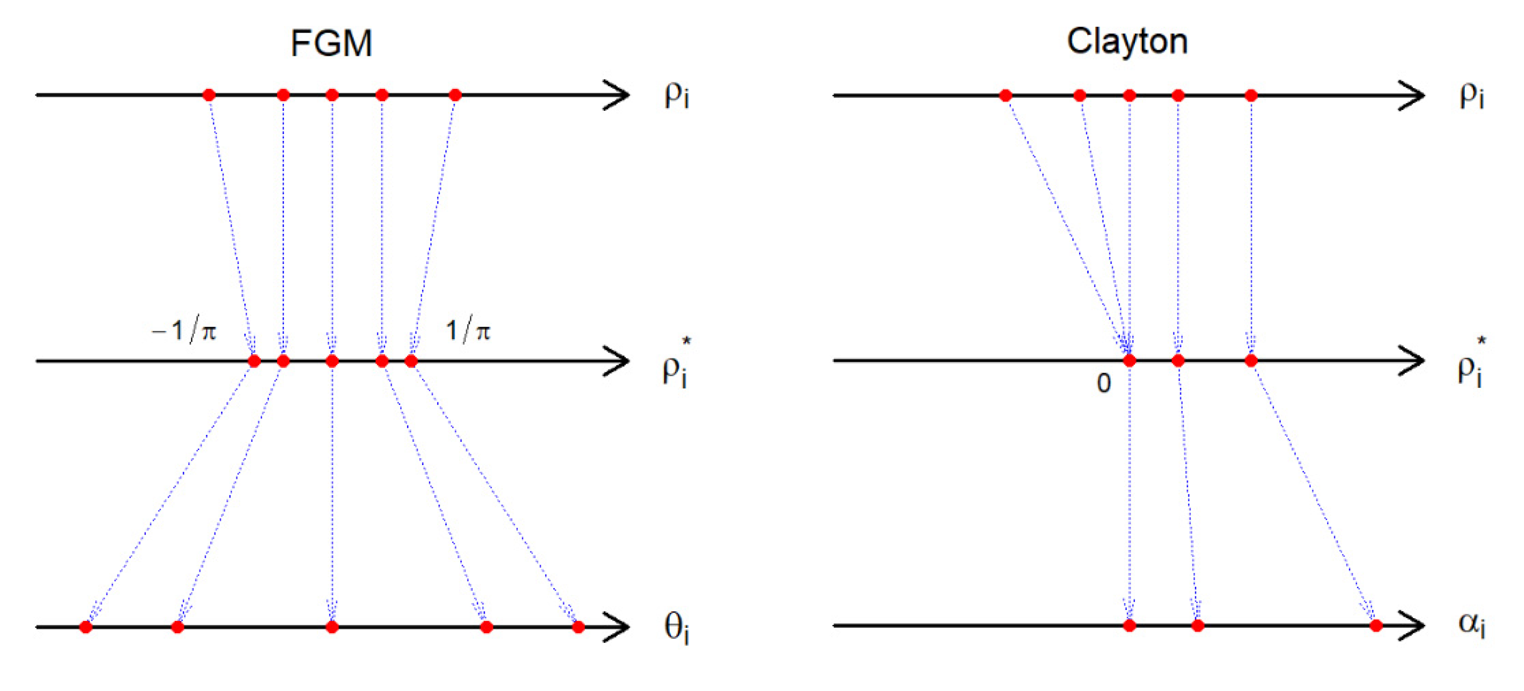
Under this model, the correlation function is ${\rho }_{C^{\mathrm{FGM}}}\left(\theta \right)=\theta /\pi$ for $-1\le \theta \le 1$ [44]. Thus, the copula parameter is identified by ${\theta }_i=\pi {\rho }_i$, as long as ${\rho }_i\in \left[-1/\pi ,1/\pi \left]\approx \right[-0.32,0.32\right]$. If ${\rho }_i\notin \left[-1/\pi ,1/\pi \right]$, we suggest ${\theta }_i=-1$ or ${\theta }_i=1$, using ${\theta }_i\equiv \pi {\rho }_i^{\ast }$, where ${\rho }_i^{\ast }=min[-1/\pi ,max\{{\rho }_i,1/\pi \}]$. Hence, ${\theta }_i$ can still be identified by ${\rho }_i$. This boundary enforcement is illustrated in Figure 1.

Example 3.

(The Clayton copula): Under the Clayton copula, the model in Equation (2) becomes

$$Pr(Y_{i1}\le y_1,Y_{i2}\le y_2)={\left\{\Phi {\left(\frac{y_1-{\mu }_1}{{\sigma }_{i1}}\right)}^{-{\alpha }_i}+\Phi {\left(\frac{y_2-{\mu }_2}{{\sigma }_{i2}}\right)}^{-{\alpha }_i}-1\right\}}^{-1/{\alpha }_i}.$$

for ${\alpha }_i>0$. The correlation function does not have a closed-form, and is written as

$${\rho }_{C^{\mathrm{Clayton}}}\left(\alpha \right)=\left(\alpha +1\right){{\displaystyle \int }}_{-\infty }^{\infty }{{\displaystyle \int }}_{-\infty }^{\infty }\frac{z_1{z}_2\phi \left(z_1\right)\phi \left(z_2\right)}{\Phi {(z_1)}^{\alpha +1}\Phi {(z_2)}^{\alpha +1}{\{\Phi {(z_1)}^{-\alpha }+\Phi {(z_2)}^{-\alpha }-1\}}^{1/\alpha +2}}d{z}_{1}d{z}_2.$$

It is known that ${lim}_{\alpha \to 0}{\rho }_{C^{\mathrm{Clayton}}}\left(\alpha \right)=0$ and ${lim}_{\alpha \to \infty }{\rho }_{C^{\mathrm{Clayton}}}\left(\alpha \right)=1$. In addition, if ${\alpha }_2\ge {\alpha }_1$ then $C_{{\alpha }_2}^{\mathrm{Clayton}}\left(u,v\right)\ge C_{{\alpha }_1}^{\mathrm{Clayton}}\left(u,v\right)$ for all $u,v\in \left(0,1\right)$ [45]. Then, we conclude that the range of the correlation is $R_{C^{\mathrm{Clayton}}}=\left(0,1\right)$. Thus, one can identify by solving ${\rho }_{C^{\mathrm{Clayton}}}\left({\alpha }_i\right)={\rho }_i$ numerically if ${\rho }_i>0$. If ${\rho }_i\le 0$ , we suggest the independence model (Figure 1)

$$Pr(Y_{i1}\le y_1,Y_{i2}\le y_2)=\Phi \left(\frac{y_1-{\mu }_1}{{\sigma }_{i1}}\right)\Phi \left(\frac{y_2-{\mu }_2}{{\sigma }_{i2}}\right).$$

Example 4.

(The Gumbel copula): Under the Gumbel copula, the model in Equation (2) becomes

$$Pr(Y_{i1}\le y_1,Y_{i2}\le y_2)=\exp \left(-{\left[{\left\{-\log \Phi \left(\frac{y_1-{\mu }_1}{{\sigma }_{i1}}\right)\right\}}^{{\beta }_i}+{\left\{-\log \Phi \left(\frac{y_2-{\mu }_2}{{\sigma }_{i2}}\right)\right\}}^{{\beta }_i}\right]}^{1/{\beta }_i}\right)$$

for ${\beta }_i\ge 1$. Similar to the Clayton copula, the correlation function does not have a closed-form, and is not displayed here. It is known that ${\rho }_{C^{\mathrm{Gumbel}}}\left(1\right)=0$ and ${lim}_{\beta \to \infty }{\rho }_{C^{\mathrm{Gumbel}}}\left(\beta \right)=1$. If ${\rho }_i<0$ , we suggest the independence model as in the Clayton copula.

Example 5.

(The Frank copula): Under the Frank copula, the model in Equation (2) becomes

$$Pr(Y_{i1}\le y_1,Y_{i2}\le y_2)=-\frac{1}{{\gamma }_i}\log \left(1+\frac{\left[\exp \left\{-{\gamma }_i\Phi \left(\frac{y_1-{\mu }_1}{{\sigma }_{i1}}\right)\right\}-1\right]\left[\exp \left\{-{\gamma }_i\Phi \left(\frac{y_2-{\mu }_2}{{\sigma }_{i2}}\right)\right\}-1\right]}{e^{-{\gamma }_i}-1}\right)$$

for ${\gamma }_i\ne 0$. Again, the correlation function does not have a closed-form, and is not displayed here. It is known that ${lim}_{\gamma \to -\infty }{\rho }_{C^{\mathrm{Frank}}}\left(\gamma \right)=-1$ and ${lim}_{\gamma \to \infty }{\rho }_{C^{\mathrm{Frank}}}\left(\gamma \right)=1$. Thus, the Frank copula parameter does not require boundary correction.

3.2. Statistical Inference Methods

This subsection develops statistical inference methods under the proposed model.

We propose the MLE for $\mathit{\mu }$ under the general copula model (Definition 1) in Equation (2). Suppose that the copula density $C_{\mathit{\theta }}^{\left[1,1\right]}$ exists. Then, the joint density of ${\mathit{Y}}_i$ is

$$f_{i,\mathit{\mu }}^{}\left(\mathit{y}\right)=\frac{{\partial }^2}{\partial y_1\partial y_2}Pr(Y_{i1}\le y_1,Y_{i2}\le y_2)=\frac{1}{{\sigma }_{i1}{\sigma }_{i2}}\phi \left(\frac{y_1-{\mu }_1}{{\sigma }_{i1}}\right)\phi \left(\frac{y_2-{\mu }_2}{{\sigma }_{i2}}\right)C_{{\mathit{\theta }}_i}^{\left[1,1\right]}\left\{\Phi \left(\frac{Y_1-{\mu }_1}{{\sigma }_{i1}}\right),\Phi \left(\frac{Y_2-{\mu }_2}{{\sigma }_{i2}}\right)\right\}.$$

where $\mathit{y}=\left(y_1,y_2\right)$ and $\phi \left(\cdot \right)$ is the density of $N\left(0,1\right)$. Given the samples, the log-likelihood function is

$${\ell }_n\left(\mathit{\mu }\right)=\mathrm{constant}+{\displaystyle \sum }_{i=1}^n\log \left[C_{{\mathit{\theta }}_i}^{\left[1,1\right]}\left\{\Phi \left(\frac{Y_{i1}-{\mu }_1}{{\sigma }_{i1}}\right),\Phi \left(\frac{Y_{i2}-{\mu }_2}{{\sigma }_{i2}}\right)\right\}\right]-\frac{1}{2}{\displaystyle \sum }_{j=1}^2{\displaystyle \sum }_{i=1}^n{\left(\frac{Y_{ij}-{\mu }_j}{{\sigma }_{ij}}\right)}^2.$$

The MLE of the common mean vector is defined as

$${\widehat{\mathit{\mu }}}_n=\left[\begin{array}{c}{\widehat{\mu }}_{n,1}\\ {\widehat{\mu }}_{n,2}\end{array}\right]=\underset{\mathit{\mu }\in R^2}{\mathrm{argmax}}{\ell }_n\left(\mathit{\mu }\right),$$

where $R=\left(-\infty ,\infty \right)$ is a real line. The MLE does not have a closed-form expression except for the normal copula. Thus, the MLE can also be obtained by the Newton–Raphson algorithm or some software functions (e.g., the R functions optim or nlm). One may also apply our R package CommonMean.Copula [26], which will be explained in Section 6.

3.3. Information Matrix

For the MLE to be well-behaved, it is necessary to show that the (Fisher) information matrix exists and is non-singular. In other words, the MLE, without verifying these conditions, may have some problems, e.g., the non-existence, inconsistency, or inefficiency of the MLE. Furthermore, the information matrix describes how a copula influences the MLE.

We define the $2\times 2$ information matrix $I_i\left(\mathit{\mu }\right)$ for $i=1,2,\dots ,n$ as

$$I_{i,jk}\left(\mathit{\mu }\right)=E\left\{\frac{\partial \log f_{i,\mathit{\mu }}({\mathit{Y}}_i)}{\partial {\mu }_j}\frac{\partial \log f_{i,\mathit{\mu }}({\mathit{Y}}_i)}{\partial {\mu }_k}\right\}, j,k=1,2.$$

The following theorem gives the formula of the information matrix.

Lemma 1.

If$C_{\mathit{\theta }}^{\left[3,1\right]}$,$C_{\mathit{\theta }}^{\left[1,3\right]}$, and$C_{\mathit{\theta }}^{\left[2,2\right]}$exist in${(0,1)}^2$, for each$i$, the following equalities hold

$$E\left\{\frac{\partial \log f_{i,\mathit{\mu }}({\mathit{Y}}_i)}{\partial {\mu }_j}\frac{\partial \log f_{i,\mathit{\mu }}({\mathit{Y}}_i)}{\partial {\mu }_k}\right\}=E\left\{-\frac{{\partial }^2\log f_{i,\mathit{\mu }}({\mathit{Y}}_i)}{\partial {\mu }_j\partial {\mu }_k}\right\}; j,k=1,2.$$

The proof of Lemma 1 is given in Appendix A.1.

Many copulas have $C_{\mathit{\theta }}^{\left[3,1\right]}$, $C_{\mathit{\theta }}^{\left[1,3\right]}$, and $C_{\mathit{\theta }}^{\left[2,2\right]}$ in ${(0,1)}^2$, such as the normal, FGM, and Clayton copulas (Appendix A.2.). The following theorem gives the formula of the information matrix.

Theorem 1.

Under the copula-based model (Definition 1), the information matrix does not depend on$\mathit{\mu }$. Furthermore, if$C_{\mathit{\theta }}^{\left[3,1\right]}$,$C_{\mathit{\theta }}^{\left[1,3\right]}$, and$C_{\mathit{\theta }}^{\left[2,2\right]}$exist in${(0,1)}^2$, it can be decomposed into the sum of the information matrix for the independent model and the additional information by the copula,

$$I_i=\left[\begin{array}{cc}\frac{1}{{\sigma }_{i1}^2}& 0\\ 0& \frac{1}{{\sigma }_{i2}^2}\end{array}\right]+\left[\begin{array}{cc}\frac{1}{{\sigma }_{i1}^2}{E}_C^{11}\left({\mathit{\theta }}_i\right)& \frac{1}{{\sigma }_{i1}{\sigma }_{i2}}\left\{E_C^{12}\left({\mathit{\theta }}_i\right)-{\rho }_C\left({\mathit{\theta }}_i\right)\right\}\\ \frac{1}{{\sigma }_{i1}{\sigma }_{i2}}\left\{E_C^{12}\left({\mathit{\theta }}_i\right)-{\rho }_C\left({\mathit{\theta }}_i\right)\right\}& \frac{1}{{\sigma }_{i2}^2}{E}_C^{22}\left({\mathit{\theta }}_i\right)\end{array}\right],$$

(3)

where

$$E_C^{11}\left({\mathit{\theta }}_i\right)=E{\left\{\frac{\phi \left(Z_{i1}\right)C_{{\mathit{\theta }}_i}^{\left[2,1\right]}\left\{\Phi \left(Z_{i1}\right),\Phi \left(Z_{i2}\right)\right\}}{C_{{\mathit{\theta }}_i}^{\left[1,1\right]}\left\{\Phi \left(Z_{i1}\right),\Phi \left(Z_{i2}\right)\right\}}\right\}}^2,$$

$$E_C^{22}\left({\mathit{\theta }}_i\right)=E{\left\{\frac{\phi \left(Z_{i2}\right)C_{{\mathit{\theta }}_i}^{\left[1,2\right]}\left\{\Phi \left(Z_{i1}\right),\Phi \left(Z_{i2}\right)\right\}}{C_{{\mathit{\theta }}_i}^{\left[1,1\right]}\left\{\Phi \left(Z_{i1}\right),\Phi \left(Z_{i2}\right)\right\}}\right\}}^2,$$

$$E_C^{12}\left({\mathit{\theta }}_i\right)=E\left[\frac{\phi \left(Z_{i1}\right)\phi \left(Z_{i2}\right)C_{{\mathit{\theta }}_i}^{\left[2,1\right]}\left\{\Phi \left(Z_{i1}\right),\Phi \left(Z_{i2}\right)\right\}{C}_{{\mathit{\theta }}_i}^{\left[1,2\right]}\left\{\Phi \left(Z_{i1}\right),\Phi \left(Z_{i2}\right)\right\}}{C_{{\mathit{\theta }}_i}^{\left[1,1\right]}{\{\Phi \left(Z_{i1}\right),\Phi \left(Z_{i2}\right)\}}^2}\right].$$

Theorem 1 can be proved by straightforward calculations as Lemma 1 (Appendix A.1.). Theorem 1 helps us interpret the role of the copula $C_{{\mathit{\theta }}_i}$ on the information matrix.

Theorem 2.

The determinant of$I_i$can be expressed as

$$\begin{gathered} \det (I_i)=\frac{1}{{\sigma }_{i1}^2{\sigma }_{i2}^2}\{E_C^{11}\left({\mathit{\theta }}_i\right)E_C^{22}\left({\mathit{\theta }}_i\right)-E_C^{12}{({\mathit{\theta }}_i)}^2\} \\ +\frac{1}{{\sigma }_{i1}^2{\sigma }_{i2}^2}\{E_C^{11}\left({\mathit{\theta }}_i\right)+E_C^{22}\left({\mathit{\theta }}_i\right)+2{\rho }_C\left({\mathit{\theta }}_i\right)E_C^{12}({\mathit{\theta }}_i)\}+\frac{1}{{\sigma }_{i1}^2{\sigma }_{i2}^2}\{1-{\rho }_C{({\mathit{\theta }}_i)}^2\}. \end{gathered}$$

In addition,$\det (I_i)>0$and$I_i$is positive definite.

Proof of Theorem 2.

The expression of $\det (I_i)$ is obtained by straightforward calculations. Clearly, we have $\left|{\rho }_C\left({\mathit{\theta }}_i\right)\right|<1$. Then, by the Cauchy-Schwarz inequality,

$$E_C^{11}\left({\mathit{\theta }}_i\right)E_C^{22}\left({\mathit{\theta }}_i\right)\ge E_C^{12}{({\mathit{\theta }}_i)}^2.$$

Furthermore, by the arithmetic-geometric mean inequality, we have

$$E_C^{11}\left({\mathit{\theta }}_i\right)+E_C^{22}\left({\mathit{\theta }}_i\right)\ge 2{\left\{E_C^{11}\left({\mathit{\theta }}_i\right)E_C^{22}\left({\mathit{\theta }}_i\right)\right\}}^{1/2}\ge 2\left|E_C^{12}\left({\mathit{\theta }}_i\right)\right|>2\left|{\rho }_C\left({\mathit{\theta }}_i\right)E_C^{12}\left({\mathit{\theta }}_i\right)\right|.$$

Then we obtain $\det (I_i)>0$. Since $E_C^{11}\left({\mathit{\theta }}_i\right)/{\sigma }_{i1}^2+1/{\sigma }_{i1}^2>0$, both the upper left $1\times 1$ and $2\times 2$ determinants of $I_i$ are positive. Thus, $I_i$ is positive definite. □

Based on Theorem 1, one can derive the information matrix $I_i\left(\mathit{\mu }\right)$ for parametric copulas. Below, we show examples of the normal, FGM, and Clayton copulas.

Example 6.

(The normal copula): Under the normal copula

$$E_{C^{\mathrm{Normal}}}^{11}\left({\rho }_i\right)=E_{C^{\mathrm{Normal}}}^{22}\left({\rho }_i\right)=\frac{{\rho }_i^2}{1-{\rho }_i^2}, E_{C^{\mathrm{Normal}}}^{12}\left({\rho }_i\right)=-\frac{{\rho }_i^3}{1-{\rho }_i^2}.$$

Then, by Theorem 1, the information matrix in Equation (3) becomes

$$\begin{gathered} I_i=\left[\begin{array}{cc}\frac{1}{{\sigma }_{i1}^2}& 0\\ 0& \frac{1}{{\sigma }_{i2}^2}\end{array}\right]+\left[\begin{array}{cc}\frac{1}{{\sigma }_{i1}^2}\frac{{\rho }_i^2}{1-{\rho }_i^2}& \frac{1}{{\sigma }_{i1}{\sigma }_{i2}}\left(-\frac{{\rho }_i^3}{1-{\rho }_i^2}-{\rho }_i\right)\\ \frac{1}{{\sigma }_{i1}{\sigma }_{i2}}\left(-\frac{{\rho }_i^3}{1-{\rho }_i^2}-{\rho }_i\right)& \frac{1}{{\sigma }_{i2}^2}\frac{{\rho }_i^2}{1-{\rho }_i^2}\end{array}\right] \\ =\frac{1}{1-{\rho }_i^2}\left[\begin{array}{cc}\frac{1}{{\sigma }_{i1}^2}& -\frac{{\rho }_i}{{\sigma }_{i1}{\sigma }_{i2}}\\ -\frac{{\rho }_i}{{\sigma }_{i1}{\sigma }_{i2}}& \frac{1}{{\sigma }_{i2}^2}\end{array}\right]={\mathit{\Omega }}_i^{-1}. \end{gathered}$$

and its determinant is $\det (I_i^{\mathrm{Normal}})=1/\left({\sigma }_{i1}^2{\sigma }_{i2}^2\right)$. Clearly, $I_i^{\mathrm{Normal}}$ is positive definite.

Example 7.

(The FGM copula): Under the FGM copula

$$E_{C^{\mathrm{FGM}}}^{11}\left({\theta }_i\right)=E_{C^{\mathrm{FGM}}}^{22}\left({\theta }_i\right)=4{\theta }_i^2{{\displaystyle \int }}_{-\infty }^{\infty }{{\displaystyle \int }}_{-\infty }^{\infty }\frac{\phi {\left(z_1\right)}^3{\{1-2\Phi \left(z_2\right)\}}^2\phi \left(z_2\right)}{1+{\theta }_i\left\{1-2\Phi \left(z_1\right)\right\}\left\{1-2\Phi \left(z_2\right)\right\}}d{z}_{1}d{z}_2,$$

$$E_{C^{\mathrm{FGM}}}^{12}\left({\theta }_i\right)=4{\theta }_i^2{{\displaystyle \int }}_{-\infty }^{\infty }{{\displaystyle \int }}_{-\infty }^{\infty }\frac{\phi {\left(z_1\right)}^2\left\{1-2\Phi \left(z_1\right)\right\}\phi {\left(z_2\right)}^2\left\{1-2\Phi \left(z_2\right)\right\}}{1+{\theta }_i\left\{1-2\Phi \left(z_1\right)\right\}\left\{1-2\Phi \left(z_2\right)\right\}}d{z}_{1}d{z}_2, {\rho }_{C^{\mathrm{FGM}}}\left(\theta \right)=\frac{\theta }{\pi }.$$

Then, by Theorem 1, the information matrix in Equation (3) becomes

$$I_i^{\mathrm{FGM}}=\left[\begin{array}{cc}\frac{1}{{\sigma }_{i1}^2}& 0\\ 0& \frac{1}{{\sigma }_{i2}^2}\end{array}\right]+\left[\begin{array}{cc}\frac{1}{{\sigma }_{i1}^2}{E}_{C^{\mathrm{FGM}}}^{11}\left({\theta }_i\right)& \frac{1}{{\sigma }_{i1}{\sigma }_{i2}}{E}_{C^{\mathrm{FGM}}}^{12}\left({\theta }_i\right)-\frac{{\theta }_i}{\pi {\sigma }_{i1}{\sigma }_{i2}}\\ \frac{1}{{\sigma }_{i1}{\sigma }_{i2}}{E}_{C^{\mathrm{FGM}}}^{12}\left({\theta }_i\right)-\frac{{\theta }_i}{\pi {\sigma }_{i1}{\sigma }_{i2}}& \frac{1}{{\sigma }_{i2}^2}{E}_{C^{\mathrm{FGM}}}^{22}\left({\theta }_i\right)\end{array}\right].$$

By Theorem 2, its determinant is

$$\begin{gathered} \det (I_i)=\frac{1}{{\sigma }_{i1}^2{\sigma }_{i2}^2}\left\{E_{C^{\mathrm{FGM}}}^{11}{\left({\theta }_i\right)}^2-E_{C^{\mathrm{FGM}}}^{12}{\left({\theta }_i\right)}^2\right\} \\ +\frac{2}{{\sigma }_{i1}^2{\sigma }_{i2}^2}\left\{E_{C^{\mathrm{FGM}}}^{11}\left({\theta }_i\right)+\frac{{\theta }_i}{\pi }{E}_{C^{\mathrm{FGM}}}^{12}\left({\theta }_i\right)\right\}+\frac{1}{{\sigma }_{i1}^2{\sigma }_{i2}^2}\left(1-\frac{{\theta }_i^2}{{\pi }^2}\right). \end{gathered}$$

This result agrees with [3] who considered the FGM model.

Example 8.

(The Clayton copula): Under the Clayton copula

$$E_{C^{\mathrm{Clayton}}}^{11}\left({\alpha }_i\right)=E_{C^{\mathrm{Clayton}}}^{22}\left({\alpha }_i\right)=\left({\alpha }_i+1\right){{\displaystyle \int }}_{-\infty }^{\infty }{{\displaystyle \int }}_{-\infty }^{\infty }\frac{\phi {(z_1)}^3\phi \left(z_2\right){\{{\alpha }_i\Phi {(z_1)}^{-{\alpha }_i}-\left({\alpha }_i+1\right)\Phi {(z_2)}^{-{\alpha }_i}+\left({\alpha }_i+1\right)\}}^2}{\Phi {(z_1)}^{{\alpha }_i+3}\Phi {(z_2)}^{{\alpha }_i+1}{\{\Phi {(z_1)}^{-{\alpha }_i}+\Phi {(z_2)}^{-{\alpha }_i}-1\}}^{1/{\alpha }_i+4}}d{z}_{1}d{z}_2,$$

$$\begin{gathered} E_{C^{\mathrm{Clayton}}}^{12}\left({\alpha }_i\right)={{\displaystyle \int }}_{-\infty }^{\infty }{{\displaystyle \int }}_{-\infty }^{\infty }\frac{\phi {(z_1)}^2\{{\alpha }_i\Phi {(z_1)}^{-{\alpha }_i}-\left({\alpha }_i+1\right)\Phi {(z_2)}^{-{\alpha }_i}+\left({\alpha }_i+1\right)\}}{\Phi {(z_1)}^{{\alpha }_i+2}{\{\Phi {(z_1)}^{-{\alpha }_i}+\Phi {(z_2)}^{-{\alpha }_i}-1\}}^{1/2{\alpha }_i+2}} \\ \times \frac{\phi {(z_2)}^2\{{\alpha }_i\Phi {(z_2)}^{-{\alpha }_i}-\left({\alpha }_i+1\right)\Phi {(z_1)}^{-{\alpha }_i}+\left({\alpha }_i+1\right)\}}{\Phi {(z_2)}^{{\alpha }_i+2}{\{\Phi {(z_1)}^{-{\alpha }_i}+\Phi {(z_2)}^{-{\alpha }_i}-1\}}^{1/2{\alpha }_i+2}}d{z}_{1}d{z}_2, \end{gathered}$$

$${\rho }_{C^{\mathrm{Clayton}}}\left({\alpha }_i\right)=\left({\alpha }_i+1\right){{\displaystyle \int }}_{-\infty }^{\infty }{{\displaystyle \int }}_{-\infty }^{\infty }\frac{z_1{z}_2\phi \left(z_1\right)\phi \left(z_2\right)}{\Phi {(z_1)}^{{\alpha }_i+1}\Phi {(z_2)}^{{\alpha }_i+1}{\{\Phi {(z_1)}^{-{\alpha }_i}+\Phi {(z_2)}^{-{\alpha }_i}-1\}}^{1/{\alpha }_i+2}}d{z}_{1}d{z}_2.$$

Then, by Theorems 1 and 2, we obtain$I_i^{\mathrm{Clayton}}$and$\det (I_i^{\mathrm{Clayton}})$accordingly.

4. Asymptotic Theory

To assess the sampling variability of ${\widehat{\mathit{\mu }}}_n$, its asymptotic distribution is presented in this section.

A technical burden comes from the fact that our samples ${\mathit{Y}}_i$, $i=1,2,\dots ,n$ are independent and non-identically distributed (i.n.i.d.) owing to heterogeneous variances (${\mathit{\Omega }}_i\ne {\mathit{\Omega }}_j,i\ne j$). The existence of the asymptotic distribution requires the stabilization of the information matrix [3,46,47] in large samples. For the asymptotic variance of ${\widehat{\mathit{\mu }}}_n$, to be defined, we assume the existence of a $2\times 2$ positive definite matrix $I\equiv {\lim }_{n\to \infty }{{\displaystyle \sum }}_{i=1}^n{I}_i/n$. We further assume that the copula’s derivatives $C_{\mathit{\theta }}^{\left[4,1\right]}$, $C_{\mathit{\theta }}^{\left[3,2\right]}$, $C_{\mathit{\theta }}^{\left[2,3\right]}$, and $C_{\mathit{\theta }}^{\left[1,4\right]}$ exist in ${(0,1)}^2$. With these conditions and many other technical conditions given in [48], we establish the consistency and asymptotic normality of ${\widehat{\mathit{\mu }}}_n$:

Theorem 3.

Under the copula model (Definition 1), if some regularity conditions hold, then

(a) 

Existence and consistency: With probability tending to one, there exists the MLE${\widehat{\mathit{\mu }}}_n=\left({\widehat{\mu }}_{n,1},{\widehat{\mu }}_{n,2}\right)$such that${\widehat{\mathit{\mu }}}_n{\to }^p\mathit{\mu }$, as$n\to \infty$;

(b) 

Asymptotic normality:$n^{1/2}\left({\widehat{\mathit{\mu }}}_n-\mathit{\mu }\right){\to }^{d}N\left(0,I^{-1}\right)$, as$n\to \infty$.

The proof of Theorem 3 and the required regularity conditions are given in the Ph.D dissertation of [48]. The proof approximates $n^{1/2}\left({\widehat{\mathit{\mu }}}_n-\mathit{\mu }\right)$ by the sum of independent random variables, and then applies the weak law of large numbers for i.n.i.d. random variables from Theorem 1.14 in [49] and the Lindeberg–Feller multivariate central limit theorem from Proposition 2.27 in [50]. The proof is fairly technical, but similar to those of Theorem 6.5.1 in [51], Theorem 1 in [47], and Theorem 5.1 in [3].

5. SE and Confidence Sets

As Section 4 has established the asymptotic theory to evaluate the variability of the proposed MLE, we can derive the SE, confidence interval (CI), and confidence ellipse (CE).

Let $g:R^2\mapsto R$ be a differentiable function, and $g\left(\mathit{\mu }\right)$ be the parameter of interest. For instance, $g\left(\mathit{\mu }\right)={\mu }_1$ and $g\left(\mathit{\mu }\right)={\mu }_2-{\mu }_1$ can be considered. The SE of $g\left({\widehat{\mathit{\mu }}}_n\right)$ is

$$\mathrm{SE}\left\{g\left({\widehat{\mathit{\mu }}}_n\right)\right\}={\left[{\left.{\left\{\frac{\partial g\left(\mathit{\mu }\right)}{\partial \mathit{\mu }}\right\}}^T{\left\{-\frac{{\partial }^2{\ell }_n\left(\mathit{\mu }\right)}{\partial \mathit{\mu }\partial {\mathit{\mu }}^T}\right\}}^{-1}\left\{\frac{\partial g\left(\mathit{\mu }\right)}{\partial \mathit{\mu }}\right\}\right|}_{\mathit{\mu }={\widehat{\mathit{\mu }}}_n}\right]}^{1/2}.$$

This formula is based on the delta method and the large sample approximation

$$I\approx \frac{1}{n}{\displaystyle \sum }_{i=1}^n{I}_i\approx {\left.-\frac{1}{n}\frac{{\partial }^2{\ell }_n\left(\mathit{\mu }\right)}{\partial \mathit{\mu }\partial {\mathit{\mu }}^T}\right|}_{\mathit{\mu }={\widehat{\mathit{\mu }}}_n}.$$

The 95% CI for $g\left(\mathit{\mu }\right)$ is $g\left({\widehat{\mathit{\mu }}}_n\right)\pm 1.96\times \mathrm{SE}\left\{g\left({\widehat{\mathit{\mu }}}_n\right)\right\}$.

Moreover, based on Theorem 3, we construct a 95% CE for $\mathit{\mu }$:

$$\mathrm{CE}=\left\{\mathit{\mu }:{({\widehat{\mathit{\mu }}}_n-\mathit{\mu })}^T\left({\left.-\frac{{\partial }^2{\ell }_n\left(\mathit{\mu }\right)}{\partial \mathit{\mu }\partial {\mathit{\mu }}^T}\right|}_{\mathit{\mu }={\widehat{\mathit{\mu }}}_n}\right)\left({\widehat{\mathit{\mu }}}_n-\mathit{\mu }\right)\le {\chi }_{\mathrm{df}=2,0.95}^2\right\},$$

where ${\chi }_{\mathrm{df}=2,0.95}^2$ is be the 95% point of the ${\chi }^2$-distribution with two degrees of freedom.

6. R Package

We implement the proposed methods in an R package CommonMean.Copula [26]. R users can easily compute the MLE with its SE and 95% CI under the FGM, Clayton, Gumbel, Frank, and normal copulas. In this package, the log-likelihood is maximized by the R optim function, where the initial values are set as the univariate estimators

$${\mu }_j^{\left(0\right)}={\left({\displaystyle \sum }_{i=1}^n\frac{1}{{\sigma }_{ij}^2}\right)}^{-1}{\displaystyle \sum }_{i=1}^n\frac{Y_{ij}}{{\sigma }_{ij}^2}, j=1,2.$$

For illustration, we fitted the Clayton copula by the following R codes:

- some outputs are omitted for brevity –

Here, $CommonMean1 shows ${\widehat{\mu }}_{n,1}^{\mathrm{Clayton}}=33.95$, $\mathrm{SE}({\widehat{\mu }}_{n,1}^{\mathrm{Clayton}})=0.439$, and the 95% CI (33.089, 34.812); $CommonMean2 is similar. $V shows the covariance matrix $Cov({\widehat{\mathit{\mu }}}_n^{\mathrm{Clayton}})$. $‘Log-likelihood values’ shows ${\ell }_n^{\mathrm{Clayton}}({\widehat{\mathit{\mu }}}_n^{\mathrm{Clayton}})=-285.65$. One can fit other copulas by changing “Clayton” to “FGM”, “Gumbel”, “Frank”, or “normal”.

7. Simulation Studies

We conducted Monte Carlo simulations to examine the accuracy of the proposed methods. We report the results for the Clayton copula; more results are available from [48].

We generated ${\mathit{Y}}_i$, $i=1,2,\dots ,n$, under the Clayton copula with ${\alpha }_i~Gamma\left(64,1/8\right)$, $Gamma\left(4,1/2\right)$, or $Gamma\left(1,1\right)$, leading to $E\left[{\alpha }_i\right]=8$, $E\left[{\alpha }_i\right]=2$, or $E\left[{\alpha }_i\right]=1$, respectively. In all three cases, we have $Var\left[{\alpha }_i\right]=1$. Without loss of generality, we set $\mathit{\mu }=\left(0,0\right)$. To set ${\sigma }_{i1}^2$ and ${\sigma }_{i2}^2$, we followed the simulation setting of [52]. That is, ${\sigma }_{i1}^2,{\sigma }_{i2}^2~{\chi }_{df=1}^2/4$, restricted in the interval $\left[0.009,0.6\right]$. This setting leads to $E\left[{\sigma }_{i1}^2\left]=E\right[{\sigma }_{i2}^2\right]=0.173$. Based on the generated data, we computed ${\widehat{\mu }}_{n,1}^{\mathrm{Clayton}}$, ${\widehat{\mu }}_{n,2}^{\mathrm{Clayton}}-{\widehat{\mu }}_{n,1}^{\mathrm{Clayton}}$, and ${\widehat{\mathit{\mu }}}_n^{\mathrm{Clayton}}$, and their SEs and 95% CIs (CEs) by using the R function CommonMean.Copula (Section 6). We then evaluated the coverage probability (CP) of the 95% CI (CE) to see how the confidence set can cover the true value. We consider a small sample size $n\in \left\{5,10,15\right\}$ and a large sample size $n\in \left\{50,100,300\right\}$. Our simulations are based on 1000 repetitions.

Table 1. Simulation results based on 1000 repetitions.

		${\widehat{\mathit{\mu }}}_{\mathit{n},1}^{\mathbf{Clayton}}$			${\widehat{\mathit{\mu }}}_{\mathit{n},2}^{\mathbf{Clayton}}-{\widehat{\mathit{\mu }}}_{\mathit{n},1}^{\mathbf{Clayton}}$			${\widehat{\mathit{\mu }}}_{\mathit{n}}^{\mathbf{Clayton}}$
Parameters	$\mathit{n}$	SD	SE	CP	SD	SE	CP	CP
$E\left[{\alpha }_i\right]=8$	5	0.064	0.046	0.888	0.042	0.033	0.885	0.859
	10	0.033	0.026	0.913	0.023	0.019	0.931	0.894
	15	0.021	0.019	0.933	0.015	0.014	0.936	0.919
	50	0.010	0.009	0.952	0.007	0.007	0.954	0.950
	100	0.007	0.006	0.955	0.005	0.005	0.943	0.944
	300	0.004	0.004	0.948	0.003	0.003	0.942	0.948
$E\left[{\alpha }_i\right]=2$	5	0.105	0.092	0.938	0.100	0.086	0.920	0.909
	10	0.061	0.057	0.937	0.060	0.055	0.929	0.919
	15	0.049	0.045	0.938	0.045	0.042	0.943	0.930
	50	0.023	0.023	0.959	0.022	0.021	0.944	0.943
	100	0.016	0.016	0.942	0.015	0.015	0.957	0.950
	300	0.009	0.009	0.946	0.008	0.008	0.946	0.949
$E\left[{\alpha }_i\right]=1$	5	0.115	0.105	0.932	0.128	0.120	0.935	0.922
	10	0.069	0.068	0.950	0.079	0.075	0.937	0.937
	15	0.058	0.053	0.941	0.062	0.058	0.947	0.937
	50	0.028	0.027	0.942	0.029	0.030	0.955	0.943
	100	0.019	0.019	0.942	0.021	0.020	0.936	0.945
	300	0.010	0.011	0.958	0.011	0.012	0.960	0.959

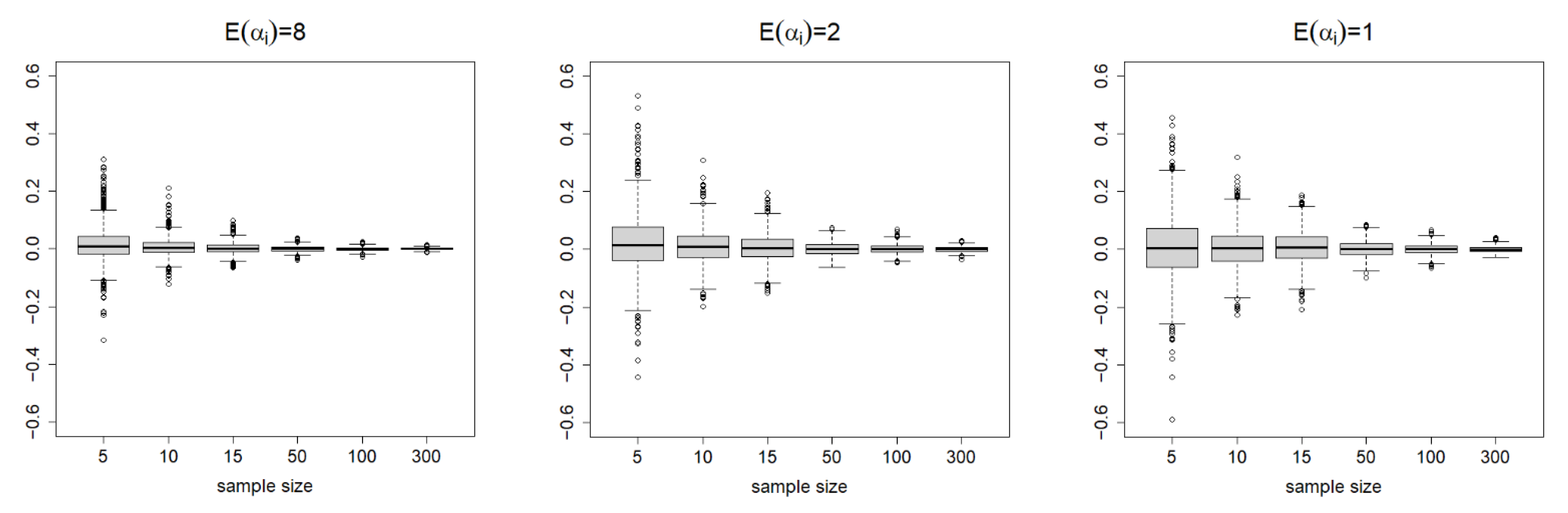
SD = standard deviation, SE = standard error, CP = coverage probability of the 95% CI (CE).

summarizes the results. For ${\widehat{\mu }}_{n,1}^{\mathrm{Clayton}}$ and ${\widehat{\mu }}_{n,2}^{\mathrm{Clayton}}-{\widehat{\mu }}_{n,1}^{\mathrm{Clayton}}$, the SDs of the estimates decrease when $n$ increases from $n=5$ to $n=300$. We report the boxplots summarizing the 1000 repetitions for ${\widehat{\mu }}_{n,1}^{\mathrm{Clayton}}$ in Figure 2. This clearly visualizes how the variability of the estimates vanishes as the sample sizes increase. Table 1 also shows that the SDs are close to the average SEs, except for $n=5$ (due to the very small samples). Consequently, the CPs are close enough to the nominal level of 0.95, especially when sample sizes are large, which is consistent with our asymptotic theories. For ${\widehat{\mathit{\mu }}}_n^{\mathrm{Clayton}}$, the CPs of the 95% CEs are also reasonably close to the nominal level. In summary, the proposed estimators and the asymptotic theory work fairly well in finite samples.

8. Data Analysis

We analyze two real datasets to illustrate the usefulness of the proposed methods.

8.1. The Entrance Exam Data

The first dataset we analyzed was the entrance exam scores on mathematics and statistics, which was introduced by [3]. The data come from undergrad students who took written exams from 2013 to 2017 to enter the Graduate Institute of Statistics, National Central University, Taiwan. The possible score range is from 0 to 100 for both subjects. Let $i=1,2,\dots ,5$ be indices for years 2013, 2014, …, 2017.

Table 2. The entrance exam data from [3].

$\mathit{i}$	Year	Mean Math Score $\left({\mathit{Y}}_{\mathit{i}1}\right)$	Mean Stat Score $\left({\mathit{Y}}_{\mathit{i}2}\right)$	Covariance Matrix $\left({\mathit{\Omega }}_{\mathit{i}}\right)$	Copula Parameter
					${\mathit{\rho }}_{\mathit{i}}$	${\mathit{\theta }}_{\mathit{i}}$	${\mathit{\alpha }}_{\mathit{i}}$	${\mathit{\beta }}_{\mathit{i}}$	${\mathit{\gamma }}_{\mathit{i}}$
1	2013	35.17	30.41	$\left[\begin{array}{cc}1.77& 0.89\\ 0.89& 2.99\end{array}\right]$	0.38	1.00	0.67	1.34	2.68
2	2014	23.43	31.63	$\left[\begin{array}{cc}1.89& 1.76\\ 1.76& 3.61\end{array}\right]$	0.67	1.00	1.92	1.90	6.00
3	2015	30.74	48.11	$\left[\begin{array}{cc}2.15& 2.12\\ 2.12& 6.13\end{array}\right]$	0.58	1.00	1.37	1.65	4.67
4	2016	50.91	65.22	$\left[\begin{array}{cc}3.87& 2.91\\ 2.91& 5.02\end{array}\right]$	0.66	1.00	1.82	1.85	5.76
5	2017	61.62	40.22	$\left[\begin{array}{cc}3.17& 2.10\\ 2.10& 3.29\end{array}\right]$	0.65	1.00	1.75	1.83	5.60

${\rho }_i$ = the Pearson correlation; ${\theta }_i$ = the FGM copula parameter; ${\alpha }_i$ = the Clayton copula parameter; ${\beta }_i$ = the Gumbel copula parameter; ${\gamma }_i$ = the Frank copula parameter.

provides the data, including the values of mathematics ($Y_{i1}$ = mean math score) and statistics ($Y_{i2}$ = mean stat score), and their covariance matrix (${\mathit{\Omega }}_i$).

We fitted the data to the proposed model using the R function CommonMean.Copula(.) in our R package (Section 6).

Table 3. Estimation results for the entrance exam data.

Copula	Math: Estimate (95% CI)	Stat: Estimate (95% CI)	Log-likelihood	$\mathit{C}\mathit{V}$
FGM	37.16 (35.85, 38.47)	41.17 (39.65, 42.70)	−291.80	2723.91
Clayton	32.56 (31.71, 33.40)	43.80 (42.55, 45.05)	−322.84	2644.03
Gumbel	37.67 (36.30, 39.03)	42.56 (40.79, 44.33)	−279.28	2860.21
Frank	37.23 (35.97, 38.49)	39.76 (38.13, 41.40)	−287.63	2738.09
Normal	35.83 (34.51, 37.16)	38.64 (36.94, 40.34)	−342.65	2773.41

summarizes the fitted results for the FGM, Clayton, Gumbel, Frank, and normal copulas. According to the values of the log-likelihood, the Gumbel copula produces the best fit, the Frank copula the second best, and the bivariate normal model the worst fit. The FGM copula failed to capture the dependence and fitted at the boundary ${\theta }_i=1$ for all $i$ (Table 2).

Since the number of unknown parameters across different copulas is the same, model selection by the Akaike information criterion (AIC) is equivalent to model selection by the log-likelihood value. An alternative way of selecting a copula is based on a leave-one-out cross validation (CV), defined as

$$CV={\displaystyle \sum }_{i=1}^n\{{\left(Y_{i1}-{\widehat{\mu }}_{n,1}^{\left(-i\right)}\right)}^2+{\left(Y_{i2}-{\widehat{\mu }}_{n,2}^{\left(-i\right)}\right)}^2\},$$

where ${\widehat{\mu }}_{n,1}^{\left(-i\right)}$ and ${\widehat{\mu }}_{n,2}^{\left(-i\right)}$ are the MLE obtained without the ith sample. Here, $CV$ measures how a sample is predicted by the others under a copula model. A smaller $CV$ corresponds to a better performance of the model.

Table 3 reports the values of $CV$ for each copula. It shows that the Clayton copula has the best performance while the Gumbel copula has the worst. The normal copula has the second worst performance. Overall, our analysis clearly shows the insufficiency of the bivariate normal model.

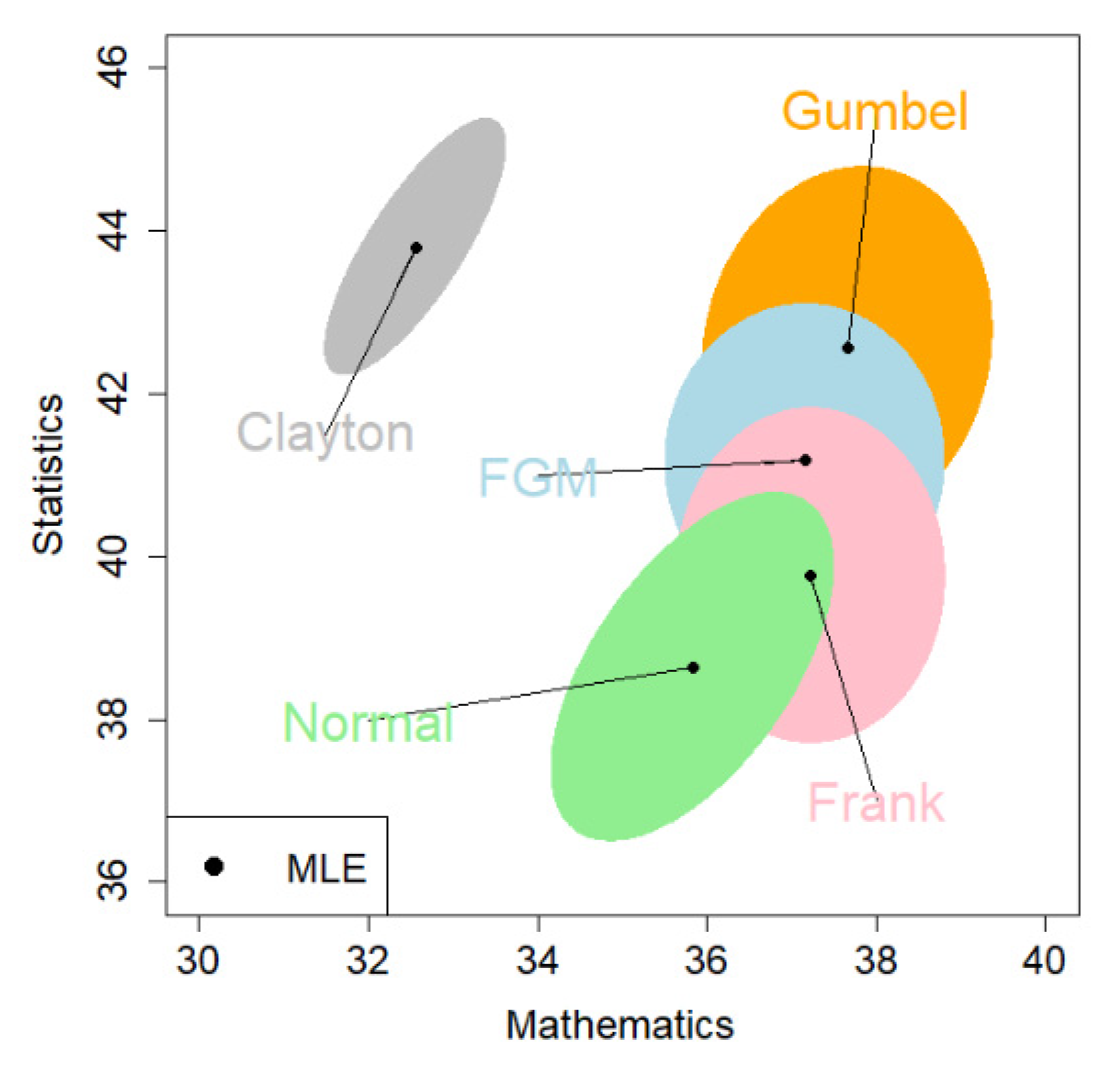
Figure 3 shows the 95% CEs for the mean vector $\mathit{\mu }$. This visualizes how the resultant estimates vary from the choice of copulas. Interestingly, the CE under the Clayton copula is far away from the other four, although it has a larger log-likelihood value than the normal copula. The normal and Clayton copulas produce the rotated oval shape of the CEs, representing a positive dependence between math and stat scores. The FGM and Gumbel copulas produce similar shapes for their CE. We adopt the 95% CE given by the Gumbel copula because it has the largest log-likelihood value.

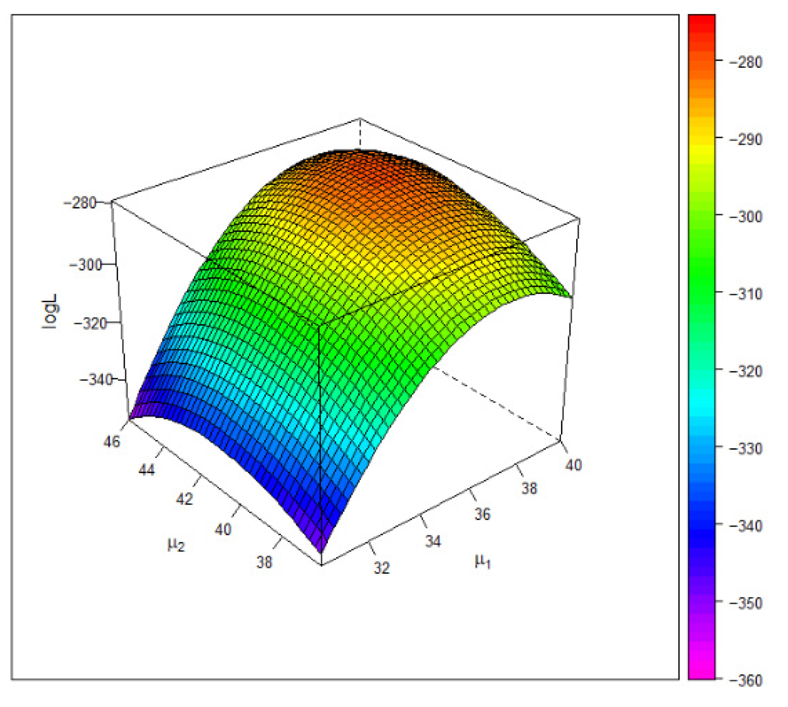
Figure 4 gives the 3D plot of the log-likelihood surface under the Gumbel copula model. The plot shows that the estimate of the common mean ${\widehat{\mathit{\mu }}}_n^{\mathrm{Gumbel}}=\left(37.67,42.56\right)$ attains the global maximum of the log-likelihood function.

8.2. The Blood Pressure Data

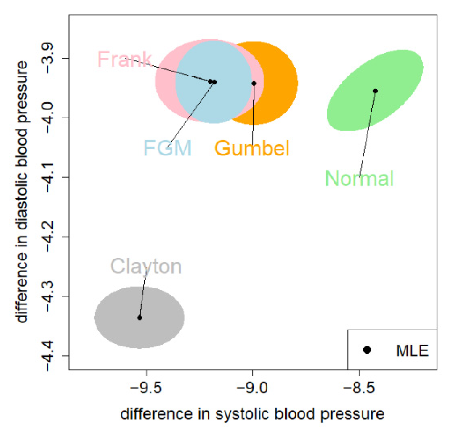
The second dataset we used contains 10 studies that examined the effectiveness of hypertension treatment for lowering blood pressure. Each study provides complete data on two treatment effects, the difference in systolic blood pressure (SBP) and diastolic blood pressure (DBP) between the treatment and the control groups, where these differences are adjusted for the participants’ baseline blood pressures. The within-study correlations of the two outcomes range from ${\rho }_i=0.45$ to ${\rho }_i=0.78$, exhibiting positive dependence. This dataset is available in R package mvmeta [30] and was previously analyzed by [53].

We fitted the data to the proposed copula models using the R function CommonMean.Copula(.) in our R package (Section 6).

Table 4. Estimation results for the blood pressure data.

Copula	SBP: Estimate (95% CI)	DBP: Estimate (95% CI)	Log-likelihood	$\mathit{C}\mathit{V}$
FGM	−9.18 (−9.32, −9.04)	−3.94 (−4.00, −3.89)	−530.29	177.23
Clayton	−9.53 (−9.70, −9.36)	−4.34 (−4.38, −4.29)	−787.02	163.04
Gumbel	−8.99 (−9.16, −8.83)	−3.94 (−4.00, −3.89)	−514.67	184.67
Frank	−9.20 (−9.40, −9.00)	−3.94 (−3.99, −3.88)	−513.34	179.81
Normal	−8.43 (−8.60, −8.25)	−3.95 (−4.01, −3.90)	−771.82	206.49

SBP = the difference in systolic blood pressure; DBP = the difference in diastolic blood pressure.

summarizes the fitted results for all the copulas. Based on the log-likelihood values, the Frank copula produces the best fit, the Gumbel copula the second best, and the Clayton copula produces the worst fit. The FGM copula failed to capture the dependence and fitted at the boundary ${\theta }_i=1$ for all $i$. Again, our analysis reveals the insufficiency of the bivariate normal model; the Frank copula best captured the correlations in the blood pressure data. We also compared $CV$ across all the copulas (Table 4). The results show that the Clayton copula has the best performance while the normal copula has the worst. Again, our analysis shows the insufficiency of the normal model.

Figure 5 shows the 95% CEs for the mean vector $\mathit{\mu }$. The CE under the Clayton and normal copula are far away from the other three. The CE under the FGM copula was almost fully covered by the CE under the Frank copula. We adopt the 95% CE given by the Frank copula, since it has the largest log-likelihood value (Table 4).

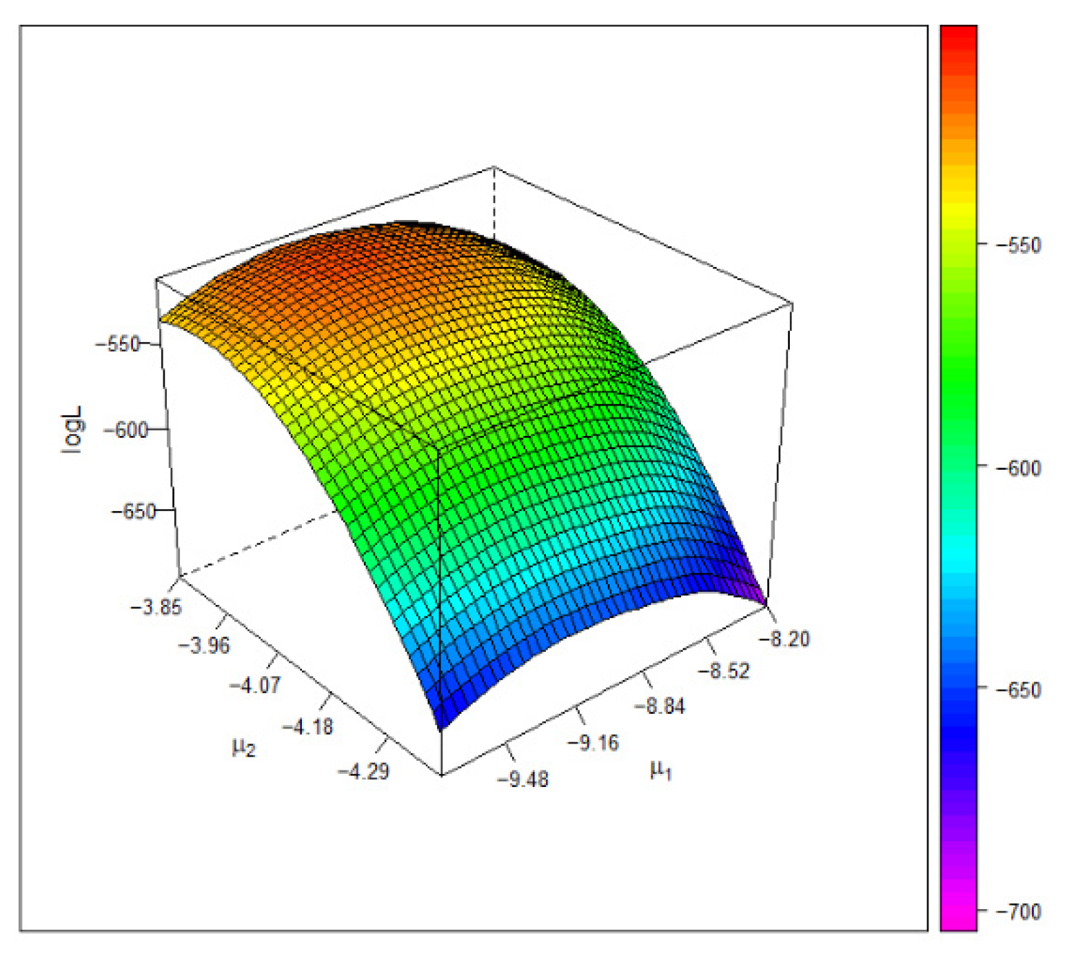
Figure 6 depicts the 3D plot of the log-likelihood surface under the Frank copula model. The plot shows that the estimate of the common mean ${\widehat{\mathit{\mu }}}_n^{\mathrm{Frank}}=\left(-9.20,-3.94\right)$ attains the global maximum of the log-likelihood function.

9. Extension to Non-Normal Models

So far, we have considered a common mean model under the marginal normality. This section explains how the proposed methods can be extended to non-normal models. For this reason, we specifically consider a common mean model under the marginal exponential distributions.

$${\stackrel{\_}{F}}_j\left(y\right)\equiv Pr(Y_{ij}>y)=\exp (-{\lambda }_{j}y), y>0, {\lambda }_j>0, j=1,2.$$

Thus, the common mean vector is $\mathit{\mu }=(1/{\lambda }_1,1/{\lambda }_2).$

We consider the Clayton copula to specify the bivariate distribution because it has simple derivatives with respect to the copula parameter [54]. Therefore, we propose a bivariate common mean Clayton copula model with exponential margins as follows:

$$Pr(Y_{i1}>y_1,Y_{i2}>y_2)=C_{{\alpha }_i}^{\mathrm{Clayton}}\left\{{\stackrel{\_}{F}}_1\left(y_1\right),{\stackrel{\_}{F}}_2\left(y_2\right)\right\}={\{\exp ({\alpha }_i{\lambda }_1{y}_1)+\exp ({\alpha }_i{\lambda }_2{y}_2)-1\}}^{-1/{\alpha }_i},$$

(4)

where ${\alpha }_i$ is known for $i=1,2,\dots ,n$. Note that copula $C_{{\alpha }_i}^{\mathrm{Clayton}}$ is a survival copula for ($Y_{i1},Y_{i2})$ as the usual way to model a survival function [22]. Using similar arguments to [55], the information matrix with respect to $\mathit{\lambda }=\left({\lambda }_1,{\lambda }_2\right)$ can be decomposed as

$$I_i\left(\mathit{\lambda }\right)=\left[\begin{array}{cc}\frac{1}{{\lambda }_1^2}& 0\\ 0& \frac{1}{{\lambda }_2^2}\end{array}\right]+\left[\begin{array}{cc}\frac{2{\alpha }_i^2\left({\alpha }_i+1\right)}{{\lambda }_1^2\left(3{\alpha }_i+1\right)}& -\frac{{\alpha }_i\left(2{\alpha }_i+1\right)}{{\lambda }_1{\lambda }_2}\varphi \left({\alpha }_i\right)\\ -\frac{{\alpha }_i\left(2{\alpha }_i+1\right)}{{\lambda }_1{\lambda }_2}\varphi \left({\alpha }_i\right)& \frac{2{\alpha }_i^2\left({\alpha }_i+1\right)}{{\lambda }_2^2\left(3{\alpha }_i+1\right)}\end{array}\right],$$

(5)

where

$$\varphi \left(\alpha \right)=\frac{1}{3\alpha +1}+\frac{1}{2\left(3\alpha +1\right)\left(2\alpha +1\right)}\left\{\Psi \left(\frac{1}{2\alpha }\right)-\Psi \left(\frac{\alpha +1}{2\alpha }\right)\right\}, \Psi \left(\alpha \right)=\frac{d^2\log \Gamma \left(\alpha \right)}{d{\alpha }^2}.$$

See Appendix A.3. for detailed derivations. The expression of $I_i\left(\mathit{\lambda }\right)$ is an extension of Theorem 3 to the exponential model. With the information matrix, the properties of the MLE and the asymptotic theory are similar to the normal models.

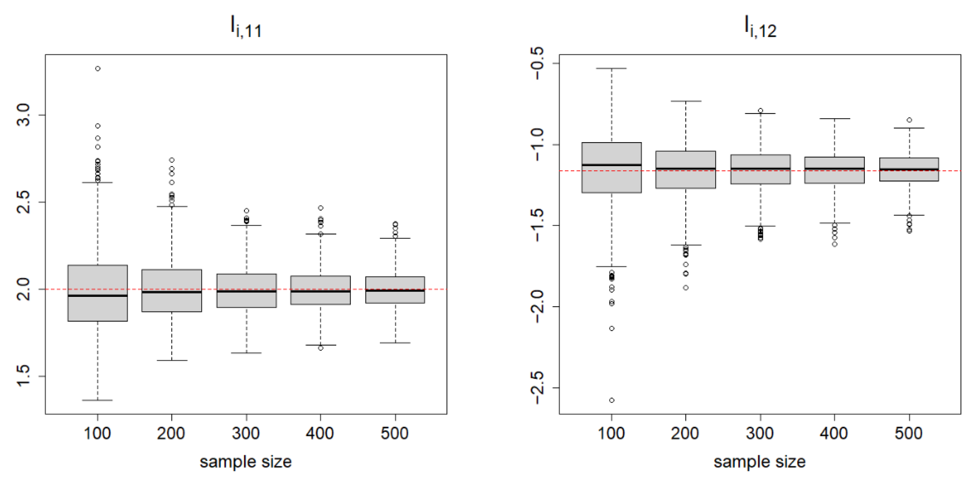
We conducted Monte Carlo simulations to examine the correctness of Equation (5) by comparing it with their empirical version. We set ${\lambda }_1={\lambda }_2=1$ and ${\alpha }_i=1$ for all $i$. We generated data $\left(Y_{i1},Y_{i2}\right), i=1,\dots ,n$ from the model in Equation (4) and computed the empirical versions of $I_{i,11}\left(\mathit{\lambda }\right)$ and $I_{i,12}\left(\mathit{\lambda }\right)$ as

$$\frac{1}{n}{\displaystyle \sum }_{i=1}^n\frac{{\partial }^2\log f_{i,\lambda }^{\mathrm{Clayton}}(Y_{i1},Y_{i2})}{\partial {\lambda }_1^2}, \frac{1}{n}{\displaystyle \sum }_{i=1}^n\frac{{\partial }^2\log f_{i,\lambda }^{\mathrm{Clayton}}(Y_{i1},Y_{i2})}{\partial {\lambda }_1\partial {\lambda }_2}.$$

The formulas for the derivatives of the log-density are found in Equations (A1) and (A2) in Appendix A.3. Our simulations were based on 1000 repetitions with $n\in \left\{100,200,300,400,500\right\}$.

Figure 7 depicts the simulation results based on 1000 repetitions. It clearly shows that the empirical versions are scattered around the theoretical values of $I_{i,11}\left(\mathit{\lambda }\right)=2$ and $I_{i,12}\left(\mathit{\lambda }\right)=-1.16$. The variability of the empirical versions vanishes as $n$ increases. The simulation results assert the correctness of Equation (5).

10. Conclusions

At present, copula models are very popular in all areas of science. Bivariate meta-analyses are among those research areas that require sophisticated copula-based methods and theories. Nonetheless, there are only a few studies on copula-based bivariate meta-analysis from a methodological/theoretical perspective. This article fully develops the methodologies and theories of the copula-based bivariate meta-analysis, specifically for estimating the common mean vector. These developments will provide solid methodological/theoretical bases that are not available to date.

In this article, we emphasize the flexibility of the proposed copula models that allow for a variety of dependence structures. In the two real data examples, we employed the log-likelihood value as a criterion for model selection (Section 8). Even if the best copula is selected, it still raises the issue of goodness-of-fit, which is difficult to assess under the meta-analysis setting. The classical methods, such as Kolmogorov–Smirnov or Cramér–von Mises type statistics, cannot be directly applied to the non-identically distributed samples for which the empirical distribution function is difficult to interpret. Therefore, the development of goodness-of-fit tests is a possible research direction.

The fundamental assumption made in the proposed model is the common mean model, with known within-study correlations. The common mean assumption, although convenient for summarizing the data for a small number of studies [56], may not always hold in real meta-analyses [6]. Therefore, the extension of the proposed estimator to random means (random-effects models) or ordered means [57,58] is an important direction for future research. To model the random effects, we need another bivariate copula. The estimation problem for these hierarchical copula-based models is beyond the scope of the paper. Nonetheless, the results presented in this paper serve as fundamental knowledge before the exploration of more advanced models.

References

- Gleser, L.J.; Olkin, L. Stochastically dependent effect sizes. In The Handbook of Research Synthesis; Russel Sage Foundation: New York, NY, USA, 1994. [Google Scholar]
- Riley, R.D. Multivariate meta-analysis: The effect of ignoring within-study correlation. J. R. Stat. Soc. Ser. A Stat. Soc. 2009, 172, 789–811. [Google Scholar] [CrossRef]
- Shih, J.-H.; Konno, Y.; Chang, Y.-T.; Emura, T. Estimation of a common mean vector in bivariate meta-analysis under the FGM copula. Statistics 2019, 53, 673–695. [Google Scholar] [CrossRef]
- Nissen, S.E.; Wolski, K. Effect of Rosiglitazone on the Risk of Myocardial Infarction and Death from Cardiovascular Causes. N. Engl. J. Med. 2007, 356, 2457–2471. [Google Scholar] [CrossRef] [PubMed] [Green Version]
- Yamaguchi, Y.; Maruo, K. Bivariate beta-binomial model using Gaussian copula for bivariate meta-analysis of two binary outcomes with low incidence. Jpn. J. Stat. Data Sci. 2019, 2, 347–373. [Google Scholar] [CrossRef] [Green Version]
- Mavridis, D.; Salanti, G. A practical introduction to multivariate meta-analysis. Stat. Methods Med. Res. 2011, 22, 133–158. [Google Scholar] [CrossRef]
- Copas, J.B.; Jackson, D.; White, I.; Riley, R.D. The role of secondary outcomes in multivariate meta-analysis. J. R. Stat. Soc. Ser. C Appl. Stat. 2018, 67, 1177–1205. [Google Scholar] [CrossRef]
- Burzykowski, T.; Molenberghs, G.; Buyse, M.; Geys, H.; Renard, D. Validation of surrogate end points in multiple randomized clinical trials with failure time end points. J. R. Stat. Soc. Ser. C Appl. Stat. 2001, 50, 405–422. [Google Scholar] [CrossRef] [Green Version]
- Rotolo, F.; Paoletti, X.; Michiels, S. surrosurv: An R package for the evaluation of failure time surrogate endpoints in individual patient data meta-analysis of randomized clinical trials. Comput. Methods Programs Biomed. 2018, 155, 189–198. [Google Scholar] [CrossRef]
- Rotolo, F.; Paoletti, X.; Burzykowski, T.; Buyse, M.; Michiels, S. A Poisson approach to the validation of failure time surrogate endpoints in individual patient data meta-analyses. Stat. Methods Med. Res. 2019, 28, 170–183. [Google Scholar] [CrossRef]
- Emura, T.; Sofeu, C.L.; Rondeau, V. Conditional copula models for correlated survival endpoints: Individual patient data meta-analysis of randomized controlled trials. Stat. Methods Med. Res. 2021, 30, 2634–2650. [Google Scholar] [CrossRef]
- Kuss, O.; Hoyer, A.; Solms, A. Meta-analysis for diagnostic accuracy studies: A new statistical model using beta-binomial dis-tributions and bivariate copulas. Stat. Med. 2014, 33, 17–30. [Google Scholar] [CrossRef]
- Nikoloulopoulos, A.K. A vine copula mixed effect model for trivariate meta-analysis of diagnostic test accuracy studies ac-counting for disease prevalence. Stat. Methods Med. Res. 2017, 26, 2270–2286. [Google Scholar] [CrossRef] [Green Version]
- Nikoloulopoulos, A.K. A D-vine copula mixed model for joint meta-analysis and comparison of diagnostic tests. Stat. Methods Med. Res. 2018, 28, 3286–3300. [Google Scholar] [CrossRef] [Green Version]
- Nikoloulopoulos, A.K. A multinomial quadrivariate D-vine copula mixed model for meta-analysis of diagnostic studies in the presence of non-evaluable subjects. Stat. Methods Med. Res. 2020, 29, 2988–3005. [Google Scholar] [CrossRef] [Green Version]
- Takeuchi, T.T. Constructing a bivariate distribution function with given marginals and correlation: Application to the galaxy luminosity function. Mon. Not. R. Astron. Soc. 2010, 406, 1830–1840. [Google Scholar] [CrossRef] [Green Version]
- Ota, S.; Kimura, M. Effective estimation algorithm for parameters of multivariate Farlie–Gumbel–Morgenstern copula. Jpn. J. Stat. Data Sci. 2021, 4, 1049–1078. [Google Scholar] [CrossRef]
- Ghosh, S.; Sheppard, L.W.; Holder, M.T.; Loecke, T.D.; Reid, P.C.; Bever, J.D.; Reuman, D.C. Copulas and their potential for ecology. Adv. Ecol. Res. 2020, 62, 409–468. [Google Scholar] [CrossRef]
- Alidoost, F.; Stein, A.; Su, Z. The use of bivariate copulas for bias correction of reanalysis air temperature data. PLoS ONE 2019, 14, e0216059. [Google Scholar] [CrossRef] [Green Version]
- Bhatti, M.I.; Do, H.Q. Recent development in copula and its applications to the energy, forestry and environmental sciences. Int. J. Hydrog. Energy 2019, 44, 19453–19473. [Google Scholar] [CrossRef]
- Emura, T.; Chen, Y.H. Analysis of Survival Data with Dependent Censoring: Copula-Based Approaches; JSS Research Series in Statistics; Springer: Singapore, 2018. [Google Scholar]
- Emura, T.; Matsui, S.; Rondeau, V. Survival Analysis with Correlated Endpoints, Joint Frailty-Copula Models; JSS Research Series in Statistics; Springer: Singapore, 2019. [Google Scholar]
- Emura, T.; Shih, J.-H.; Ha, I.D.; Wilke, R.A. Comparison of the marginal hazard model and the sub-distribution hazard model for competing risks under an assumed copula. Stat. Methods Med. Res. 2020, 29, 2307–2327. [Google Scholar] [CrossRef]
- Peng, M.; Xiang, L.; Wang, S. Semiparametric regression analysis of clustered survival data with semi-competing risks. Comput. Stat. Data Anal. 2018, 124, 53–70. [Google Scholar] [CrossRef]
- Huang, X.-W.; Wang, W.; Emura, T. A copula-based Markov chain model for serially dependent event times with a dependent terminal event. Jpn. J. Stat. Data Sci. 2020, 4, 917–951. [Google Scholar] [CrossRef]
- Shih, J.H. Common Mean. Copula: Bivariate Common Mean Vector under Copula Models; CRAN. 2022. Available online: https://CRAN.R-project.org/package=CommonMean.Copula (accessed on 8 January 2022).
- Berkey, C.S.; Hoaglin, D.C.; Antczak-bouckoms, A.; Mosteller, F.; Colditz, G.A. Meta-analysis of multiple outcomes by regression with random effect. Stat. Med. 1998, 17, 2537–2550. [Google Scholar] [CrossRef]
- Shinozaki, N. A note on estimating the common mean of k normal distributions and the stein problem. Commun. Stat.-Theory Methods 1978, 7, 1421–1432. [Google Scholar] [CrossRef]
- Malekzadeh, A.; Kharrati-Kopaei, M. Inferences on the common mean of several normal populations under hetero-scedasticity. Comput. Stat. 2018, 33, 1367–1384. [Google Scholar] [CrossRef]
- Gasparrini, A. Mvmeta: Multivariate and Univariate Meta-Analysis and Meta-Regression; CRAN. 2019. Available online: https://CRAN.R-project.org/package=mvmeta (accessed on 8 January 2022).
- Nelsen, R. An Introduction to Copulas. Technometrics. Lett. 2000, 42, 317. [Google Scholar] [CrossRef]
- Durante, F.; Sempi, C. Principles of Copula Theory; CRC/Chapman & Hall: Boca Raton, FL, USA, 2016. [Google Scholar]
- Morgenstern, D. Einfache Beispiele zweidimensionaler Verteilungen. Mitt. Für Math. Stat. 1956, 8, 34–235. [Google Scholar]
- Bairamov, I.G.; Kotz, S.; Bekci, M. New generalized Farlie-Gumbel-Morgenstern distributions and concomitants of order statistics. J. Appl. Stat. 2001, 28, 521–536. [Google Scholar] [CrossRef]
- Bairamov, I.; Kotz, S. Dependence structure and symmetry of Hunag-Kotz FGM distributions and their extensions. Metrika 2002, 56, 55–72. [Google Scholar] [CrossRef]
- Amini, M.; Jabbari, H.; Borzadaran, G.R.M. Aspects of Dependence in Generalized Farlie-Gumbel-Morgenstern Distributions. Commun. Stat.-Simul. Comput. 2011, 40, 1192–1205. [Google Scholar] [CrossRef]
- Domma, F.; Giordano, S. A copula-based approach to account for dependence in stress-strength models. Stat. Pap. 2012, 54, 807–826. [Google Scholar] [CrossRef]
- Chesneau, C. A new two-dimensional relation copula inspiring generalized version of the Farlie-Gumbel-Morgenstern copula. Res. Commun. Math. Math. Sci. 2021, 13, 99–128. [Google Scholar]
- Clayton, D.G. A model for association in bivariate life tables and its application in epidemiological studies of familial tendency in chronic disease incidence. Biometrika 1978, 65, 141–151. [Google Scholar] [CrossRef]
- Duchateau, L.; Janssen, P. The Frailty Model; Springer: New York, NY, USA, 2007. [Google Scholar]
- Gumbel, E.J. Distributions de valeurs extrêmes en plusieurs dimensions. Publ. Inst. Statist. Univ. Paris 1960, 9, 171–173. [Google Scholar]
- Frank, M.J. On the simultaneous associativity of F(x, y) and x+y−F(x, y). Aequ. Math. 1979, 19, 194–226. [Google Scholar] [CrossRef]
- Sklar, A. Fonctions de répartition à n dimensions et leurs marges. Publ. Inst. Statist. Univ. Paris 1959, 8, 229–231. [Google Scholar]
- Schucany, W.R.; Parr, W.C.; Boyer, J.E. Correlation structure in Farlie-Gumbel-Morgenstern distributions. Biometrika 1978, 65, 650–653. [Google Scholar] [CrossRef]
- Nelsen, R.B. Dependence and Order in Families of Archimedean Copulas. J. Multivar. Anal. 1997, 60, 111–122. [Google Scholar] [CrossRef] [Green Version]
- Bradley, R.A.; Gart, J.J. The asymptotic properties of ML estimators when sampling from associated populations. Biometrika 1962, 49, 205–214. [Google Scholar] [CrossRef]
- Emura, T.; Hu, Y.H.; Konno, Y. Asymptotic inference for maximum likelihood estimators under the special exponential family with double-truncation. Stat. Pap. 2017, 58, 877–909. [Google Scholar] [CrossRef]
- Shih, J.H. Copula-Based Statistical Inferences for a Common Mean Vector and Correlation Ratios Using Bivariate Data. Ph.D. Thesis, National Central University Library, Taoyuan, Taiwan, 2020. Available online: https://etd.lib.nctu.edu.tw/cgi-bin/gs32/ncugsweb.cgi/ccd=GLZeNP/record?r1=2&h1=2 (accessed on 3 October 2020).
- Shao, J. Mathematical Statistics; Springer: New York, NY, USA, 2003. [Google Scholar]
- Van der Vaart, A.W. Asymptotic Statistics; Cambridge University Press: Cambridge, UK, 1998. [Google Scholar]
- Lehmann, E.L.; Casella, G. Theory of Point Estimation, 2nd ed.; Springer: New York, NY, USA, 1998. [Google Scholar]
- Kontopantelis, E.; Reeves, D. Performance of statistical methods for meta-analysis when true study effects are non-normally distributed: A simulation study. Stat. Methods Med Res. 2010, 21, 409–426. [Google Scholar] [CrossRef]
- Jackson, D.; White, I.R.; Riley, R.D. A matrix-based method of moments for fitting the multivariate random effects model for meta-analysis and meta-regression. Biom. J. 2013, 55, 231–245. [Google Scholar] [CrossRef] [Green Version]
- Schepsmeier, U.; Stöber, J. Derivatives and Fisher information of bivariate copulas. Stat. Pap. 2013, 55, 525–542. [Google Scholar] [CrossRef]
- Oakes, D. A Model for Association in Bivariate Survival Data. J. R. Stat. Soc. Ser. B Stat. Methodol. 1982, 44, 414–422. [Google Scholar] [CrossRef]
- Nakatochi, M.; Kanai, M.; Nakayama, A.; Hishida, A.; Kawamura, Y.; Ichihara, S.; Matsuo, H. Genome-wide me-ta-analysis identifies multiple novel loci associated with serum uric acid levels in Japanese individuals. Commun. Biol. 2019, 2, 1–10. [Google Scholar] [CrossRef]
- Taketomi, N.; Konno, Y.; Chang, Y.-T.; Emura, T. A Meta-Analysis for Simultaneously Estimating Individual Means with Shrinkage, Isotonic Regression and Pretests. Axioms 2021, 10, 267. [Google Scholar] [CrossRef]
- Taketomi, N.; Michimae, H.; Chang, Y.-T.; Emura, T. meta.shrinkage: An R package for meta-analyses for simultaneously estimating individual means. Algorithms, 2022; accepted. [Google Scholar]
Figure 1.
The boundary correction for the correlation coefficient under the bivariate FGM and Clayton models. The first step forces the correlation to fall in a range that can be modeled by the chosen copula. The second step transforms the corrected correlation to the corresponding copula parameter.
Figure 2.
The boxplots summarizing the 1000 repetitions for with true parameter under the copula parameters , , or . The sample size varies from to .
Figure 3.
The MLE and the 95% CE (colored region) for the common means based on the exam score data. The copulas are signified by colors: blue = FGM; gray = Clayton; orange = Gumbel; pink = Frank; green = normal.
Figure 4.
The 3D plot of the log-likelihood value under the Gumbel copula based on the entrance exam data. The maximum occurs at .
Figure 5.
The MLE and the 95% CE (colored region) for the common means based on the blood pressure data. The correspondence copulas of the colored regions are: blue = FGM; gray = Clayton; orange = Gumbel; pink = Frank; green = normal.
Figure 6.
The 3D plot of the log-likelihood value under the Frank copula based on the blood pressure data. The maximum occurs at .
Figure 7.
The boxplots summarizing the 1000 repetitions for the empirical versions of and (dashed lines) under the Clayton copula model in Equation (4) with parameter = 1. The sample size varies from to .