Virtual Attractive-Repulsive Potentials Control Theory: A Review and an Extension to Riemannian Manifolds

Abstract

The present paper is concerned with an instance of automatic control for autonomous vehicles based on the theory of virtual attractive-repulsive potentials (VARP). The first part of this paper presents a review of the VARP control theory as developed specifically by B. Nguyen, Y.-L. Chuang, D. Tung, C. Hsieh, Z. Jin, L. Shi, D. Marthaler, A. Bertozzi and R. Murray, in the paper ‘Virtual attractive-repulsive potentials for cooperative control of second order dynamic vehicles on the Caltech MVWT’, which appeared in the Proceedings of the 2005 American Control Conference, (Portland, OR, USA) held in June 2005 (pp. 1084–1089). The aim of the first part of the present paper is to recall the mathematical and logical steps that lead to controlling an autonomous robot by a VARP-based control theory. The concepts recalled in the first part of the present paper, with special reference to the physical interpretation of the terms in the developed control field, serve as the starting point to develop a more convoluted control theory for (second-order) dynamical systems whose state spaces are (possibly high-dimensional) curved manifolds. The second part of this paper is, in fact, devoted to extending the classical VARP control theory to regulate dynamical systems whose state spaces possess the mathematical structure of smooth manifolds through manifold calculus. Manifold-type state spaces present a high degree of symmetry, due to mutual non-linear constraints between single physical variables. A comprehensive set of numerical experiments complements the review of the VARP theory and the theoretical developments towards its extension to smooth manifolds.

1. Introduction

Most control problems of interest in engineering and applied sciences concern positioning, path planning and obstacles avoidance. A noteworthy example is given by the need of commanding a spacecraft in such a way that it avoids bright objects yet maintaining communication with ground station, as discussed in [1]. Further noteworthy examples are found in landing maneuvering of manned electric vehicles [2], interception of mobile search vehicles [3], and manual guidance of robotic manipulators [4]. Virtual potentials prove effective in solving non-linear control problems as they appear to be versatile and widely applicable. In order to control a particular dynamical system, it is necessary to build a virtual potential field. Such construction may be effected within a number of mathematical frameworks. For instance, a virtual potential field may be constructed by the use of harmonic functions and Laplace’s equations [5,6], artificial gyroscopic forces [7] and stream functions from fluid dynamics [8].

The study of potential fields took originally its moves from physics, chemistry and biology [9] although its versatility makes it advantageous in several different fields such as vehicle coordination [10]. In fact, potential fields have been widely used to control different types of vehicles such as cylindrical robots [11], helicopters [12], road vehicles [13] and unmanned ground vehicles [14].

A special acknowledgment should be paid to Koditschek and Rimon who, in a series of papers, laid the foundation of the VARP theory. In particular, in the contribution [15], the authors proposed “a methodology for exact robot motion planning and control that unifies the purely kinematic path planning problem with the lower level feedback controller design”. The innovative aspect of their work was to encode complete information about a freespace and goal in the form of a special virtual potential function, termed navigation function. Such navigation function gives rise to a feedback controller for the robot that guarantees collision-free motion and convergence to the destination. The authors of [15] developed a family of navigation functions that serve to guide a point-mass robot through a generalized sphere world. The simplest member of such family of navigation functions is obtained by puncturing a disk by an arbitrary number of smaller disjoint disks that represent obstacles. More complex spaces (and obstacles) are obtained from this model by suitable coordinate transformations. The study [15] was essentially devoted to planar scenarios and appears as an application of more general results presented earlier in [16], where the general problem of constructing navigation functions on arbitrary manifolds (not only those obtainable as deformations of sphere words) was dealt with.

Over the years, potential fields have been applied to constrained attitude control, as they enable to handle simultaneously a large number of forbidden and mandatory zones, while guaranteeing computational tractability and convergence [17]. Potential fields have also been applied to slew maneuver of satellites; see, e.g., the paper [18] that introduced a ‘Sun avoidance potential’. The manuscript [19] introduced the notion of exponential repulsive potential whose gradient returns a protection control field to prevent aircraft accidents. The contribution [20] utilizes virtual potential functions to generate trajectories to be used as initial guesses for a ‘general pseudospectral optimal control’ algorithm. The research work published in [21] presents a real-time hybrid guidance method which fuses the flexibility and robustness of harmonic potential functions with a rapidly-expanding random-tree method; such research outcome allows to plan near-fuel-optimal trajectories on cluttered environments. The paper [22] outlines a method based on the theory of virtual potential fields combined with sliding mode control for spacecraft maneuvers in the presence of obstacles; guidance and control algorithms devised in such manner were validated through a six degree-of-freedom omorbital simulator. Guidance algorithms based on artificial potential functions play an increasingly important role in hazard avoidance, although local minima might cause a spacecraft to be unable to reach the desired target landing point in complex terrains. In the paper [23], a novel hazard avoidance guidance method was developed by improving the traditional virtual potential function structure.

Potential fields may also be utilized in conjunction with other control strategies. For example, Cao et al. [24] suggested using potential fields in order to adjust the path planned by a neural network in such a way that an autonomous underwater vehicle avoids obstacles. Baxter et al. [25] developed a control method based on the exchange of information regarding potential fields between robots belonging to the same local group of vehicles. Huang [26] proposed a path and speed planning strategy based on the use of a potential field for a robot located in a dynamic environment where obstacles and targets are moving.

Potential function-based proportional-derivative as well as augmented-proportional-derivative control laws were developed in [27] to govern the motion of an underactuated autonomous underwater vehicle in an obstacle-rich environment; for obstacle avoidance, a mathematical potential function was devised, which formulates the repulsive force between the vehicle and the solid obstacles intersecting a vehicle’s desired path. The guidance and control framework proposed in [28] integrates offline optimal path planning with a safety distance constrained A* algorithm, and an online extended adaptively-weighted virtual potential field-based path following approach with dynamic collision avoidance, based on unmanned surface vehicles maneuvering response times. An adaptive potential function approach originally developed for ground robots was modified in [29] and employed as a guidance law for a class of rotary-wing unmanned aerial vehicles that must also avoid obstacles located in a three-dimensional workspace.

The use of potential fields has been extensively studied and some alternatives have been proposed to overcome those difficulties that it might entail. An often encountered difficulty is that a local minimum in the potential field might trap a controlled vehicle and consequently prevent it from reaching the global minimum, which represents the actual goal. Lee et al. [30] proposed a solution to such problem based on the placement of a virtual repulsive obstacle in a local minimum to keep a robot adequately distant from it. A further solution to the aforementioned problem is to invoke hybrid strategies based on virtual potentials and BUG algorithms [31,32,33,34,35], as proposed by Wang et al. [36]. A further common difficulty to be aware of in the use of potential fields is the oscillation of the controlled vehicle around obstacles and targets. Several proposals have been presented to address such problem. Ren et al. [37] proposed the use of a modified Newton’s method (MNM) for robot navigation based on an approximation of a potential field function, which is often a complicated non-linear function, by a quadratic form. Li et al. [38] presented a regression search method, based on an improved artificial potential field, capable of mitigating local minima as well as oscillations. Such solution consists in redefining potential functions in order to delete local minima and in utilizing virtual local targets for a robot to escape oscillations. Regression search was then used to optimize the path followed by a vehicle.

On the basis of the consistent literature accumulated on this subject, the authors of [39] proposed a workable feedback control theory, termed VARP (that stands for virtual attractive-repulsive potentials) that they applied to drive a simple robotic platform (named ‘Kelly robot’). The control algorithm developed by the authors Nguyen, Chuang, Tung, Hsieh, Jin, Shi, Marthaler, Bertozzi and Murray was proven effective through experiments conducted at the Caltech University’s multi-vehicle wireless testbed facility. One of the main ideas developed in the paper [39] was to endow each element in the environment, including the controlled robot as well as obstacles and targets, by both an attractive and a repulsive potential to improve maneuverability and control flexibility.

Since such VARP control theory was specifically designed to control a simple robotic platform with three degrees of freedom (two positional coordinates and an orientation angle), it cannot be extended directly to more complicated dynamical systems such as a six degree-of-freedom drone. The aim of the present paper is to design an artificial control field based on the virtual attractive-repulsive potentials to be applied to a wide class of dynamical systems. In fact, in the present paper, a VARP-based method will be developed to control different dynamical systems whose state-space equations insist on different mathematical spaces. In particular, manifold-type state spaces shall be dealt with, which present a high degree of symmetry, due to mutual non-linear constraints that single physical descriptive variables are subjected to. In order to formulate a VARP-on-manifold control theory, a special branch of mathematics will be accessed, namely manifold calculus. In addition, in order to implement the devised VARP-on-manifold control theory on a computing platform, specific numerical algorithms have been developed, which are based on manifold calculus. As a reference on coordinate-free (embedded) manifold calculus in system theory and control, interested readers might consult the tutorial paper [40].

The present document is organized as follows.

Section 2 describes the theory of virtual attractive-repulsive potentials as introduced in [9,39]. The aim of this section is to recall the main concepts related to the VARP theory and its main theoretical features.

Section 3 presents a description of a prototypical wheeled robot, used at the Caltech University for testing the devised VARP principle. This section also explains how to implement the VARP control method on a computation platform in order to evaluate numerically its effectiveness in controlling a small robot. In particular, in this section, results of numerical experiments obtained by varying the parameters of the VARP method will be presented and discussed, in order to illustrate its features. The numerical experiments were performed on purpose by a low-precision numerical scheme (the forward Euler method) to recap this method that will be extended to manifold in the following section. The analysis presented in this section is propaedeutic to the following development as the understanding of details concerning the application of the VARP control theory to drive a small robot will be beneficial in extending the VARP theory to control more complicated systems whose state evolves on smooth manifolds.

Section 4 recalls generalities of Riemannian manifolds and recaps the theory of second-order dynamical system whose state equations are formulated on the tangent bundle of a manifold. This section then illustrates how the VARP method can be extended in order to control a dynamical system whose state equations are formulated on a Riemannian manifold (M-VARP). As a case-study, the M-VARP method will be illustrated on the manifold ${\mathbb{S}}^2$ (a three-dimensional unit sphere). The numerical algorithms to implement such control scheme will be shown to arise from a specifically-tailored version of a forward Euler method on manifolds.

Section 5 completes the present document, focusing on conclusions and future works.

2. Introduction to the VARP Control Theory

The virtual attractive-repulsive potentials-based control theory stems from the construction of a virtual potential field made of virtual points. To each point it will be assigned both an attractive and a repulsive potential. The points on the virtual field may represent obstacles, targets or different sorts of objects in a state space. In this document, we shall recall how the VARP control theory may be employed to control different dynamical systems associated to different state spaces.

2.1. Virtual Potentials for Swarming Models in Biology

Virtual potentials provide a convenient framework for autonomous vehicle control and path planning. Such potentials arise from swarming models in biology and may be formulated as in the discrete particle model proposed by the Levine-Rappel-Cohen group [9].

Given N particles labeled $i=1,2,\dots ,N$, the model proposed in [9] that governs the motion of each particle is described by:

$$\begin{array}{c}\hfill \left\{\begin{array}{c}{m}_i\frac{\mathrm{d}{\overrightarrow{v}}_i}{\mathrm{d}t}=\alpha {\widehat{f}}_i-\beta {\overrightarrow{v}}_i-\overrightarrow{\mathrm{grad}}V,\hfill \\ \frac{\mathrm{d}{\overrightarrow{x}}_i}{\mathrm{d}t}={\overrightarrow{v}}_i,\hfill \end{array}\right.\end{array}$$

(1)

where $m_i>0$ denotes the mass of each particle, ${\overrightarrow{x}}_i\in {\mathbb{R}}^3$ and ${\overrightarrow{v}}_i\in {\mathbb{R}}^3$ its position and velocity, respectively. Each particle experiences a unit-norm self-propelling force ${\widehat{f}}_i\in {\mathbb{R}}^3$ with fixed magnitude $\alpha >0$. To prevent the particles from reaching large speeds, a friction force with coefficient $\beta >0$ was introduced.

In addition, each particle is subjected to an attraction force (that depends only on the distance from one particle to the others) which is characterized by an interaction range ${\ell }_a>0$. This force is responsible for the aggregation of the particles. To prevent a collapse of the aggregate, a shorter-range repulsive force was introduced with interaction range ${\ell }_r>0$. The authors of [9] verified experimentally that qualitative results are independent of the explicit expression of the interaction potential. Levine’s model is, in fact, based on exponentially decaying interactions described by virtual potentials of the kind:

$$V:=-\sum _{j,j\ne i}{C}_{\mathrm{a}}exp\left(-\frac{∥{\overrightarrow{x}}_i-{\overrightarrow{x}}_j∥}{{\ell }_{\mathrm{a}}}\right)+\sum _{j,j\ne i}{C}_{\mathrm{r}}exp\left(-\frac{∥{\overrightarrow{x}}_i-{\overrightarrow{x}}_j∥}{{\ell }_{\mathrm{r}}}\right),$$

(2)

where $C_{\mathrm{a}}>0$, $C_{\mathrm{r}}>0$ determine the strength of the attractive and repulsive forces, respectively. (The original potential has reversed sign with respect to the one reported here: We have chosen the above form for consistency with the remainder of the paper.) We underline that Levine’s model is based on parameters whose values are identical for each particle, while in the next sections we shall define specific parameters for each obstacle and target.

2.2. VARP Control Theory

From Levine’s model, a VARP theory to control and coordinate a group of vehicles was developed in [39]. Given an i-th vehicle and N concurrent agents labeled $j=1,2,\dots ,N$, the VARP control method is described by the following general coupled equations:

$$\left\{\begin{array}{c}\frac{\mathrm{d}{\overrightarrow{z}}_i}{\mathrm{d}t}={\overrightarrow{w}}_i,\hfill \\ m_i\frac{\mathrm{d}{\overrightarrow{w}}_i}{\mathrm{d}t}=\alpha {\widehat{\xi }}_i-\beta {\overrightarrow{w}}_i-{\overrightarrow{\mathrm{grad}}}_{{\overrightarrow{z}}_i}{\displaystyle \sum _{\begin{array}{c}j=1\\ j\ne i\end{array}}^N}\left[V_j^{\mathrm{r}}\left(d({\overrightarrow{z}}_i,{\overrightarrow{q}}_j)\right)-V_j^{\mathrm{a}}\left(d({\overrightarrow{z}}_i,{\overrightarrow{q}}_j)\right)\right],\hfill \end{array}\right.$$

(3)

where the notation used has the following meaning:

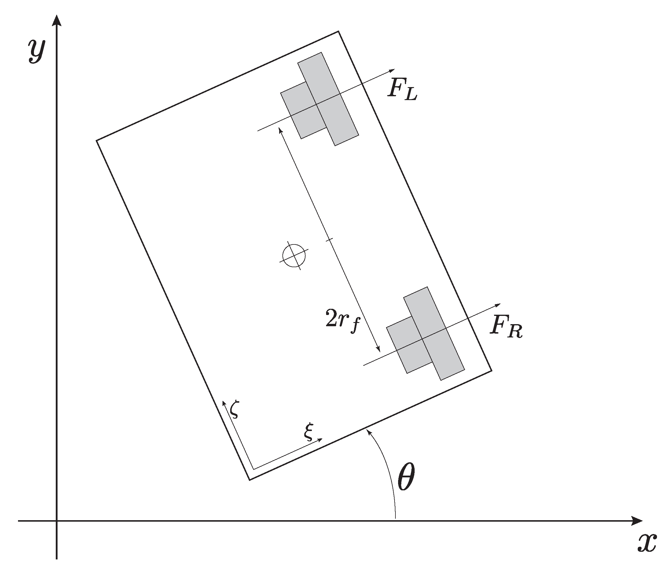
• the symbol ${\widehat{\xi }}_i$ denotes a unit vector in a reference frame attached to each i-th vehicle rotated with respect to the inertial reference frame $\widehat{x}-\widehat{y}$ by an angle $\theta$, as illustrated in Figure 1;
• the symbol ${\overrightarrow{z}}_i=(z_{x_i},z_{y_i})$ denotes the position of the i-th vehicle at time t;
• the symbol ${\overrightarrow{w}}_i$ denotes the velocity of the i-th vehicle at time t;
• the constant $m_i$ denotes the mass of the i-th vehicle;
• the quantity $d({\overrightarrow{z}}_i,{\overrightarrow{q}}_j)=\parallel {\overrightarrow{z}}_i-{\overrightarrow{q}}_j\parallel$ denotes the Euclidean distance between the i-th vehicle and the j-th agent that is located at ${\overrightarrow{q}}_j=(q_{x_j},q_{y_j})$ at time t; in this context, an agent could represent an obstacle, a target point or another vehicle; in the case of multiple vehicle control, each vehicle other than the i-th one will be considered as an obstacle for the i-th vehicle, therefore the position of the i-th vehicle is denoted as ${\overrightarrow{z}}_i$ while the position of the j-th obstacle will be denoted as ${\overrightarrow{q}}_j$;
• the constant $\alpha >0$ denotes the magnitude of the self-propelling force; the self-propelling term determines a speed-up of the motion of a vehicle and helps escaping unwanted plateaus of the potential function; the amplitude $\alpha$ of the self-propelling term modulates these positive effects but may also cause instability in the system and unwanted oscillations around the way-point;
• the constant $\beta >0$ denotes a friction coefficient; viscous-type friction brakes the motion of a vehicle and generally has the positive effect of stabilizing its motion; friction has however the side effect of slowing down the navigation of a vehicle; the friction coefficient $\beta$ should hence be chosen sufficiently large to stabilize the system and sufficiently small not to delay excessively reaching the way-point;
• symbols $V_j^{\mathrm{a}}$ e $V_j^{\mathrm{r}}$ denote, respectively, the attractive and repulsive potential functions, defined as:

  $$V_j^{\mathrm{a}}\left(\varphi \right):=C_j^{\mathrm{a}}{e}^{-\varphi /{\ell }_j^{\mathrm{a}}},V_j^{\mathrm{r}}\left(\varphi \right):=C_j^{\mathrm{r}}{e}^{-\varphi /{\ell }_j^{\mathrm{r}}},$$

  (4)

  where constants $C_j^{\mathrm{a}}>0$, $C_j^{\mathrm{r}}>0$ denote the “magnitude of the potentials”, constants ${\ell }_j^{\mathrm{a}}>0$, ${\ell }_j^{\mathrm{r}}>0$ their “characteristic lengths”, and $\varphi$ denotes a real positive variable.

In the biology-inspired model proposed in [9], potentials serve to organize a group of self-propelled particles into a mill-like formation. In the VARP theory, attractive potentials are used to direct vehicles towards way points and attractive/repulsive potentials to keep vehicles avoiding each other and stationary obstacles. Namely, a point-to-point control strategy arises from the VARP theory.

3. VARP Control Theory Applied to a Wheeled Robot Navigation on a Plane

In the present section, we shall recall how the VARP control theory was exploited to control a small self-driven wheeled vehicle termed ‘Kelly robot’. Full mathematical details are reported and commented, since these details are deemed interesting to understand the meaning of each terms in Equation (3) in view of a successive extension of the plain VARP theory to Riemannian manifolds.

3.1. Kelly Robot Description and Mathematical Model

The Kelly robot was developed at the Caltech University and it was taken as a prototypical model for testing the VARP feedback control principle. Such robot was realized as a fiberglass structure that includes an onboard micro-controller (that implements the algorithm for movement control), onboard sensors and a 802.11b wireless card through which it may communicate. Further interesting characteristics are low-friction omnidirectional casters (which allow the Kelly robot to move over the floor) and two high-performance ducted fans, each capable of producing up to $4.5$ N of continuous thrust. Caltech tests have been conducted at the Multi-Vehicle Wireless Testbed (MVWT), which is a platform designed for validating theoretical advances in multiple-vehicle coordination and cooperative control. The MVWT is equipped by a wireless network, an arena for multi-vehicle operations, a lab positioning system based on overhead cameras, and a computer network. The smooth floor where the vehicles maneuver has dimensions of approximately 6.5 m × 7.0 m. Vehicles are marked with binary symbols on their hats, that the vision system uses to identify their location and orientation.

The Kelly robot is modeled by a nonlinear dynamical system described by the following equations:

$$\begin{array}{c}\hfill \left\{\begin{array}{cc}m\frac{\mathrm{d}u}{\mathrm{d}t}\hfill & =-\mu u+(F_R+F_L)cos\theta ,\hfill \\ m\frac{\mathrm{d}v}{\mathrm{d}t}\hfill & =-\mu v+(F_R+F_L)sin\theta ,\hfill \\ J\frac{\mathrm{d}\Omega }{\mathrm{d}t}\hfill & =-\psi \Omega +(F_R-F_L)r_f,\hfill \end{array}\right.\end{array}$$

(5)

where the symbols used take the following meanings:

• the symbols $F_R$ and $F_L$ denote the magnitudes of the forces generated by, respectively, the ducted fans located at the right-hand side and the left-hand side of the robot’s rear end, which are separated by a distance $2r_f$ as shown in Figure 1, where $r_f=0.124$ m;
• the constant m denotes the mass of the Kelly vehicle, whose value is $5.15$ kg;
• the constant $\mu$ denotes the linear friction coefficient, whose value, in the case of the MVWT testbed, is $4.5$ kg/s;
• the constant $\psi$ denotes an angular friction coefficient, whose value, in the case of the MVWT testbed, is $0.064$ kg m${}^2$/s;
• the variables $u=\frac{\mathrm{d}{z}_x}{\mathrm{d}t}$ and $v=\frac{\mathrm{d}{z}_y}{\mathrm{d}t}$ denote the components of the linear velocity of the vehicle, where $z_x$ and $z_y$ denote the positional coordinates of the vehicle;
• the variable $\Omega =\frac{\mathrm{d}\theta }{\mathrm{d}t}$ denotes the angular velocity with respect to the $\widehat{x}-\widehat{y}$ reference frame, expressed in rad/s, and the angle $\theta$ denotes the orientation of the vehicle (with respect to the same $\widehat{x}-\widehat{y}$ reference frame), expressed in radians;
• the constant J denotes the moment of inertia of the vehicle and its value is $0.5$ kg m${}^2$.

The quantities $\mu$, $\psi$, m, J and $r_f$ denote physical constants of the vehicle, while the variables u, v, $\Omega$ and $\theta$ are the results of its dynamics and play the role of internal states of a vehicle’s model. The quantities $F_R$ and $F_L$ may be regarded as inputs of the system and are subjected to the action of a controlling algorithm, which may determine their amplitude according to a desired control strategy.

The aim of the VARP-based design is to determine expressions of the forces $F_R$ and $F_L$ in such a way that the mathematical model encoded by Equation (5) transforms into the VARP Equation (3). Such development is detailed in the next section.

3.2. VARP Control Theory Applied to the Kelly Robot

Combining Kelly robot’s equations of motion (5) and the equations that describe the VARP theory (3), it is possible to obtain a direct definition of the right-hand and left-hand fan forces, which represent input/control variables in the mathematical model (5).

Plugging into the second equation of (3) the explicit expressions of the potential functions leads to:

$$\begin{array}{c}\hfill {\overrightarrow{f}}_i:=\alpha \widehat{{\xi }_i}-\beta {\overrightarrow{w}}_i-{\overrightarrow{\mathrm{grad}}}_{{\overrightarrow{z}}_i}\sum _{\begin{array}{c}j=1\\ j\ne i\end{array}}^N\left[-C_j^{\mathrm{a}}{e}^{-\frac{d({\overrightarrow{z}}_i,{\overrightarrow{q}}_j)}{{\ell }_j^{\mathrm{a}}}}+C_j^{\mathrm{r}}{e}^{-\frac{d({\overrightarrow{z}}_i,{\overrightarrow{q}}_j)}{{\ell }_j^{\mathrm{r}}}}\right].\end{array}$$

(6)

Applying the gradient to the sum we obtain:

$$\begin{array}{c}\hfill \begin{array}{cc}\hfill {\overrightarrow{f}}_i& =\alpha {\widehat{\xi }}_i-\beta {\overrightarrow{w}}_i-\sum _{\begin{array}{c}j=1\\ j\ne i\end{array}}^N\left[\left(\frac{C_j^{\mathrm{a}}}{{\ell }_j^{\mathrm{a}}}{e}^{-\frac{d({\overrightarrow{z}}_i,{\overrightarrow{q}}_j)}{{\ell }_j^{\mathrm{a}}}}-\frac{C_j^{\mathrm{r}}}{{\ell }_j^{\mathrm{r}}}{e}^{-\frac{d({\overrightarrow{z}}_i,{\overrightarrow{q}}_j)}{{\ell }_j^{\mathrm{r}}}}\right)\frac{(z_{x_i}-q_{x_j})\widehat{x}+(z_{y_i}-q_{y_j})\widehat{y}}{d({\overrightarrow{z}}_i,{\overrightarrow{q}}_j)}\right].\hfill \end{array}\end{array}$$

(7)

The vehicle-fixed $\widehat{\xi }-\widehat{\zeta }$ reference frame is obtained by rotating the inertial $\widehat{x}-\widehat{y}$ reference frame by an angle $\theta$. Namely, the two reference frames are related by:

$$\begin{array}{c}\hfill \left\{\begin{array}{c}\widehat{x}=\widehat{{\xi }_i}cos{\theta }_i-\widehat{{\zeta }_i}sin{\theta }_i,\hfill \\ \widehat{y}=\widehat{{\xi }_i}sin{\theta }_i+\widehat{{\zeta }_i}cos{\theta }_i.\hfill \end{array}\right.\end{array}$$

(8)

Plugging Equation (8) in Equation (7) gives:

$$\begin{array}{c}\hfill \begin{array}{cc}\hfill {\overrightarrow{f}}_i& =\alpha {\widehat{\xi }}_i-\beta {\overrightarrow{w}}_i+\hfill \\ \hfill & -\sum _{\begin{array}{c}j=1\\ j\ne i\end{array}}^N[\left(\frac{C_j^{\mathrm{a}}}{{\ell }_j^{\mathrm{a}}}{e}^{-\frac{d({\overrightarrow{z}}_i,{\overrightarrow{q}}_j)}{{\ell }_j^{\mathrm{a}}}}-\frac{C_j^{\mathrm{r}}}{{\ell }_j^{\mathrm{r}}}{e}^{-\frac{d({\overrightarrow{z}}_i,{\overrightarrow{q}}_j)}{{\ell }_j^{\mathrm{r}}}}\right)\frac{(z_{x_i}-q_{x_j})cos{\theta }_i+(z_{y_i}-q_{y_j})sin{\theta }_i}{d({\overrightarrow{z}}_i,{\overrightarrow{q}}_j)}{\widehat{\xi }}_i+\hfill \\ \hfill & +\left(\frac{C_j^{\mathrm{a}}}{C_j^{\mathrm{a}}}{e}^{-\frac{d({\overrightarrow{z}}_i,{\overrightarrow{q}}_j)}{C_j^{\mathrm{a}}}}-\frac{C_j^{\mathrm{r}}}{{\ell }_j^{\mathrm{r}}}{e}^{-\frac{d({\overrightarrow{z}}_i,{\overrightarrow{q}}_j)}{C_j^{\mathrm{r}}}}\right)\frac{-(z_{x_i}-q_{x_j})sin{\theta }_i+(z_{y_i}-q_{y_j})cos{\theta }_i}{d({\overrightarrow{z}}_i,{\overrightarrow{q}}_j)}{\widehat{\zeta }}_i].\hfill \end{array}\end{array}$$

(9)

The forcing term (9) may be decomposed in components along the ${\widehat{\xi }}_i$ and ${\widehat{\zeta }}_i$ axes. From the scalar product between both sides of the relation (9) and the unit vector $\widehat{{\xi }_i}$ we obtain, in particular, the component of the forcing term ${\overrightarrow{f}}_i$ along the direction of motion:

$$\begin{array}{c}\hfill \begin{array}{cc}\hfill {\overrightarrow{f}}_i^{\Vert }& :=\alpha {\widehat{\xi }}_i-\beta {\overrightarrow{w}}_i+\hfill \\ \hfill & -\sum _{\begin{array}{c}j=1\\ j\ne i\end{array}}^N\left[\left(\frac{C_j^{\mathrm{a}}}{{\ell }_j^{\mathrm{a}}}{e}^{-\frac{d({\overrightarrow{z}}_i,{\overrightarrow{q}}_j)}{{\ell }_j^{\mathrm{a}}}}-\frac{C_j^{\mathrm{r}}}{{\ell }_j^{\mathrm{r}}}{e}^{-\frac{d({\overrightarrow{z}}_i,{\overrightarrow{q}}_j)}{{\ell }_j^{\mathrm{r}}}}\right)\frac{(z_{x_i}-q_{x_j})cos{\theta }_i+(z_{y_i}-q_{y_j})sin{\theta }_i}{d({\overrightarrow{z}}_i,{\overrightarrow{q}}_j)}\right]{\widehat{\xi }}_i.\hfill \end{array}\end{array}$$

(10)

The component of the force along the ${\widehat{\xi }}_i$ direction, in turn, may be decomposed in two components, one along the $\widehat{x}$ direction, and one along the $\widehat{y}$ direction, which read, respectively:

$$\begin{array}{c}\hfill \begin{array}{cc}\hfill f_{i,x}^{\Vert }& :=\alpha cos{\theta }_i-\beta u_i+\hfill \\ \hfill & -\sum _{\begin{array}{c}j=1\\ j\ne i\end{array}}^N\left[\left(\frac{C_j^{\mathrm{a}}}{{\ell }_j^{\mathrm{a}}}{e}^{-\frac{d({\overrightarrow{z}}_i,{\overrightarrow{q}}_j)}{{\ell }_j^{\mathrm{a}}}}-\frac{C_j^{\mathrm{r}}}{{\ell }_j^{\mathrm{r}}}{e}^{-\frac{d({\overrightarrow{z}}_i,{\overrightarrow{q}}_j)}{{\ell }_j^{\mathrm{r}}}}\right)\frac{(z_{x_i}-q_{x_j}){cos}^2{\theta }_i+(z_{y_i}-q_{y_j})cos{\theta }_{i}sin{\theta }_i}{d({\overrightarrow{z}}_i,{\overrightarrow{q}}_j)}\right],\hfill \end{array}\end{array}$$

(11)

$$\begin{array}{c}\hfill \begin{array}{cc}\hfill f_{i,y}^{\Vert }& :=\alpha sin{\theta }_i-\beta v_i+\hfill \\ \hfill & -\sum _{\begin{array}{c}j=1\\ j\ne i\end{array}}^N\left[\left(\frac{C_j^{\mathrm{a}}}{{\ell }_j^{\mathrm{a}}}{e}^{-\frac{d({\overrightarrow{z}}_i,{\overrightarrow{q}}_j)}{{\ell }_j^{\mathrm{a}}}}-\frac{C_j^{\mathrm{r}}}{{\ell }_j^{\mathrm{r}}}{e}^{-\frac{d({\overrightarrow{z}}_i,{\overrightarrow{q}}_j)}{{\ell }_j^{\mathrm{r}}}}\right)\frac{(z_{x_i}-q_{x_j})cos{\theta }_{i}sin{\theta }_i+(z_{y_i}-q_{y_j}){sin}^2{\theta }_i}{d({\overrightarrow{z}}_i,{\overrightarrow{q}}_j)}\right].\hfill \end{array}\end{array}$$

(12)

In addition, from the scalar product between the force (9) and the unit vector $\widehat{{\zeta }_i}$, we obtain the component of the total forcing term perpendicular to the direction of motion, which reads:

$$\begin{array}{cc}\hfill {\overrightarrow{f}}_i^{\perp }& :=-\sum _{\begin{array}{c}j=1\\ j\ne i\end{array}}^N\left[\left(\frac{C_j^{\mathrm{a}}}{{\ell }_j^{\mathrm{a}}}{e}^{-\frac{d({\overrightarrow{z}}_i,{\overrightarrow{q}}_j)}{{\ell }_j^{\mathrm{a}}}}-\frac{C_j^{\mathrm{r}}}{{\ell }_j^{\mathrm{r}}}{e}^{-\frac{d({\overrightarrow{z}}_i,{\overrightarrow{q}}_j)}{{\ell }_j^{\mathrm{r}}}}\right)\frac{-(z_{x_i}-q_{x_j})sin{\theta }_i+(z_{y_i}-q_{y_j})cos{\theta }_i}{d({\overrightarrow{z}}_i,{\overrightarrow{q}}_j)}\right]{\widehat{\zeta }}_i.\hfill \end{array}$$

(13)

The above component of the total force acting on one side of the body of the vehicle is responsible for the rotational motion of the vehicle which, in turn, determines its steering ability.

It is instructive to devise a physical interpretation of the above terms. From the Figure 1, it is noticed that the velocity $\overrightarrow{w}$ is directed along the $\widehat{\xi }$ direction while it is null along $\widehat{\zeta }$. The perpendicular component $\frac{d\overrightarrow{w}}{dt}{|}_{\perp }$ (projected into $\widehat{\zeta }$) of the robot acceleration is related to its rotation about a perpendicular axis sticking off the floor.

It could be convenient to think of a inter-fan vector of length $r_f$, with a direction consistent to the fact that $\frac{d\overrightarrow{w}}{dt}{|}_{\perp }$ is directed along $\widehat{\zeta }$. Multiplying $\frac{d\overrightarrow{w}}{dt}{|}_{\perp }$ by the robot’s mass, one obtains a force along the $\widehat{\zeta }$ direction, which is responsible for Kelly robot’s spinning over the floor. Such force may be decomposed in two components, each of them taking half of its magnitude. Consequently the two virtual forces, with a moment arm $r_f$, establish a torque that causes the rotation of the system.

Formally, since the force ${\overrightarrow{f}}_i^{\perp }$ is responsible for the change of the angular momentum of the vehicle, it is sensible to define the mechanical torque magnitude as:

$$\begin{array}{c}\hfill \begin{array}{cc}\hfill -r_f{f}_i^{\perp }=-r_f\sum _{\begin{array}{c}j=1\\ j\ne i\end{array}}^N[& \left(\frac{C_j^{\mathrm{a}}}{{\ell }_j^{\mathrm{a}}}{e}^{-\frac{d({\overrightarrow{z}}_i,{\overrightarrow{q}}_j)}{{\ell }_j^{\mathrm{a}}}}-\frac{C_j^{\mathrm{r}}}{{\ell }_j^{\mathrm{r}}}{e}^{-\frac{d({\overrightarrow{z}}_i,{\overrightarrow{q}}_j)}{{\ell }_j^{\mathrm{r}}}}\right)\times \hfill \\ \hfill & \left(\frac{-(z_{x_i}-q_{x_j})sin{\theta }_i+(z_{y_i}-q_{y_j})cos{\theta }_i}{d({\overrightarrow{z}}_i,{\overrightarrow{q}}_j)}\right)].\hfill \end{array}\end{array}$$

(14)

The right-hand side of Equation (14) is the magnitude of the mechanical torque acting on the vehicle’s body, which is computed as the product between the position vector of the force $r_f$ and the component (13) of the force perpendicular to Kelly robot’s direction.

Now, the VARP-based control equations for a Kelly robot may be derived by matching the above equations with Kelly robot’s equations of motion. In this way, one may obtain the sought control relationships between VARP features and Kelly robot’s inputs and parameters.

Specifically, by matching the first equation in (5) to Equation (11), we obtain:

$$\begin{array}{c}\hfill \begin{array}{cc}\hfill & -\mu u_i+(F_{R,i}+F_{L,i})cos{\theta }_i=\alpha cos{\theta }_i-\beta u_i\hfill \\ \hfill & -\sum _{\begin{array}{c}j=1\\ j\ne i\end{array}}^N\left[\left(\frac{C_j^{\mathrm{a}}}{{\ell }_j^{\mathrm{a}}}{e}^{-\frac{d({\overrightarrow{z}}_i,{\overrightarrow{q}}_j)}{{\ell }_j^{\mathrm{a}}}}-\frac{C_j^{\mathrm{r}}}{{\ell }_j^{\mathrm{r}}}{e}^{-\frac{d({\overrightarrow{z}}_i,{\overrightarrow{q}}_j)}{{\ell }_j^{\mathrm{r}}}}\right)\frac{(z_{x_i}-q_{x_j}){cos}^2{\theta }_i+(z_{y_i}-q_{y_j})cos{\theta }_{i}sin{\theta }_i}{d({\overrightarrow{z}}_i,{\overrightarrow{q}}_j)}\right].\hfill \end{array}\end{array}$$

(15)

The parameter $\beta$ may be chosen arbitrarily, hence we shall impose $\beta :=\mu$. Furthermore, deleting the factor $cos{\theta }_i$ from both sides of the above equation, gives:

$$\begin{array}{c}\hfill \begin{array}{cc}\hfill F_{R,i}+F_{L,i}=\alpha -\sum _{\begin{array}{c}j=1\\ j\ne i\end{array}}^N[& \left(\frac{C_j^{\mathrm{a}}}{{\ell }_j^{\mathrm{a}}}{e}^{-\frac{d({\overrightarrow{z}}_i,{\overrightarrow{q}}_j)}{{\ell }_j^{\mathrm{a}}}}-\frac{C_j^{\mathrm{r}}}{{\ell }_j^{\mathrm{r}}}{e}^{-\frac{d({\overrightarrow{z}}_i,{\overrightarrow{q}}_j)}{{\ell }_j^{\mathrm{r}}}}\right)\times \hfill \\ \hfill & \left(\frac{(z_{x_i}-q_{x_j})cos{\theta }_i+(z_{y_i}-q_{y_j})sin{\theta }_i}{d({\overrightarrow{z}}_i,{\overrightarrow{q}}_j)}\right)].\hfill \end{array}\end{array}$$

(16)

Then, comparing the third equation in (5) with the relation (14) and taking $\psi =0$, gives:

$$\begin{array}{c}\hfill \begin{array}{cc}\hfill F_{R,i}-F_{L,i}=-\sum _{\begin{array}{c}j=1\\ j\ne i\end{array}}^N[& \left(\frac{C_j^{\mathrm{a}}}{{\ell }_j^{\mathrm{a}}}{e}^{-\frac{d({\overrightarrow{z}}_i,{\overrightarrow{q}}_j)}{{\ell }_j^{\mathrm{a}}}}-\frac{C_j^{\mathrm{r}}}{{\ell }_j^{\mathrm{r}}}{e}^{-\frac{d({\overrightarrow{z}}_i,{\overrightarrow{q}}_j)}{{\ell }_j^{\mathrm{r}}}}\right)\times \hfill \\ \hfill & \left(\frac{-(z_{x_i}-q_{x_j})sin{\theta }_i+(z_{y_i}-q_{y_j})cos{\theta }_i}{d({\overrightarrow{z}}_i,{\overrightarrow{q}}_j)}\right)].\hfill \end{array}\end{array}$$

(17)

Notice that the constant $\psi$ does not match with any parameter in the VARP equations, hence it must be assumed of zero value to retain consistency [39], which, in practice, is equivalent to considering it of negligible value.

From Equations (16) and (17) we may obtain the right-hand fan thrust as well as the left-hand fan trust as:

$$\begin{array}{c}\hfill \begin{array}{cc}\hfill F_{R,i}=\frac{\alpha }{2}-\frac{1}{2}\sum _{\begin{array}{c}j=1\\ j\ne i\end{array}}^N[& \left(\frac{C_j^{\mathrm{a}}}{{\ell }_j^{\mathrm{a}}}{e}^{-\frac{d({\overrightarrow{z}}_i,{\overrightarrow{q}}_j)}{{\ell }_j^{\mathrm{a}}}}-\frac{C_j^{\mathrm{r}}}{{\ell }_j^{\mathrm{r}}}{e}^{-\frac{d({\overrightarrow{z}}_i,{\overrightarrow{q}}_j)}{{\ell }_j^{\mathrm{r}}}}\right)\times \hfill \\ \hfill & \left(\frac{(z_{x_i}-q_{x_j})(cos{\theta }_i-sin{\theta }_i)+(z_{y_i}-q_{y_j})(sin{\theta }_i+cos{\theta }_i)}{d({\overrightarrow{z}}_i,{\overrightarrow{q}}_j)}\right)],\hfill \end{array}\end{array}$$

(18)

$$\begin{array}{c}\hfill \begin{array}{cc}\hfill F_{L,i}=\frac{\alpha }{2}-\frac{1}{2}\sum _{\begin{array}{c}j=1\\ j\ne i\end{array}}^N[& \left(\frac{C_j^{\mathrm{a}}}{{\ell }_j^{\mathrm{a}}}{e}^{-\frac{d({\overrightarrow{z}}_i,{\overrightarrow{q}}_j)}{{\ell }_j^{\mathrm{a}}}}-\frac{C_j^{\mathrm{r}}}{{\ell }_j^{\mathrm{r}}}{e}^{-\frac{d({\overrightarrow{z}}_i,{\overrightarrow{q}}_j)}{{\ell }_j^{\mathrm{r}}}}\right)\times \hfill \\ \hfill & \left(\frac{(z_{x_i}-q_{x_j})(cos{\theta }_i+sin{\theta }_i)+(z_{y_i}-q_{y_j})(sin{\theta }_i-cos{\theta }_i)}{d({\overrightarrow{z}}_i,{\overrightarrow{q}}_j)}\right)].\hfill \end{array}\end{array}$$

(19)

Notice that the above expressions present a number of repeating terms. Collecting such repeating terms from the Equations (18) and (19), we may define:

$$\begin{array}{cc}\hfill F_{1,i}& :=-\frac{1}{2}\sum _{\begin{array}{c}j=1\\ j\ne i\end{array}}^N\left[\left(\frac{C_j^{\mathrm{a}}}{{\ell }_j^{\mathrm{a}}}{e}^{-\frac{d({\overrightarrow{z}}_i,{\overrightarrow{q}}_j)}{{\ell }_j^{\mathrm{a}}}}-\frac{C_j^{\mathrm{r}}}{{\ell }_j^{\mathrm{r}}}{e}^{-\frac{d({\overrightarrow{z}}_i,{\overrightarrow{q}}_j)}{{\ell }_j^{\mathrm{r}}}}\right)\frac{(z_{x_i}-q_{x_j})}{d({\overrightarrow{z}}_i,{\overrightarrow{q}}_j)}\right],\hfill \end{array}$$

(20)

$$\begin{array}{cc}\hfill F_{2,i}& :=-\frac{1}{2}\sum _{\begin{array}{c}j=1\\ j\ne i\end{array}}^N\left[\left(\frac{C_j^{\mathrm{a}}}{{\ell }_j^{\mathrm{a}}}{e}^{-\frac{d({\overrightarrow{z}}_i,{\overrightarrow{q}}_j)}{{\ell }_j^{\mathrm{a}}}}-\frac{C_j^{\mathrm{r}}}{{\ell }_j^{\mathrm{r}}}{e}^{-\frac{d({\overrightarrow{z}}_i,{\overrightarrow{q}}_j)}{{\ell }_j^{\mathrm{r}}}}\right)\frac{(z_{y_i}-q_{y_j})}{d({\overrightarrow{z}}_i,{\overrightarrow{q}}_j)}\right].\hfill \end{array}$$

(21)

Ultimately, we obtain two equations for the right-hand fan and the left-hand fan thrusts:

$$\begin{array}{c}\hfill \begin{array}{cc}\hfill F_{R,i}& =\frac{\alpha }{2}+(cos{\theta }_i-sin{\theta }_i)F_{1,i}+(sin{\theta }_i+cos{\theta }_i)F_{2,i},\hfill \end{array}\end{array}$$

(22)

$$\begin{array}{c}\hfill \begin{array}{cc}\hfill F_{L,i}& =\frac{\alpha }{2}+(cos{\theta }_i+sin{\theta }_i)F_{1,i}+(sin{\theta }_i-cos{\theta }_i)F_{2,i},\hfill \end{array}\end{array}$$

(23)

which are in full accordance with those presented in [39].

In the present research work, we are mainly interested in the theoretical aspects that allow one to match the equations in the mathematical model of a vehicle to the structure of the general VARP control theory. In addition, we are especially interested in performing numerical experiments on the basis of the devised equations in order to gain a sufficient insight into the effects that the values of the parameters induce on the behavior of a vehicle. The numerical aspects of the present analysis are covered in the following section.

3.3. Numerical Scheme to Simulate a Controlled Dynamical System

The aim of the present subsection is to recall, from the specialized literature, a numerical scheme, namely the forward Euler method, to approximately solve the differential equations that govern the motion of a Kelly robot. Although such method is standard in numerical calculus, we deemed it appropriate to recall it in some details to set up a common ground in view of its extension to manifolds in Section 4.

The forward Euler method (hereafter denoted as fEul) is a numerical integration scheme used to approximate the solution of an ordinary differential equation starting from a known initial value, namely an initial value problem (IVP). A first-order IVP may be expressed as:

$$\begin{array}{c}\hfill \left\{\begin{array}{c}\dot{x}\left(t\right)=f\left(t,x\left(t\right)\right),t\ge t_0,\hfill \\ x\left(t_0\right)=x_0.\hfill \end{array}\right.\end{array}$$

(24)

The fEul method is based on two key ideas, namely, uniform time-discretization of the state-variable and approximation of its first-order derivative by means of an incremental ratio. To approximate the solution $x\left(t\right)$ to the IVP (24), define a uniform succession of time-steps, separated by a reasonably short interval $h>0$ termed stepsize, which are denoted by $t_1=t_0+h$, $t_2=t_1+h$ and so forth. According to the fEul method, for reasonably small values of h, the first time-derivative $\dot{x}$ can be approximated by the incremental ratio:

$$\begin{array}{c}\hfill \dot{x}\left(t\right)\approx \frac{x(t+h)-x\left(t\right)}{h}.\end{array}$$

(25)

Denoting by $x_n$ an approximated value of the exact solution $x\left(t_n\right)$ at the n-th step, the IVP (24) for a generic time $t_n$ may be approximated by the difference equation:

$$\begin{array}{c}\hfill f(t_n,x_n)=\frac{x_{n+1}-x_n}{h},\end{array}$$

(26)

from which the iterative fEul method arises:

$$\begin{array}{c}\hfill x_{n+1}=x_n+hf(t_n,x_n).\end{array}$$

(27)

The fEul method will be employed to approximate the solutions to the differential Equation (5) for simulation purposes. In the following mathematical steps, we will only show how to apply such method to the first equation of (5), because for the remaining differential equations the procedure is similar.

For the sake of notation conciseness, hereafter we shall assume the presence of a single Kelly robot, so as to drop the index “i” from the equations of motion. The first of the differential Equation (5) is a second-order equation in the variable x. At time $t=0$, the Kelly robot presents an initial x-coordinate denoted as $x_0$ and an initial velocity $u_0$ along the x-axis. The IVP (5) may be split into two IVPs:

$${\mathrm{IVP}}_1:=\left\{\begin{array}{c}\dot{u}=-\frac{\mu }{m}u+\frac{(F_R+F_L)cos\theta }{m},\hfill \\ u\left(0\right)=u_0.\hfill \end{array}\right.{\mathrm{IVP}}_2:=\left\{\begin{array}{c}\dot{x}=u,\hfill \\ x\left(0\right)=x_0.\hfill \end{array}\right.$$

(28)

For the second IVP, an application of the fEul method yields the iteration:

$$x_{n+1}=x_n+h{u}_n,$$

(29)

while for the first IVP, an application of the fEul method yields the iteration:

$$u_{n+1}=u_n+h\left[-\frac{\mu }{m}{u}_n+\frac{(F_{R,n}+F_{L,n})cos{\theta }_n}{m}\right].$$

(30)

Likewise, for the second equation of the system (5) we obtain:

$$\left\{\begin{array}{c}{y}_{n+1}=y_n+h{v}_n,\hfill \\ v_{n+1}=v_n+h\left[-\frac{\mu }{m}{v}_n+\frac{(F_{R,n}+F_{L,n})sin{\theta }_n}{m}\right],\hfill \end{array}\right.$$

(31)

and for the third differential equation in the system (5) we obtain:

$$\left\{\begin{array}{c}{\theta }_{n+1}={\theta }_n+h{\Omega }_n,\hfill \\ {\Omega }_{n+1}={\Omega }_n+h\left[-\frac{\psi }{J}{\Omega }_n+\frac{(F_{R,n}-F_{L,n})r_f}{J}\right].\hfill \end{array}\right.$$

(32)

By applying fEul iteration, the values of the robot’s location and orientation may be approximated. The more the sampling step is small, the more such approximations will result accurate.

It is important to recall that the forward Euler method is poorly-performing in comparison to higher-order methods such as the 4th order Runge–Kutta method. Nevertheless, in the present paper we decided, in contrast to other papers on numerical methods on manifolds written by the third author, to invoke only the forward Euler method because usage of more accurate methods would have required a more extensive introduction on higher-order methods on manifolds that would have hindered the main flow of discussion, namely the extension of VARP method to smooth manifolds.

3.4. Simulations and Results of VARP Control Method

In the present subsection, results of numerical simulations will be discussed in order to illustrate how the VARP method was employed to control a Kelly robot and how the values of the VARP parameters, with special reference to constants $C_{\mathrm{a}}$, ${\ell }_{\mathrm{a}}$, $C_{\mathrm{r}}$ and ${\ell }_{\mathrm{r}}$ impact on control outcomes. The value of the chosen numerical stepsize in every simulation in this section is $h=0.01$ (s).

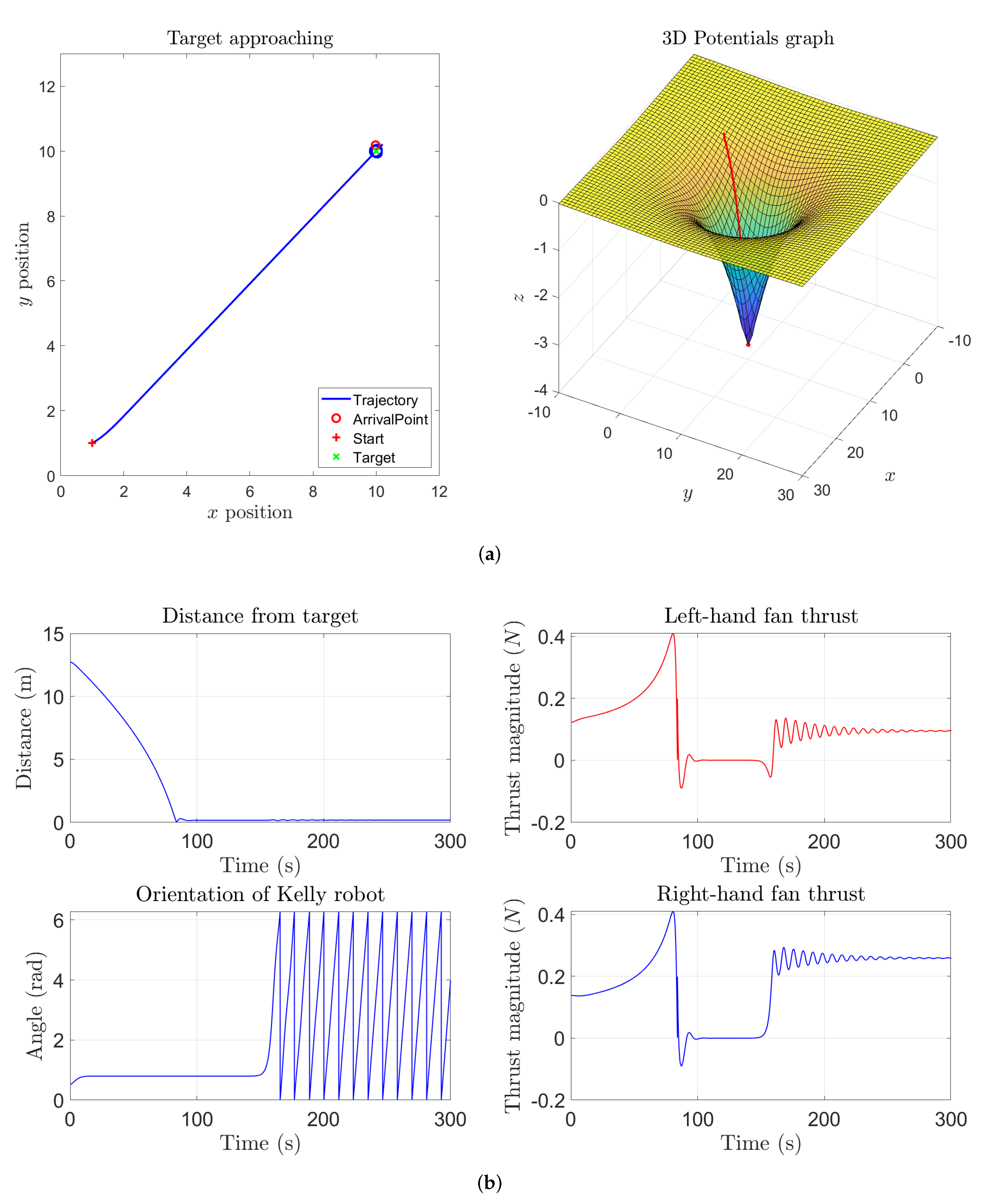
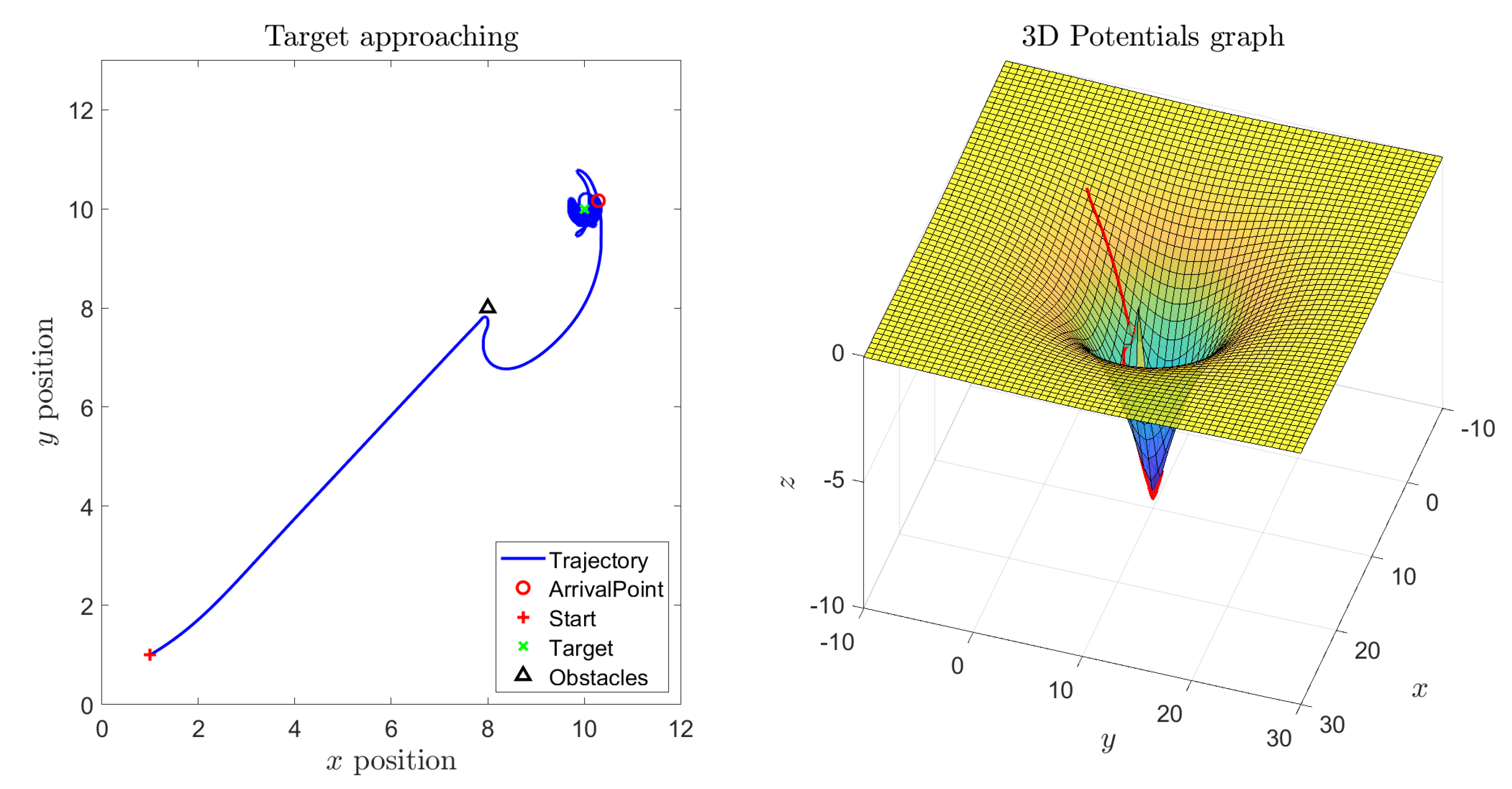
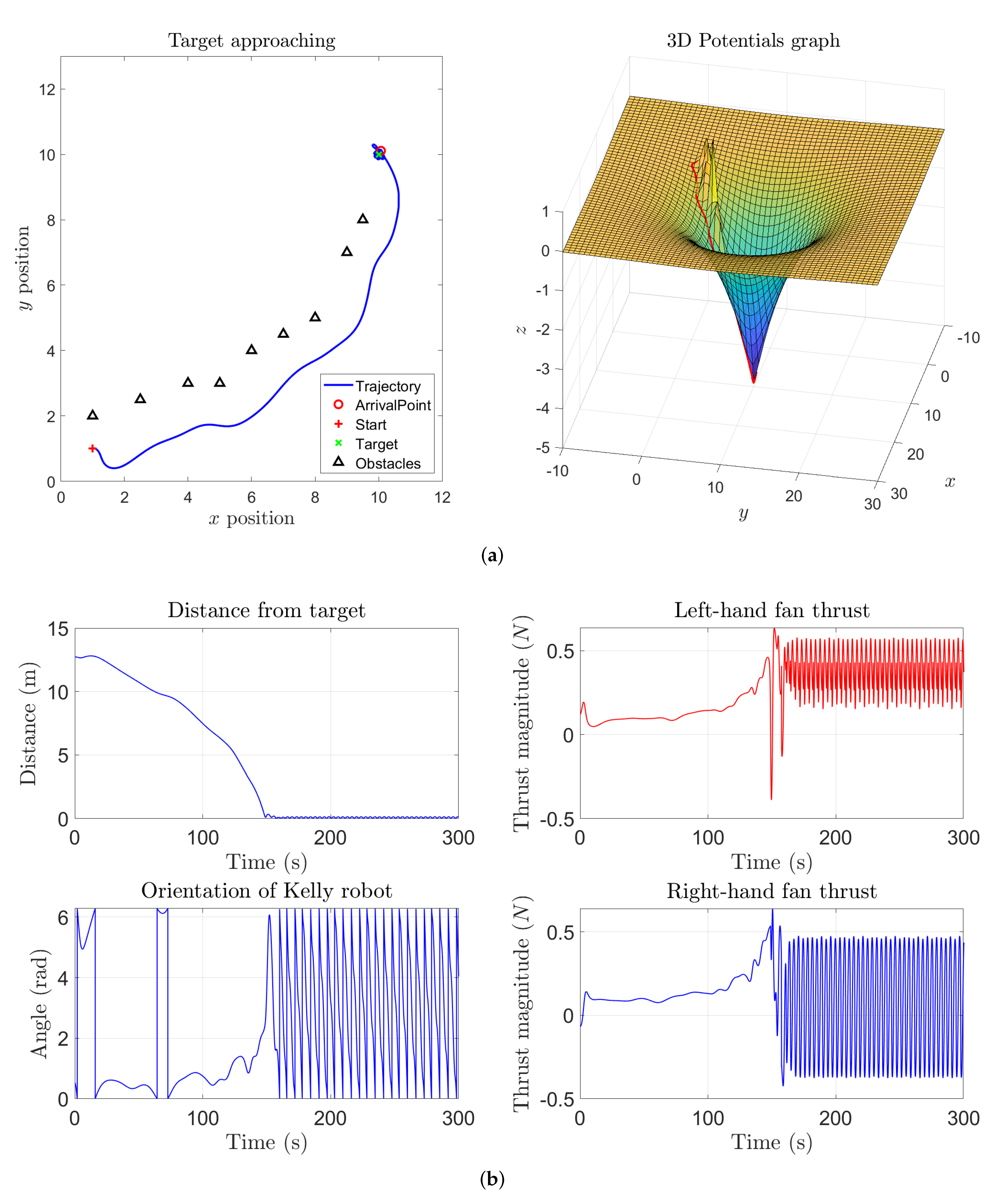
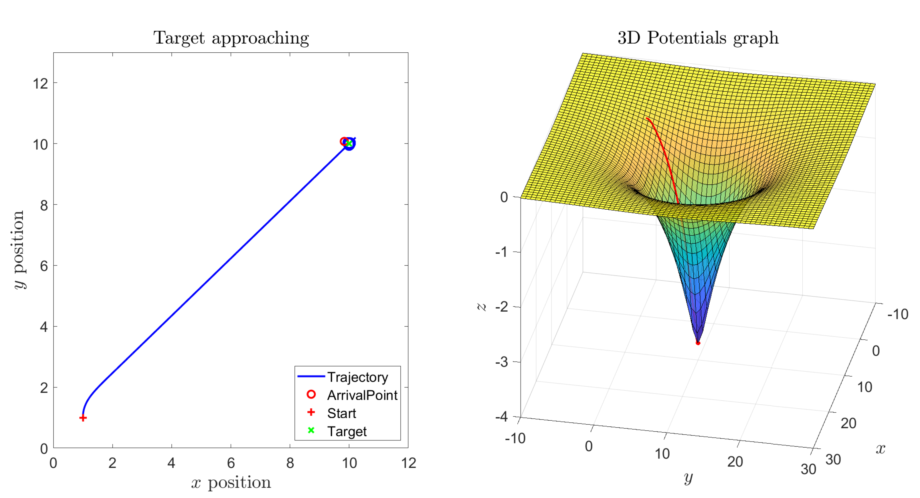
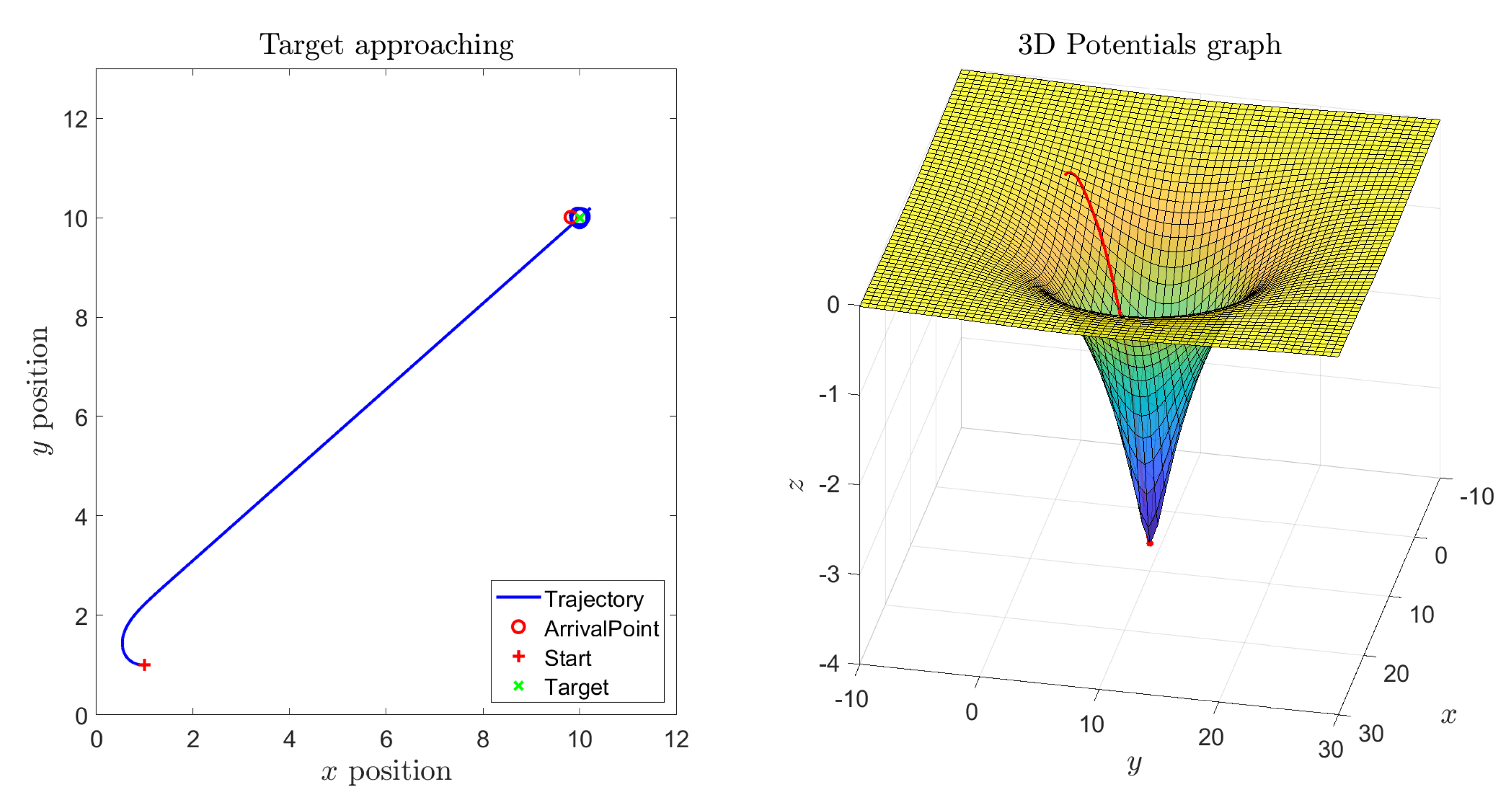
Figure 2 shows the result of a numerical simulation referred to a single target point and no obstacles. From the six panels of such figure it may be readily recognized that the robot traverses the state space from the initial point directly to the target. After the Kelly robot reaches the target, it keeps revolving around the way-point due to the action of the self-propelling term. During vehicle’s journey, the thrusts generated by the left-hand fan and by the right-hand fan look in sync, because the vehicle travels along a straight line, and the orientation of the vehicle keeps almost constant until it reaches the target.

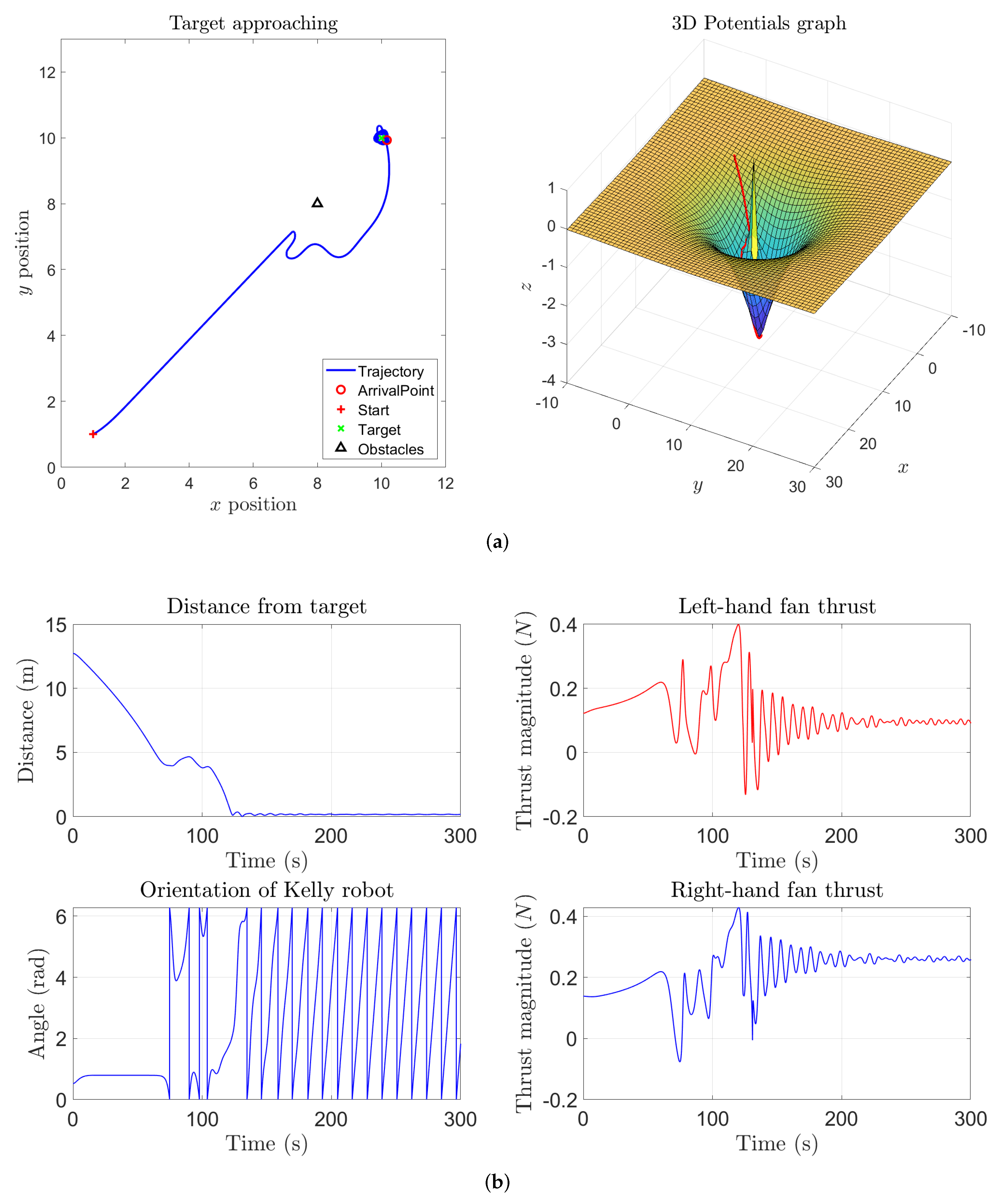
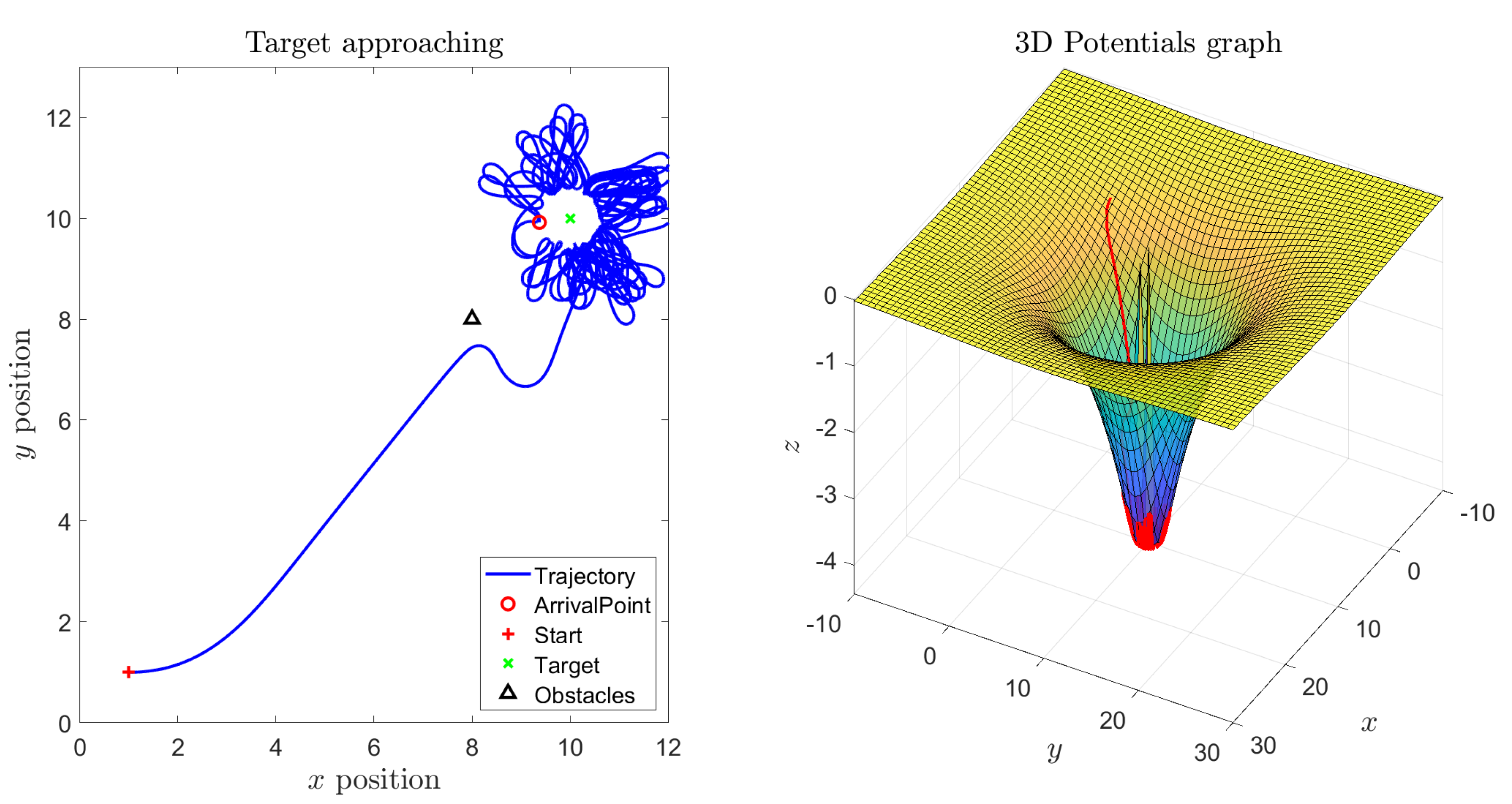
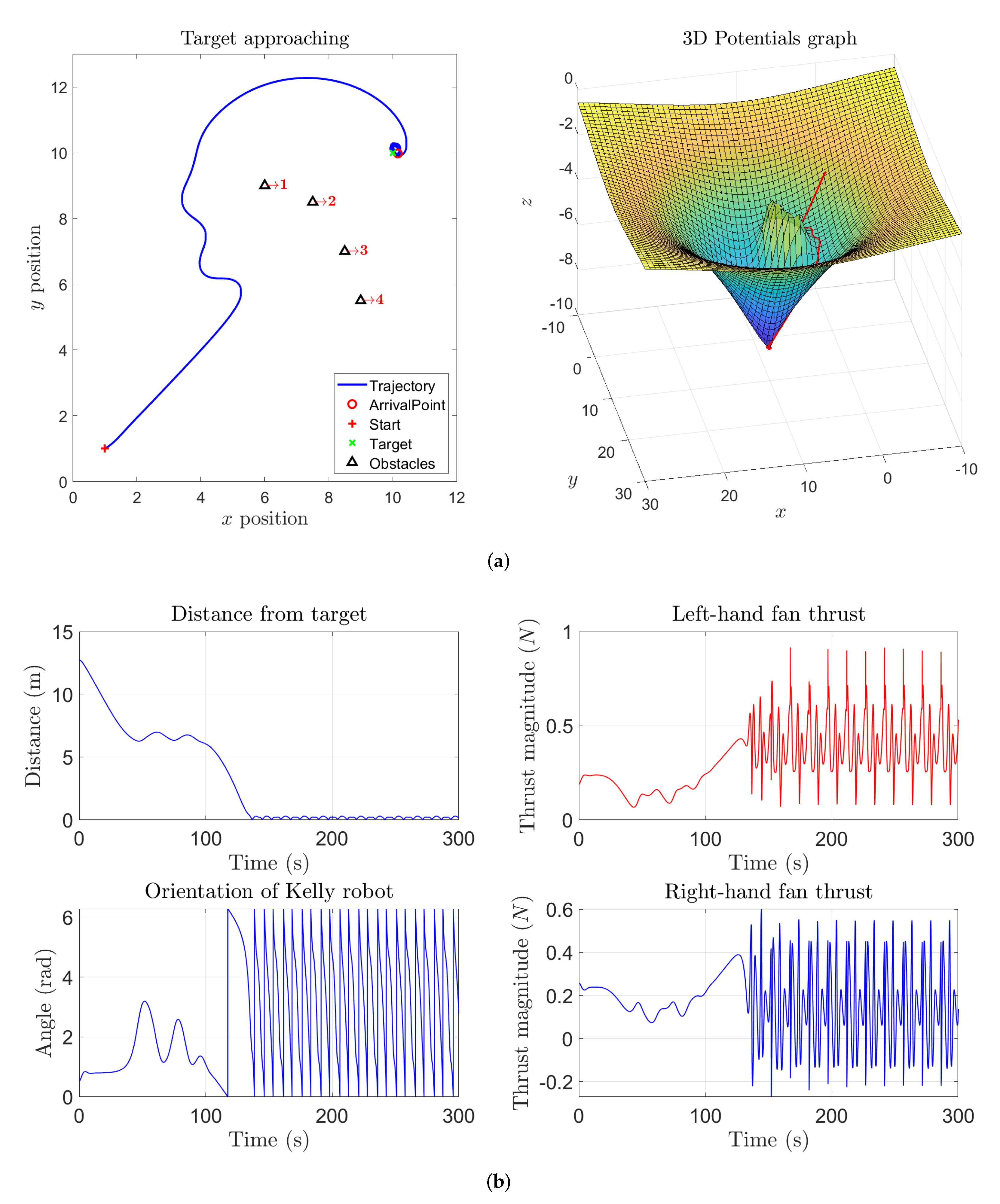
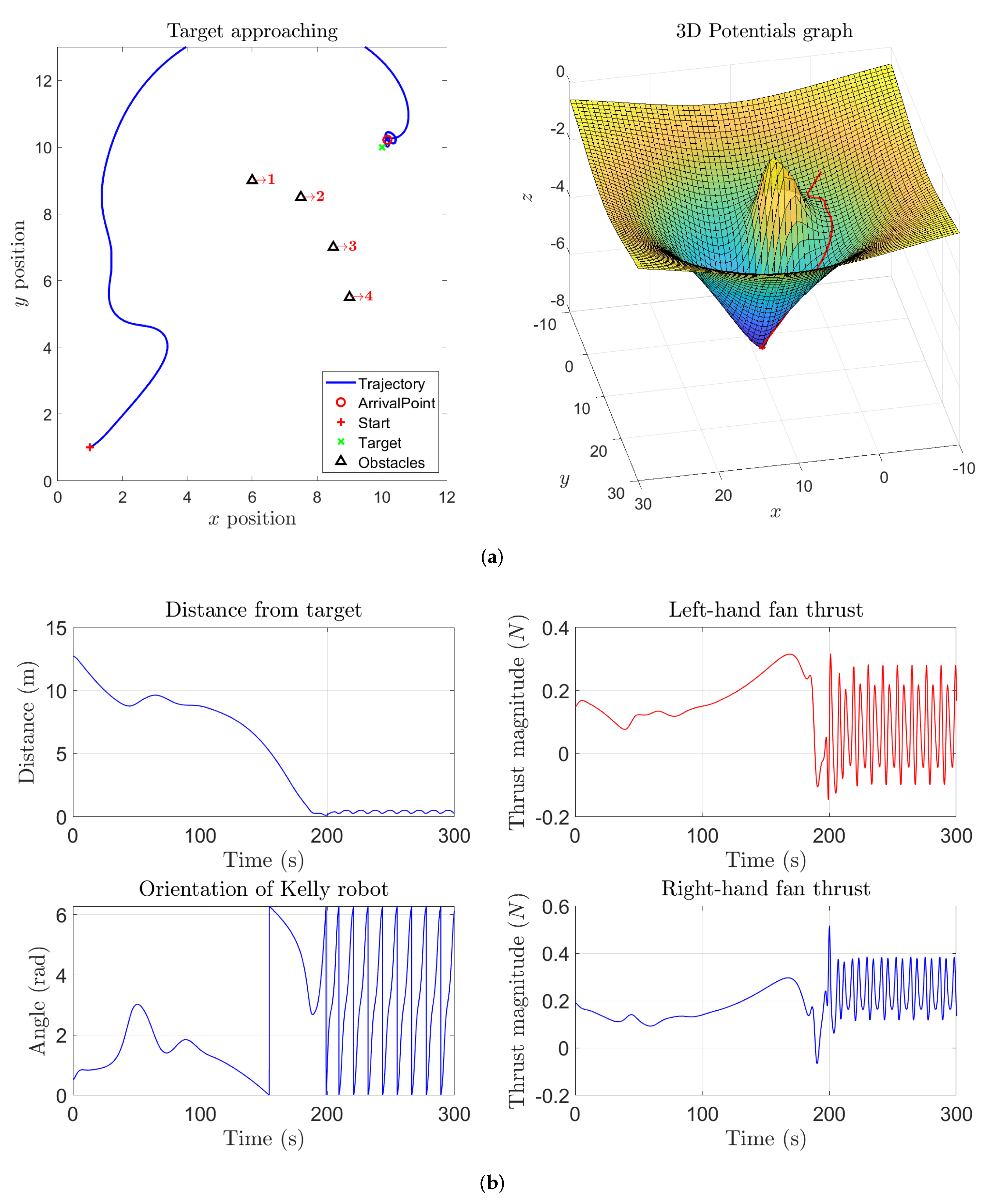
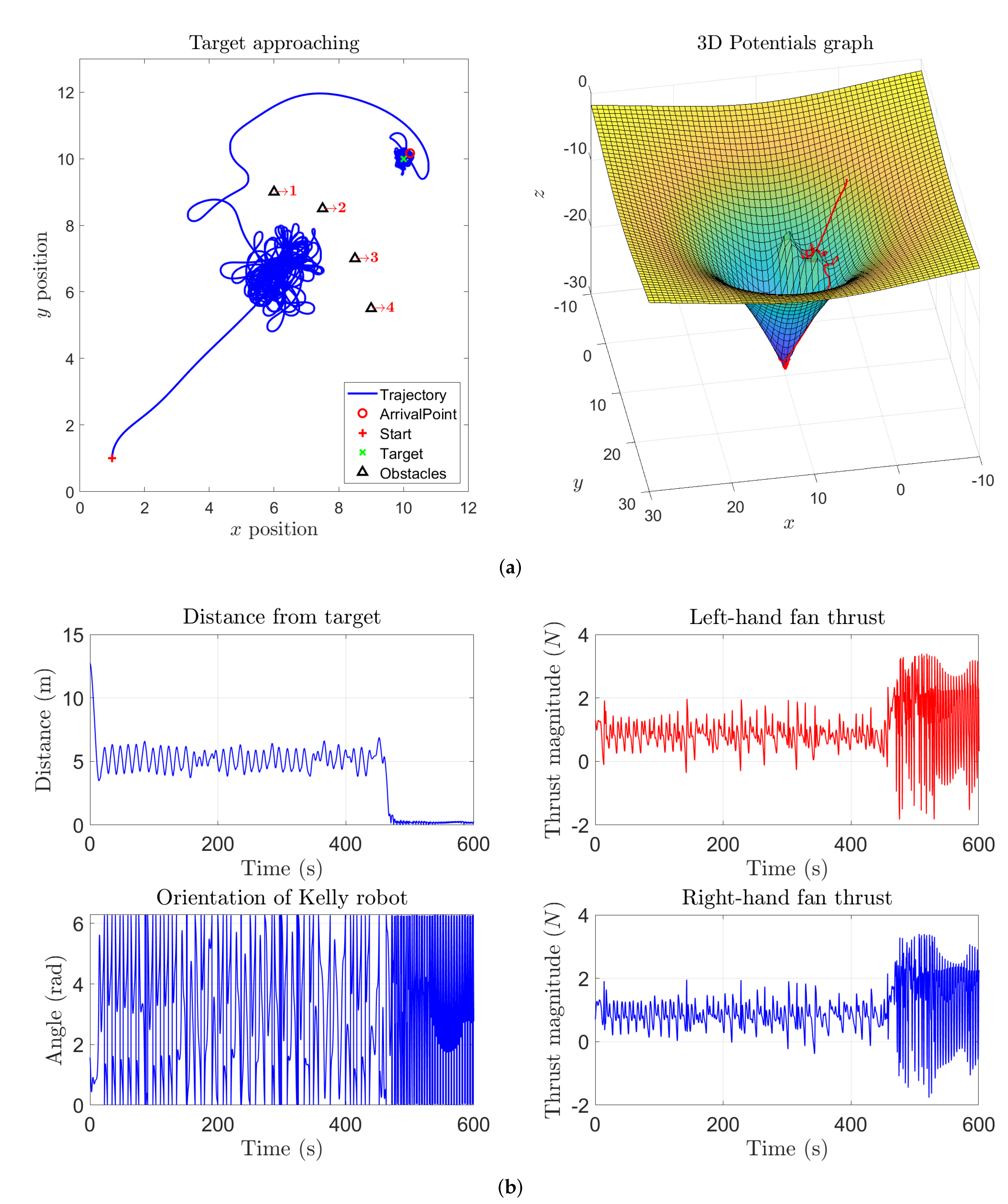
In the next two simulations, an obstacle between the initial location and the target location was added. From Figure 3 it is readily observed how the robot could reach the target and managed to avoid the obstacle. In particular, while the vehicle is located sufficiently far away from the target to ignore its repulsive action, its trajectory resembles a straight line. As soon as the vehicle enters the sphere of influence of the obstacle, its trajectory bends to the left, which corresponds to a sudden increase of the thrust exerted by the right-hand fan around $t=200$ s, to get around the obstacle. After reaching the target, both thrusts stabilize around a value giving rise to a forcing action necessary to counter-act the self-propelling term. Figure 4 shows a result obtained under the same conditions of Figure 3 except that the magnitude of the self-propelling term was increased. In this case, the thrust is quite large, hence the vehicle approaches the target location quickly except then starting to revolve around the target in a pronounced way. Such effect is well visible because the self-propelling term prevails over the attraction pull of the target. Nevertheless, despite the overly irregular movement of the vehicles, the robot draws circular revolving trajectories around the target point.

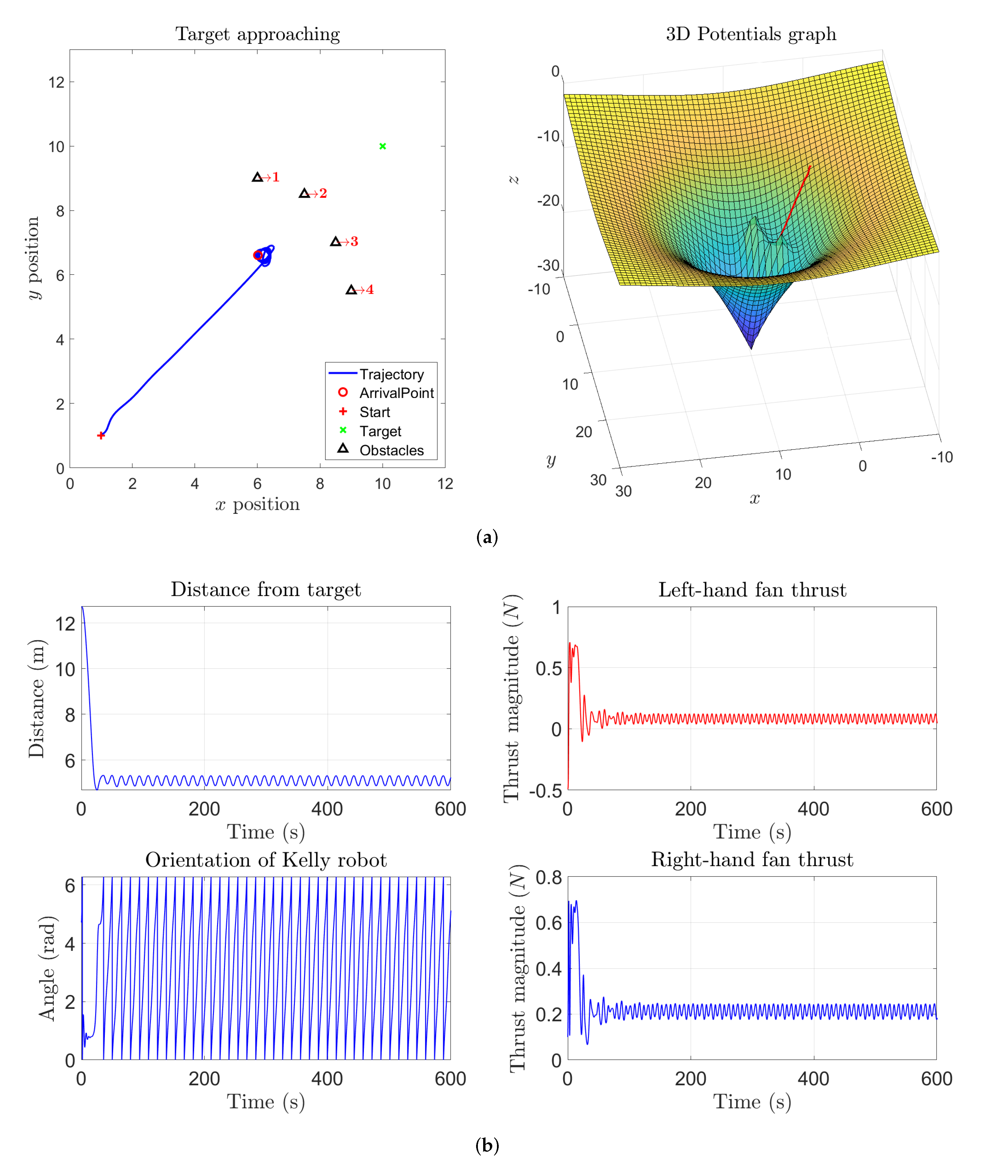
The trajectory followed by a vehicle under the control action of a VARP-based algorithm may be smoothed out by increasing the attractive magnitude of the target to counteract the self-propelling term, as illustrated in Figure 5. Although the robot appears to reach and then wander around the target point, with such a large value of the parameter $\alpha$, it is necessary to consider carefully the irregular trend of the thrusts generated by the propellers. Experimental results show that the self-propelling term must range from $0.1$ to $0.5$ in order to induce a reasonable trajectory on the vehicle: the higher the value of the self-propelling amplitude $\alpha$, the higher the average thrust required to the ducted fans.

A further interesting experiment consisted in building a ‘barrier’ between the starting point and the target location. A barrier, in this context, is constructed by placing a number of obstacles represented by repulsive potentials. Figure 6 shows the results of such numerical experiment. From the 3D potentials graph, it can be readily noticed a potential ‘bulge’ that represents the repulsive influence of the obstacles in the barrier. Even in such a case, a vehicle controlled by a VARP algorithm manages to reach the target location by getting around the barrier.

It can be noticed from Figure 7 that, if a larger value of the parameter ${\ell }_r^{\mathrm{O}}$ is set, the Kelly robot tends to follow a wider trajectory since the obstacles result to be more cumbersome and their influence, in terms of repulsive potentials, is perceived farther by the robot’s control system. The 3D graph displayed in such figure shows how the virtual potential field influences the vehicle in every point of its state space. Indeed, the areas where the repulsive potentials are located correspond to a cumbersome ‘bulge’ in the 3D potentials graph. Compared to Figure 6, the ‘bulge’ appears wider and taller since the repulsive range of obstacles takes a larger value. Instead, the attractive potential corresponding to the target location may be visualized as a depression/dip in the same 3D graph.

In general, the larger the value of the repulsive range, the wider the influence of the obstacles, which could be visualized as wider ‘bulges’ in the potential surface.

Upon choosing, instead, lower values for the repulsive range of the potentials describing the barrier obstacles, a vehicle tends to approach the barrier while, being attracted by the target and as well as being repelled from the obstacles, it might get trapped near the barrier as testified by the numerical experimental result illustrated in Figure 8. It can be noticed from the 3D potentials graph that the vehicle is trapped behind the ‘bulge’ which appears to be less tall than in the previous experiments, since the repulsive range of obstacles takes a lower value. In this case, in order to make a robot be able to overcome the barrier, it is advisable to choose a large value of the self-propelling term coefficient as illustrated by the results displayed in Figure 9.

The previous simulations illustrated cases of study with a few obstacles and one target point. Building a more complex virtual potential field on the basis of more obstacles and/or more targets could lead to a more involved control algorithm yet to a more precise control action on a moving vehicle. As an instance, Figure 10 illustrates how to make a vehicle follow a previously planned path. In such numerical experiment, a vehicle reaches the prescribed target by following a ‘guiding wall’ built through virtual potentials. It is remarkable how, in such simulated experiment, the thrusts exerted by the propellers on the vehicle’s body keep limited in amplitude until the vehicle reaches the target location.

Further simulations were performed by considering different initial orientations of a moving vehicle. Even in these cases, the control algorithm is able to steer the robot towards the prescribed target. Results of numerical simulations are illustrated in Figure 11, Figure 12, Figure 13 and Figure 14. From the results illustrated in Figure 11, in particular, it may be noticed that the Kelly robot reaches the prescribed target without any difficulty and without any particular effort required to the propellers, as testified by the results shown in the panels about the thrusts exerted by the fans, which exhibit a rather regular course over time. In addition, the results displayed in Figure 14 may be compared to the simulation results shown in Figure 13; it is interesting to notice that, in this case, the Kelly robot will turn counterclockwise in order to steer towards the target. This aspect could also be noticed from the Kelly robot orientation graph where the plot reaches $2\pi$ and suddenly drops to 0.

The numerical simulations presented in this section are meaningful in view of an extension of the standard VARP control theory to state manifolds and serve as a guide in the development of illustrative numerical experiments concerning the next part of the paper. In fact, the large number of numerical results were designed to gain (and to guide readers through) a deeper understanding about the effects of the values of the parameters on the control outcomes.

As mentioned in the Introduction, the pursued extension of the VARP theory to state manifolds was partially inspired by the earlier work of Koditschek and Rimon [16], which however considered simpler gradient systems and was more theoretical-oriented (in particular, the work [16] is notable for the use of topological arguments to prove the existence of navigation functions on a large class of manifolds).

Notice that all the obstacles located in have been supposed to be stationary, although this is not a strict requirement for the devised theory to hold.

4. Extension of the VARP Control Theory to Riemannian Manifolds

The aim of the present section is to design a VARP-like principle to control second-order dynamical systems whose state space is a Riemannian manifold. This method will be referred to as M-VARP as it represents an extension of the original VARP control method to a generic Riemannian manifold.

A number of real-world dynamical systems may be framed as systems on manifolds. An example is a flying drone or an orbital gyrostat whose attitude is represented by a special orthogonal matrix belonging to a manifold denoted as SO(3) as illustrated, for example, in [41,42,43].

Successively, the devised M-VARP principle will be implemented and simulated for the case of study where it controls an abstract dynamical system whose state space is the sphere ${\mathbb{S}}^2$ (which will be denoted as ${\mathbb{S}}^2$-VARP). As in the previous experiments, we shall consider the presence of a single agent (as a matter of fact, in this paper we do not deal with ‘cooperative control’). As a general reference to manifold calculus, interested readers might want to refer to the Symmetry tutorial paper [40].

4.1. Generalities on Riemannian Manifolds

Let $\mathbb{M}$ denote a smooth manifold. At a point $x\in \mathbb{M}$, the tangent space to the manifold $\mathbb{M}$ is denoted as $T_x\mathbb{M}$. The symbol $T\mathbb{M}$ denotes the tangent bundle associated to the manifold $\mathbb{M}$ defined as $T\mathbb{M}:=\{(x,v)\mid x\in \mathbb{M},v\in T_x\mathbb{M}\}$.

A Riemannian manifold $\mathbb{M}$ is endowed with a bilinear, positive-definite form ${\langle ·,·\rangle }_x:T_x\mathbb{M}\times T_x\mathbb{M}\to \mathbb{R}$ that associates a scalar (or inner) product to each tangent space $T_x\mathbb{M}$. A local metric ${\langle ·,·\rangle }_x$ also defines a local norm ${\parallel v\parallel }_x:=\sqrt{{\langle v,v\rangle }_x}$, for $v\in T_x\mathbb{M}$.

The Riemannian gradient of a scalar-valued function $\psi :\mathbb{R}\to \mathbb{M}$ evaluated at a point $x\in \mathbb{M}$ is denoted as ${\mathrm{grad}}_x\psi$. The Riemannian gradient is associated to a specific metric.

A manifold exponential map $exp:T\mathbb{M}\to \mathbb{M}$ maps a pair $(x,v)\in T_x\mathbb{M}$ to a point $y={exp}_x\left(v\right)$ on the manifold. The exponential map ‘shifts’ a point x along a geodesic curve in the direction of v to get to the point y. Its inverse ‘log’ is defined only locally and is termed manifold logarithm. Given points $x,y\in \mathbb{M}$, a manifold logarithm computes a tangent vector $v={log}_x\left(y\right)\in T_x\mathbb{M}$ such that ${exp}_x\left(v\right)=y$.

Given two points $x,y\in \mathbb{M}$ connectable by a geodesic arc, their Riemannian distance is denoted by $d(x,y)$. On a Riemannian manifold, the distance between two nearby points may be evaluated by:

$$d(x,y)=\parallel {log}_x{\left(y\right)\parallel }_x.$$

(33)

A fundamental result of the calculus on manifolds states that the Riemannian gradient of a squared distance function reads:

$${\mathrm{grad}}_x{d}^2(x,y)=-2{log}_x\left(y\right),$$

(34)

wherever the logarithm is defined (for a proof, see, e.g., [40]).

The covariant derivative, a generalization of directional derivative of calculus, of a vector field $w_x\in T_x\mathbb{M}$ in the direction of a vector $v\in T_x\mathbb{M}$ is denoted as ${\nabla }_{v}w$. We assume $\mathbb{M}$ to be endowed with a metric connection (namely, that the covariant derivative of the metric tensor is identically zero).

The parallel transport operator $\mathrm{P}:T{\mathbb{M}}^2\to T\mathbb{M}$ maps a tangent vector $v\in T_x\mathbb{M}$ at a given point $x\in \mathbb{M}$ into a tangent vector $w\in T_y\mathbb{M}$ at another given point $y\in \mathbb{M}$, which is denoted as $w={\mathrm{P}}^{x\to y}\left(v\right)$. Parallel transport moves the tangent vector v from $T_x\mathbb{M}$ to $T_y\mathbb{M}$ along the geodesic curve that connects the point x to the point y (if any) preserving its tangency along the geodesic arc and the angle formed to the tangent to the geodesic, in such a way to realize a conformal isometry.

Parallel transport and covariant derivation are closely related to one another, in particular, covariant derivation may be expressed in terms of parallel transport as follows:

$${\left({\nabla }_{v}w\right)}_x=\underset{h\to 0}{lim}\frac{{\mathrm{P}}^{\gamma \left(h\right)\to x}\left(w_{\gamma \left(h\right)}\right)-w_x}{h},$$

(35)

where $\gamma$ denotes any smooth curve with prescribed foot-point and direction, namely such that $\gamma \left(0\right)=x\in \mathbb{M}$ and $\dot{\gamma }\left(0\right)=v\in T_x\mathbb{M}$. For practical/computational purposes, such smooth curve is often taken as a geodesic arc. Such relationship leads to a numerical approximation of the covariant derivative at a point x, as it will be pointed out in Section 4.3.

4.2. Extension of the VARP Principle to Riemannian Manifolds

In order to extend the VARP principle to control dynamical systems whose state spaces are Riemannian manifolds, it is necessary to recall a fairly broad class of second-order dynamical systems. In the present context, it is sufficient to take into account a class of second-order dynamical systems whose state-transition equations are formulated on the tangent bundle of a manifold $\mathbb{M}$, described by:

$$\left\{\begin{array}{c}\dot{x}\left(t\right)=v\left(t\right),\hfill \\ {\nabla }_{v\left(t\right)}v\left(t\right)=-\mu v\left(t\right)+u\left(t\right).\hfill \end{array}\right.$$

(36)

In such equations, the following notation has been used:

• the function $x\left(t\right)\in \mathbb{M}$ denotes the state of the dynamical system (it could be thought of as the position of a pointwise mass on the manifold at time t);
• the function $v\left(t\right)\in T_{x\left(t\right)}\mathbb{M}$ denotes the tangent vector to the trajectory $x\left(t\right)$ at the time t (it could be thought of as the velocity of a pointwise mass on the manifold);
• the vector field ${\nabla }_{v}v$ represents the covariant derivative of the vector field v with respect to itself (it could be thought of as the acceleration of the pointwise mass on the manifold); if ${\nabla }_{v}v=0$ the acceleration is zero, thus the pointwise mass will follow a uniform geodesic trajectory (which represents the counterpart, in the ordinary space, of a straight uniform motion);
• the constant $\mu >0$ denotes a ‘viscous’ friction coefficient (therefore, the term $-\mu v$ could be thought of as a friction force which brakes the motion of a pointwise mass sliding over the manifold);
• the function $u\left(t\right)$ denotes a control action at time t (it could be thought of as a force whose purpose is to make a pointwise mass move on a manifold and deviate with respect to a purely geodesic trajectory); such control action is a vector field which is tangent to the manifold at the state $x\left(t\right)$.

On the basis of the above formulation of a dynamical system on manifold, it is viable to extend the VARP control principle recalled in Section 2. In fact, an extension to manifold-type state-space systems of the type (36) consists in setting the control action u according to a manifold-consistent translation of the terms in the VARP principle (3). The proposed extension is outlined in the following:

$$\left\{\begin{array}{c}\dot{x}\left(t\right)=v\left(t\right),\hfill \\ {\nabla }_{v\left(t\right)}v\left(t\right)=-\mu v\left(t\right)+\alpha \widehat{v}\left(t\right)-{\mathrm{grad}}_{x\left(t\right)}V,\hfill \\ V\left(x\right)={\displaystyle \sum _{j=1}^N}\left(V_j^{\mathrm{r}}\left(d^2(x,q_j)\right)-V_j^{\mathrm{a}}\left(d^2(x,q_j)\right)\right).\hfill \end{array}\right.$$

(37)

The terms appearing in the above equations may be explained as follows:

• the term $\alpha \widehat{v}$, with $\alpha >0$, represents a self-propelling term, where $\widehat{v}:=v/\parallel v\parallel$ if $v\ne 0$ otherwise $\widehat{v}=0$;
• the function $V\left(x\right)$ denotes the total potential which depends on the state x; the functions $V_j^{\mathrm{r}}$ and $V_j^{\mathrm{a}}$ denote, respectively, the repulsive and attractive components of the potential function, as they were already defined for Euclidean spaces in Section 2.2; note that the components are indexed by the index j: this indexing does not appear explicitly in [39] while, in the present case, each obstacle and target has its own coefficient;
• the N terms labeled $q_j$ represent obstacle-associated and target-associated locations on the manifold $\mathbb{M}$;
• the function $d^2(·,·)$ denotes the squared Riemannian distance between two points on the state manifold $\mathbb{M}$; notice that, in the equations, it appears squared because such choice, generally, simplifies the calculation of derivatives.

Combining together the Equations (36) and (37), it can be readily seen that the control field u takes the expression:

$$\begin{array}{c}\hfill \begin{array}{cc}\hfill u:=& \alpha \widehat{v}-{\mathrm{grad}}_x\sum _{j=1}^N\left(V_j^{\mathrm{r}}\left(d^2(x,q_j)\right)-V_j^{\mathrm{a}}\left(d^2(x,q_j)\right)\right)=\hfill \\ \hfill =& \alpha \widehat{v}-\sum _{j=1}^N\left({\dot{V}}_j^{\mathrm{r}}\left(d^2(x,q_j)\right)-{\dot{V}}_j^{\mathrm{a}}\left(d^2(x,q_j)\right)\right){\mathrm{grad}}_x{d}^2(x,q_j).\hfill \end{array}\end{array}$$

(38)

Recalling the relationship (34) for Riemannian manifolds leads to the expression:

$$u=\alpha \widehat{v}-2\sum _{j=1}^N\left({\dot{V}}_j^{\mathrm{a}}\left(d^2(x,q_j)\right)-{\dot{V}}_j^{\mathrm{r}}\left(d^2(x,q_j)\right)\right){log}_x\left(q_j\right),$$

(39)

where ${\dot{V}}_j^{\mathrm{a}}:=\frac{\mathrm{d}{V}_j^{\mathrm{a}}\left(\varphi \right)}{\mathrm{d}\varphi }$ and ${\dot{V}}_j^{\mathrm{r}}:=\frac{\mathrm{d}{V}_j^{\mathrm{r}}\left(\varphi \right)}{\mathrm{d}\varphi }$.

Coherently with what was expected, the results show that $u\in T_x\mathbb{M}$.

In analogy to the VARP principle formulated on Euclidean spaces (see Equation (4)), exponential-type attractive and repulsive potential functions have been chosen as:

$$V_j^{\mathrm{a}}\left(\varphi \right):=C_j^{\mathrm{a}}{e}^{-\sqrt{\varphi }/{\ell }_j^{\mathrm{a}}},V_j^{\mathrm{r}}\left(\varphi \right):=C_j^{\mathrm{r}}{e}^{-\sqrt{\varphi }/{\ell }_j^{\mathrm{r}}},$$

(40)

where $C_j^{\mathrm{a}}$ and $C_j^{\mathrm{r}}$ denote the ‘magnitude of the potentials’, ${\ell }_j^{\mathrm{a}}$ and ${\ell }_j^{\mathrm{r}}$ their ‘characteristic lengths’ and $\varphi$ denotes a real positive variable. Their derivatives with respect to $\varphi$ take the expressions:

$$\frac{\mathrm{d}{V}_j^{\mathrm{a}}\left(\varphi \right)}{\mathrm{d}\varphi }=-\frac{C_j^{\mathrm{a}}}{2{\ell }_j^{\mathrm{a}}\sqrt{\varphi }}{e}^{-\sqrt{\varphi }/{\ell }_j^{\mathrm{a}}},\frac{\mathrm{d}{V}_j^{\mathrm{r}}\left(\varphi \right)}{\mathrm{d}\varphi }=-\frac{C_j^{\mathrm{r}}}{2{\ell }_j^{\mathrm{r}}\sqrt{\varphi }}{e}^{-\sqrt{\varphi }/{\ell }_j^{\mathrm{r}}},$$

(41)

therefore the control field (39) ultimately reads:

$$u\left(t\right)=\alpha \widehat{v}\left(t\right)-\sum _{j=1}^N\left(\frac{C_j^{\mathrm{r}}}{{\ell }_j^{\mathrm{r}}}\frac{e^{-d(x\left(t\right),q_j)/{\ell }_j^{\mathrm{r}}}}{d(x\left(t\right),q_j)}-\frac{C_j^{\mathrm{a}}}{{\ell }_j^{\mathrm{a}}}\frac{e^{-d(x\left(t\right),q_j)/{\ell }_j^{\mathrm{a}}}}{d(x\left(t\right),q_j)}\right){log}_{x\left(t\right)}\left(q_j\right).$$

(42)

The M-VARP-controlled dynamical system (in analogy to a VARP-controlled Kelly robot described in Section 3.2) is hence described by the following system of equations:

$$\left\{\begin{array}{c}\dot{x}\left(t\right)=v\left(t\right),\hfill \\ \begin{array}{cc}\hfill {\nabla }_{v\left(t\right)}v\left(t\right)=& -\mu v\left(t\right)+\alpha \widehat{v}\left(t\right)\hfill \\ \hfill & -\sum _{j=1}^N\left(\frac{C_j^{\mathrm{r}}}{{\ell }_j^{\mathrm{r}}}\frac{e^{-d(x\left(t\right),q_j)/{\ell }_j^{\mathrm{r}}}}{d(x\left(t\right),q_j)}-\frac{C_j^{\mathrm{a}}}{{\ell }_j^{\mathrm{a}}}\frac{e^{-d(x\left(t\right),q_j)/{\ell }_j^{\mathrm{a}}}}{d(x\left(t\right),q_j)}\right){log}_{x\left(t\right)}\left(q_j\right).\hfill \end{array}\hfill \end{array}\right.$$

(43)

The first equation governs the evolution of the state x of the dynamical system on the basis of its (tangent) velocity v, while the second equation governs the evolution of the velocity on the basis of the chosen potentials, of the state and of the state-velocity itself. Notice that again all the obstacles located in $q_j$ have been supposed to be stationary, although this is not a strict requirement for the devised theory to hold.

4.3. Extended Euler Scheme for the Numerical Simulation of the M-VARP Control Method

In the preset subsection, we shall illustrate an extension of the previously-recalled forward Euler method to numerically simulate a controlled system on manifold.

The system (43) to be simulated numerically may be recast in compact form as:

$$\left\{\begin{array}{c}\dot{x}\left(t\right)=v\left(t\right),\hfill \\ {\nabla }_{v\left(t\right)}v\left(t\right)=\sigma (x\left(t\right),v\left(t\right)),\hfill \\ x\left(0\right)=x^0,v\left(0\right)=v^0\left(initialconditions\right),\hfill \end{array}\right.$$

(44)

where $\sigma :T\mathbb{M}\to T\mathbb{M}$ is the function on the right-hand side of the second equation in (43) that maps a point x and a tangent vector $v\in T_x\mathbb{M}$ into a tangent vector in $T_x\mathbb{M}$.

To solve numerically the system of differential Equation (44), namely to simulate the controlled system (43), we introduce three discrete-time sequences that arise from time discretization with a step size $h>0$:

• the sequence $x^k\in \mathbb{M}$, with $k=0,1,2,3,\dots$, represents a time-discretized version of the state $x\left(t\right)$, namely $x^k$ denotes a numerical approximation of the exact state $x\left(kh\right)$;
• the sequence $v^k\in \mathbb{M}$, with $k=0,1,2,3,\dots$, represents a time-discretized version of the velocity $v\left(t\right)$, namely $v^k$ denotes a numerical approximation of the exact state-velocity $v\left(kh\right)$;
• the sequence $u^k\in \mathbb{M}$, with $k=0,1,2,3,\dots$, represents a time-discretized version of the control field $u\left(t\right)$, namely $u^k$ denotes a numerical approximation of $u\left(kh\right)$, that is:

  $$u^k:=\alpha {\widehat{v}}^k-\sum _{j=1}^N\left(\frac{C_j^{\mathrm{r}}}{{\ell }_j^{\mathrm{r}}}\frac{e^{-d(x^k,q_j)/{\ell }_j^{\mathrm{r}}}}{d(x^k,q_j)}-\frac{C_j^{\mathrm{a}}}{{\ell }_j^{\mathrm{a}}}\frac{e^{-d(x^k,q_j)/{\ell }_j^{\mathrm{a}}}}{d(x^k,q_j)}\right){log}_{x^k}\left(q_j\right).$$

  (45)

Notice that the discrete-time index is denoted by a superscript (${}^k$) to avoid confusing it with the obstacle/target index which is denoted by subscript (${}_j$). Once a time discretization of the variables that describe the state of a dynamical system has been performed, an extension of the forward Euler method (fEul) to manifolds may be devised. To express such fEul-like method, the exponential map and the parallel transport operators recalled in Section 4.1 shall be invoked.

As a further consideration that motivates the usage of a simple numerical scheme, such as the forward Euler one, when more precise schemes are available (such as the ones in the Runge–Kutta class), we notice that such higher-order schemes would require evaluating the control field in points of the trajectory that are not available within the numerical schemes, hence causing additional computational efforts and accumulation of additional numerical errors.

It is important to remind that the parallel transport operator is fundamental in the calculation of the covariant derivative. Let us denote by $w_x$ a vector field on $T\mathbb{M}$ (in each point x of the manifold, $w_x$ defines a tangent vector at x) of which the covariant derivative is sought, and by $v_x$ another vector field along which such covariant derivative needs to be calculated. The sought covariant derivative is then defined as:

$${\left({\nabla }_{v}w\right)}_x=\underset{h\to 0}{lim}\frac{w_{{exp}_x\left(h{v}_x\right)}-{\mathrm{P}}^{x\to {exp}_x\left(h{v}_x\right)}\left(w_x\right)}{h}.$$

(46)

Indeed, the covariant derivative ${\left({\nabla }_{v}w\right)}_x$ represents the rate of change of the vector field w along the direction prescribed by the vector field v, namely, moving away from x toward a direction v.

Let us consider numerical resolution of the first equation in (44) that is:

$$\frac{\mathrm{d}x\left(t\right)}{\mathrm{d}t}=v\left(t\right),x\left(0\right)=x^0\in \mathbb{M},$$

(47)

which is an IVP on the tangent bundle $T\mathbb{M}$. An algorithm that implements the numerical solution in a fEul-like fashion reads:

$$x^{k+1}={exp}_{x^k}\left(h{v}^k\right),k=0,1,2,3,\dots ,$$

(48)

with $x^0$ and $v^0$ known from the initial conditions.

Let us consider now numerical resolution of the second equation of (44), that is:

$${\nabla }_{v\left(t\right)}v\left(t\right)=\sigma (x\left(t\right),v\left(t\right)),v\left(0\right)=v^0\in T_{x^0}\mathbb{M},$$

(49)

which represents a further IVP on the tangent bundle $T\mathbb{M}$.

The relation (46), applied to the vector field v with respect to itself, could be numerically approximated as:

$${\nabla }_{v\left(hk\right)}v\left(hk\right)\approx \frac{v^{k+1}-{\mathrm{P}}^{x^k\to x^{k+1}}\left(v^k\right)}{h}.$$

(50)

(We notice that the above relationship is somewhat arbitrary, albeit natural. In fact, the quantities $x^{k+1}$ and $v^{k+1}$ are not related to the quantities $x^k$ and $v^k$ as much as in the exact relationship (46) and, in particular, are not related to h by a straighforward relationsip, hence the division by h may appear somewhat arbitrary.) Therefore, an algorithm that implements the numerical solution of (49) in a fEul-like fashion reads:

$$v^{k+1}={\mathrm{P}}^{x^k\to x^{k+1}}(v^k+h\sigma (x^k,v^k)),k=0,1,2,3,\dots ,$$

(51)

with $x^0$ and $v^0$ known from the initial conditions.

In summary, the numerical iteration that will be made use of in order to simulate a controlled second-order system on manifold reads:

$$\left\{\begin{array}{c}{x}^{k+1}={exp}_{x^k}\left(h{v}^k\right),\hfill \\ u^k=\alpha {\widehat{v}}^k-\sum _{j=1}^N\left(\frac{C_j^{\mathrm{r}}}{{\ell }_j^{\mathrm{r}}}\frac{e^{-d(x^k,q_j)/{\ell }_j^{\mathrm{r}}}}{d(x^k,q_j)}-\frac{C_j^{\mathrm{a}}}{{\ell }_j^{\mathrm{a}}}\frac{e^{-d(x^k,q_j)/{\ell }_j^{\mathrm{a}}}}{d(x^k,q_j)}\right){log}_{x^k}\left(q_j\right),\hfill \\ v^{k+1}={\mathrm{P}}^{x^k\to x^{k+1}}\left((1-h\mu )v^k+h{u}^k\right),\hfill \\ k=0,1,2,3,\dots ,\hfill \end{array}\right.$$

(52)

with $x^0$ and $v^0$ known from the initial conditions.

In the following section, numerical results will illustrate a number of features of the devised control strategy on manifold, with reference to the unit hyper-sphere as exemplary case. Let us recall that, in the case of hyper-sphere ($\mathbb{M}:={\mathbb{S}}^{n-1}$), the canonical operators and the Riemannian distance required for the numerical implementation take the following expressions:

$$\left\{\begin{array}{c}{exp}_x\left(v\right)=\left\{\begin{array}{c}xcos(\parallel v\parallel )+{v\parallel v\parallel }^{-1}sin(\parallel v\parallel ),ifv\ne 0,\hfill \\ x,\mathrm{otherwise},\hfill \end{array}\right.\hfill \\ d(x,y)=|arccos\left(x^{\top }y\right)|,\hfill \\ {log}_{x}y=\frac{d(x,y)}{sind(x,y)}(I_n-x{x}^{\top })y,\hfill \\ {\mathrm{P}}^{x\to y}\left(v\right)=\left[I_n-\frac{(y+x)y^{\top }}{1+x^{\top }y}\right]v.\hfill \end{array}\right.$$

(53)

The expression given about the logarithmic map is continuous in $x=y$, in fact it is easily seen that:

$$\underset{d(x,y)\to 0}{lim}\frac{d(x,y)}{sind(x,y)}(I_n-x{x}^{\top })y=0.$$

In the expression of parallel transport, it is understood that points x and y need not be antipodal, namely $x^{\top }y\ne -1$.

4.4. Simulations Results about the ${\mathbb{S}}^2$-VARP Method

In the present subsection, results of numerical simulations will be reported in order to illustrate salient features of the M-VARP control method on the unitary sphere ${\mathbb{S}}^2$. The values of the parameters displayed in the figure captions were determined on the basis of a trial-and-error procedure, since the non-linear control algorithm is not prone to theoretical determination of optimal coefficients in any analytic way. Notice that in an abstract system the ‘temporal’ parameter t is immaterial, hence the duration of each numerical simulation is expressed in terms of computing steps. The value of the chosen numerical stepsize in every simulation in this section is $h=0.01$ (s).

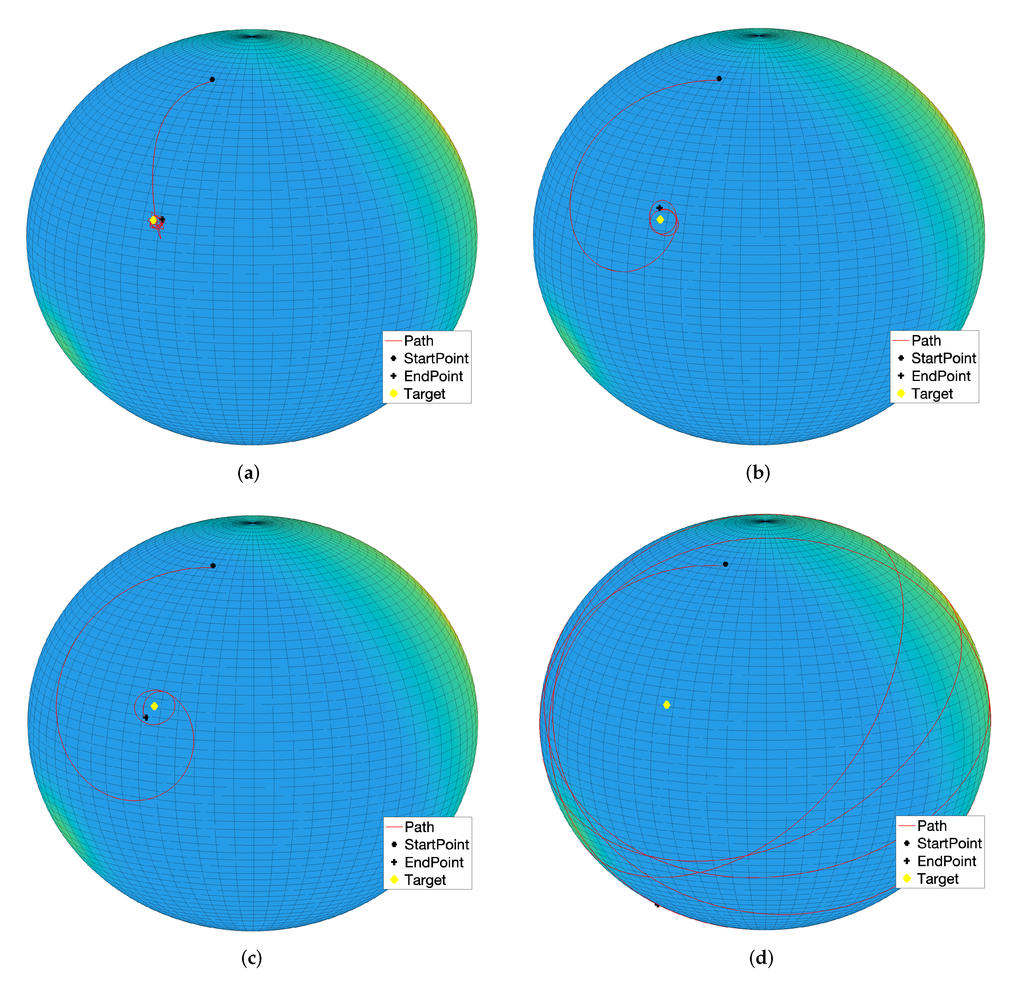
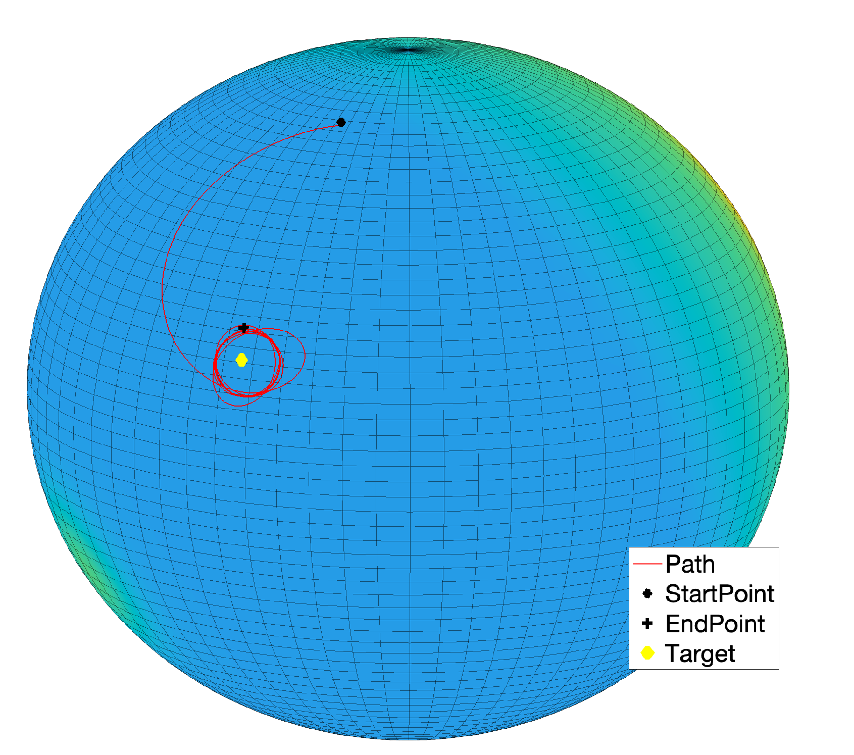
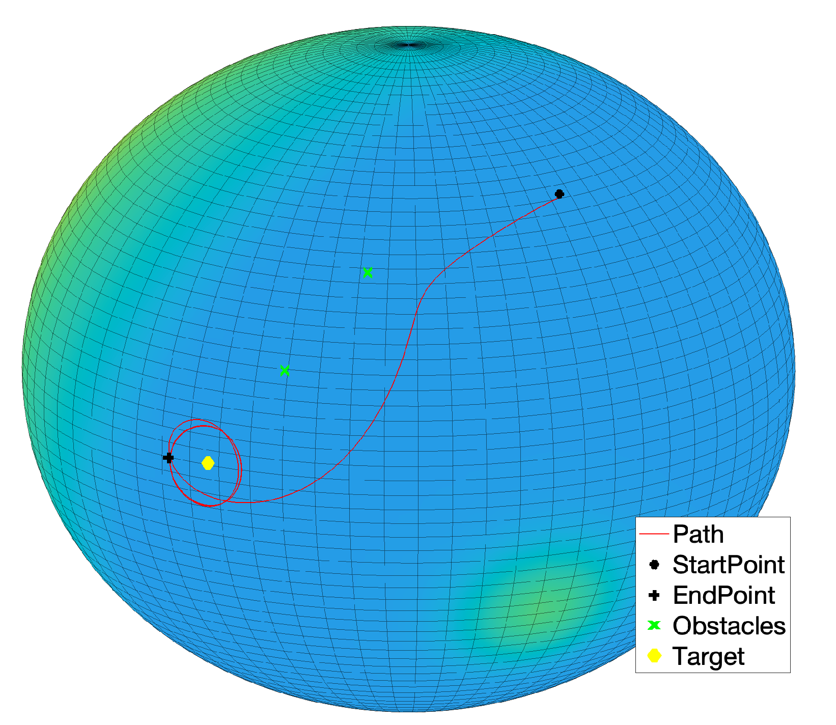
The first five numerical simulation results concern a case study where a single target is present while no obstacles were placed over the sphere. Figure 15a shows the state trajectory followed by an abstract second-order dynamical system on the sphere and, as expected, the system state reaches the prescribed target. Across the following subfigures, the self-propelling coefficient was gradually increased, which explains why the system gradually follows a wider path, as illustrated in Figure 15b,c. With an higher value of the coefficient $\alpha$, self-propulsion is stronger than the attractive influence of the target, hence the system state will wander around the sphere without ever reaching the target, as displayed in Figure 15d. However, by increasing the attractive magnitude of the target ($C_a^{\mathrm{T}}=7$), the attractive potential is able to counteract the self-propelling term in order to make the system state reach the target again, as shown in Figure 16.

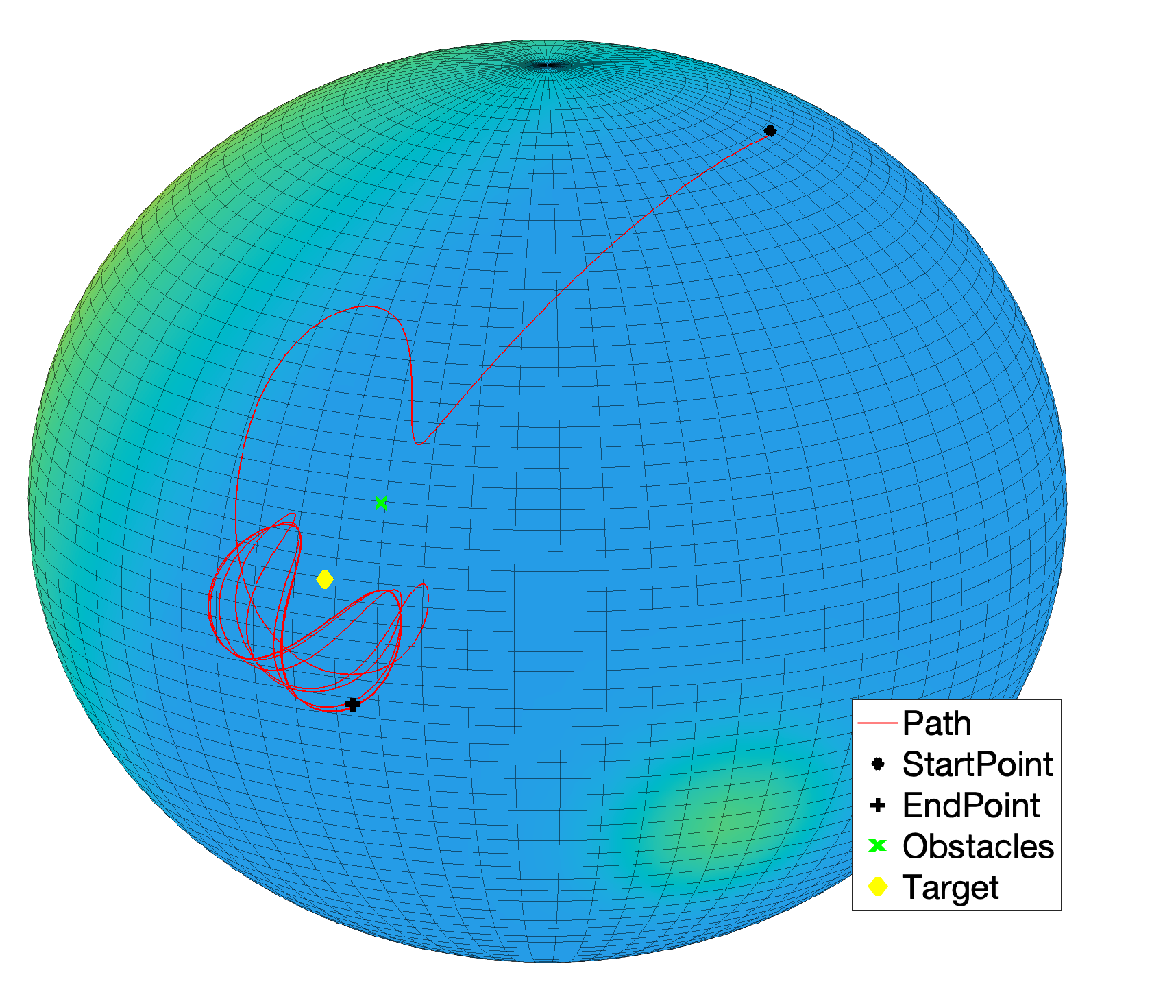
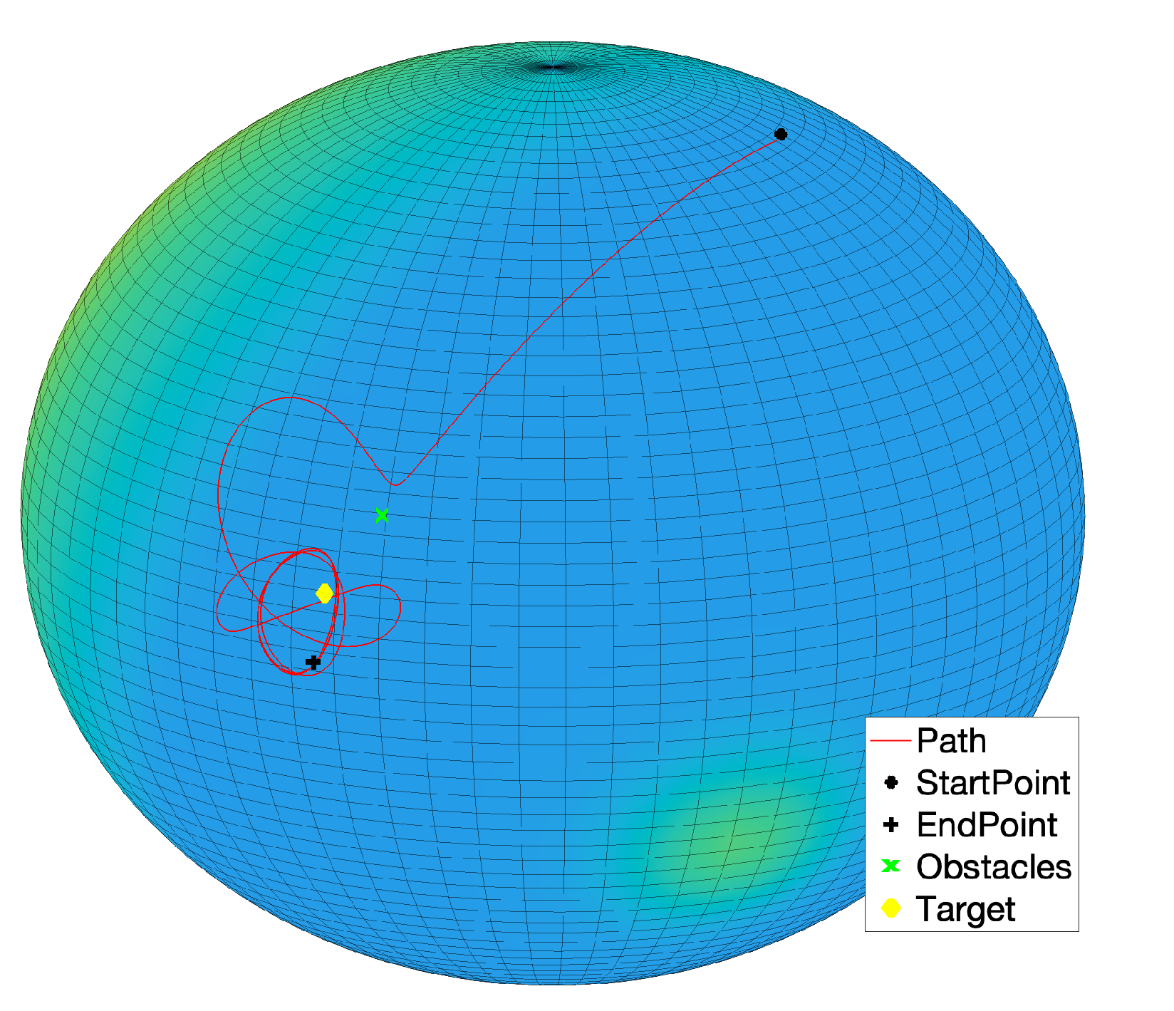
A further set of experiments were designed that include one obstacle between the start location and the target location. The state trajectory of the system looks interesting, and aligned to the corresponding behavior seen in Section 3. In fact, the state trajectory of the system at the beginning of the simulation takes the shortest path to reach the target but, when the state gets close enough to the obstacle, it gets repelled and takes a detour to reach the target. As soon as the system approaches the target, its state trajectory reveals an interesting aspect of the VARP control method: since each location in the virtual potential field (that could represent an obstacle or a target) may be associated with both an attractive and a repulsive action, the system will not turn around the target since it is repelled by both the target and the obstacle, as illustrated in Figure 17. Reducing the magnitude of the repulsive potential of the target and of the obstacle, the system state would keep go round the target as shown in Figure 18. From such simulation, we can also notice that, before being repelled, the system state comes closer to the obstacle since its repulsive action was diminished.

Setting suitable parameters values, the controlled system is able to reach the target also in the presence of two (or more) obstacles, by avoiding the virtual potential bump, as illustrated in Figure 19.

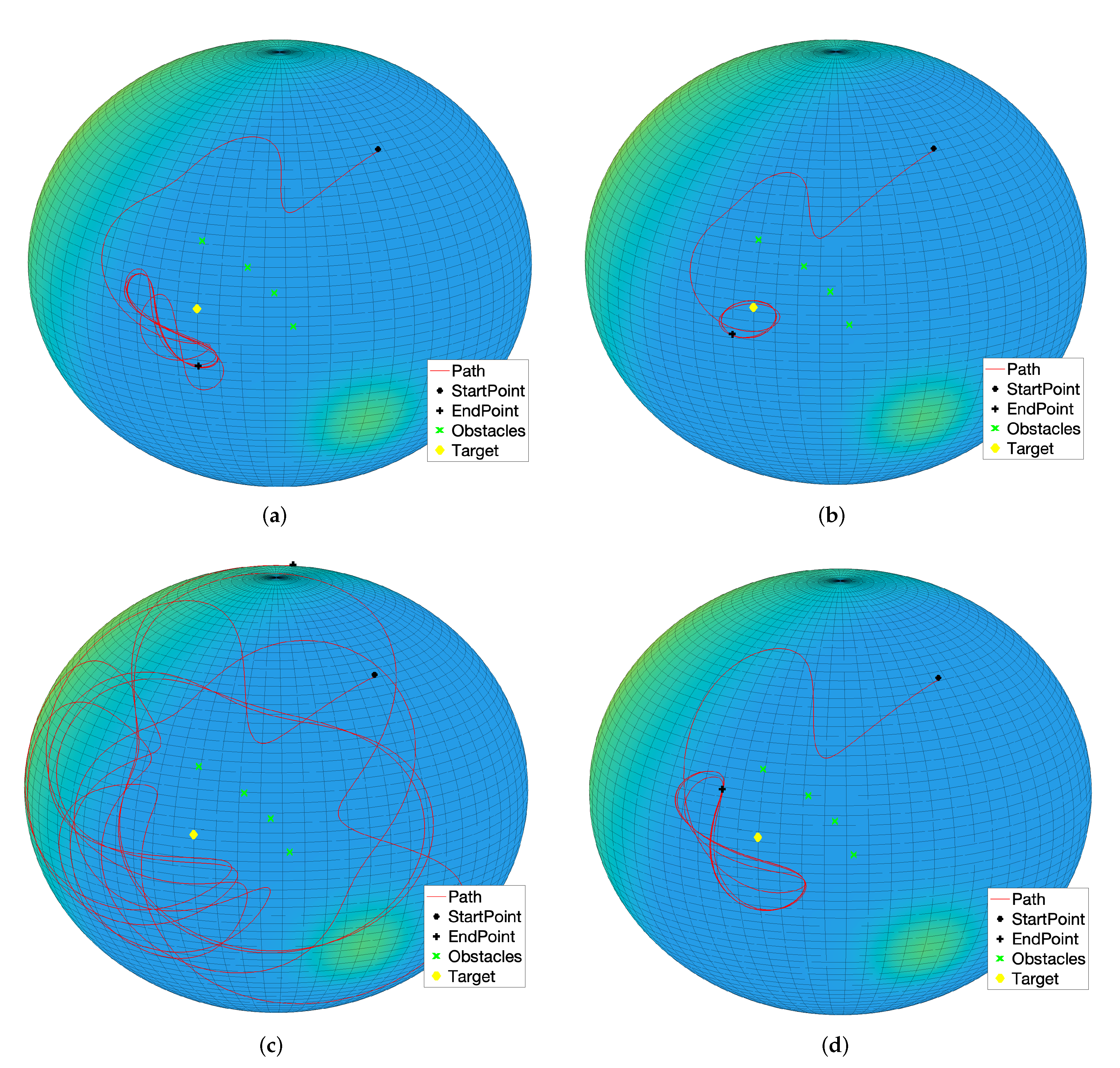
Even in the present set of experiments concerning the M-VARP control method, it is interesting to observe how the controlled system behaves when a barrier made of pointwise obstacles is placed between the starting location and the target. Figure 20a illustrates how the controlled dynamical system is able to get around a barrier in order to reach the target. From this figure it is readily appreciated how the controlled agent is unable to get close to the target since the range of influence of the obstacles and their repulsive potentials exert a strong action. By setting lower values for both the repulsive range parameter and the repulsive magnitude of the obstacles makes the controlled system get closer and turn around the target, as illustrated in Figure 20b.

By increasing both the repulsive strength of the obstacles and the self-propelling coefficient, the system will loose control and will start a rapid oscillatory behavior around the barrier and the target, as it can be observed from Figure 20c. It is interesting to notice that, despite the system propulsion induced by the self-propelling term is way stronger than necessary and the system’s state wanders all over the sphere, yet the agent will never hit the barrier. To make the trajectory smoother and bound to the target, it pays to set a higher attractive magnitude for the target in order to counteract the self-propelling term. Such a conclusion may be drawn by observing the simulation result presented in the Figure 20d.

5. Conclusions and Future Work

The VARP theory developed in [39] was originally designed to control a dynamical system whose state equations were formulated on a Euclidean space. The first part of the present contribution aimed at presenting a review of such an instance of VARP control methods as well as a comprehensive set of numerical experiments to illustrate its features in controlling a simple robot with three degrees of freedom. A limited portion of such review was devoted to recall a numerical method to simulate a controlled system as well as to implement the VARP control method on a computing platform.

Based on the understanding acquired on the VARP theory and on its numerical implementation, the second part of the present paper introduced an extension of the VARP control method to regulate the dynamics of second-order systems whose state space takes the form of Riemannian manifolds. Extensive numerical experiments conducted on the ${\mathbb{S}}^2$ manifold proved the effectiveness of the introduced M-VARP theory to control the motion of a dynamical system presenting holonomic constraints in its state-variables. Besides of the present proof-of-concept, applications of the devised theory to realistic engineering cases are currently being pursued.

From a methodological viewpoint, the encouraging results displayed within the present paper suggest a number of further investigations, which are briefly outlined in the following:

• the control method termed M-VARP has been shown effective through numerical experiments; it would be interesting to conduct a theoretical analysis (i.e., Lyapunov-like) about its effectiveness and about its applicability;
• the displayed experiments confirmed that the construction of a potential barrier represents a viable method to guide a dynamical system toward a predefined target; the notion of potential barrier might be extended by the notion of potential corridor that might afford better control of a systems’ trajectory;
• the original VARP control theory was developed to achieve cooperative control; such important feature has not been exploited in the present study, since it has been assumed the presence of a single controlled agent; nevertheless, the M-VARP theory itself inherits cooperative control ability from the VARP method; it would hence be interesting to apply the M-VARP method in a multi-agent environment;
• the M-VARP theory holds in general for Riemannian manifolds and might therefore be applied seamlessly to Lie groups; such observation implies that the devised M-VARP control theory may be applied to complex systems presenting a roto-translational dynamics, such as quadcopter drones.

Such interesting research challenges might be tackled in forthcoming endeavors.

References

- Hablani, H.B. Attitude commands avoiding bright objects and maintaining communication with ground station. J. Guid. Control. Dyn. 1999, 22, 759–767. [Google Scholar] [CrossRef]
- Wang, Z.; Mao, S.; Gong, Z.; Zhang, C.; He, J. Energy efficiency enhanced landing strategy for manned eVTOLs using L1 adaptive control. Symmetry 2021, 13, 2125. [Google Scholar] [CrossRef]
- Galyaev, A.A.; Lysenko, P.V.; Rubinovich, E.Y. Optimal stochastic control in the interception problem of a randomly tacking vehicle. Mathematics 2021, 9, 2386. [Google Scholar] [CrossRef]
- Reyes-Uquillas, D.; Hsiao, T. Compliant human–robot collaboration with accurate path-tracking ability for a robot manipulator. Appl. Sci. 2021, 11, 5914. [Google Scholar] [CrossRef]
- Connolly, C.; Grupen, R. The application of harmonic functions to robotics. J. Robot. Syst. 1993, 10, 931–946. [Google Scholar] [CrossRef] [Green Version]
- Connolly, C.I.; Burns, J.B.; Weiss, R. Path planning using Laplace’s equation. In Proceedings of the IEEE International Conference on Robotics and Automation, Sacramento, CA, USA, 13–18 May 1990; Volume 3, pp. 2102–2106. [Google Scholar]
- Chang, D.; Shadden, S.; Marsden, J.; Olfati-Saber, R. Collision Avoidance for Multiple Agent Systems. In Proceedings of the 42nd IEEE Conference on Decision and Control, Maui, HI, USA, 9–12 December 2003; pp. 539–543. [Google Scholar]
- Waydo, S.; Murray, R.M. Vehicle motion planning using stream functions. In Proceedings of the IEEE International Conference on Robotics and Automation, Taipei, Taiwan, 14–19 September 2003; Volume 2, pp. 2484–2491. [Google Scholar]
- Levine, H.; Rappel, W.J.; Cohen, I. Self-organization in systems of self-propelled particles. Phys. Rev. E 2000, 63, 017101. [Google Scholar] [CrossRef] [Green Version]
- Leonard, E.; Fiorelli, E. Virtual Leaders, Artificial Potentials and Coordinated Control of Groups. In Proceedings of the 40th IEEE Conference on Decision and Control, Orlando, FL, USA, 4–7 December 2001; pp. 2968–2973. [Google Scholar]
- Chen, Y.B.; Luo, G.C.; Mei, Y.S.; Yu, J.Q.; Su, X.L. UAV path planning using artificial potential field method updated by optimal control theory. Int. J. Syst. Sci. 2016, 47, 1407–1420. [Google Scholar] [CrossRef]
- Paul, T.; Krogstad, T.R.; Gravdahl, J.T. Modelling of UAV formation flight using 3D potential field. Simul. Model. Pract. Theory 2008, 16, 1453–1462. [Google Scholar] [CrossRef]
- Rasekhipour, Y.; Khajepour, A.; Chen, S.; Litkouhi, B. A Potential Field-Based Model Predictive Path-Planning Controller for Autonomous Road Vehicles. IEEE Trans. Intell. Transp. Syst. 2017, 18, 1255–1267. [Google Scholar] [CrossRef]
- Shimoda, S.; Kuroda, Y.; Iagnemma, K. Potential Field Navigation of High Speed Unmanned Ground Vehicles on Uneven Terrain. In Proceedings of the 2005 IEEE International Conference on Robotics and Automation, Barcelona, Spain, 18–22 April 2005; pp. 2828–2833. [Google Scholar] [CrossRef] [Green Version]
- Rimon, E.; Koditschek, D. Exact robot navigation using artificial potential functions. IEEE Trans. Robot. Autom. 1992, 8, 501–518. [Google Scholar] [CrossRef] [Green Version]
- Koditschek, D.; Rimon, E. Robot navigation functions on manifolds with boundary. Adv. Appl. Math. 1990, 11, 412–442. [Google Scholar] [CrossRef] [Green Version]
- Lee, U.; Mesbahi, M. Feedback control for spacecraft reorientation under attitude constraints via convex potentials. IEEE Trans. Aerosp. Electron. Syst. 2014, 50, 2578–2592. [Google Scholar] [CrossRef]
- McInnes, C.R. Large angle slew maneuvers with autonomous sun vector avoidance. J. Guid. Control. Dyn. 1994, 17, 875–877. [Google Scholar] [CrossRef]
- Sun, D.; Hovakimyan, N.; Jafarnejadsani, H. Design of command limiting control law using exponential potential functions. J. Guid. Control. Dyn. 2021, 44, 441–448. [Google Scholar] [CrossRef]
- Gaudet, B.; Linares, R.; Furfaro, R. Spacecraft rendezvous guidance in cluttered environments via artificial potential functions and reinforcement learning. In Proceedings of the AAS/AIAA Astrodynamics Specialist Conference, Snowbird, UT, USA, 19–23 August 2018; pp. 813–827. [Google Scholar]
- Zappulla, R.I.; Virgili-Llop, J.; Romano, M. Near-optimal real-time spacecraft guidance and control using harmonic potential functions and a modified RRT. In Proceedings of the 27th AAS/AIAA Spaceflight Mechanics Meeting, San Antonio, TX, USA, 5–9 February 2017. [Google Scholar]
- Bloise, N.; Capello, E.; Dentis, M.; Punta, E. Obstacle avoidance with potential field applied to a rendezvous maneuver. Appl. Sci. 2017, 7, 1042. [Google Scholar] [CrossRef] [Green Version]
- Zhu, S.; Yang, H.; Cui, P.; Xu, R.; Liang, Z. Anti-collision zone division based hazard avoidance guidance for asteroid landing with constant thrust. Acta Astronaut. 2022, 190, 377–387. [Google Scholar] [CrossRef]
- Cao, X.; Chen, L.; Guo, L.; Han, W. AUV Global Security Path Planning Based on a Potential Field Bio-Inspired Neural Network in Underwater Environment. Intell. Autom. Soft Comput. 2021, 27, 391–407. [Google Scholar] [CrossRef]
- Baxter, J.L.; Burke, E.K.; Garibaldi, J.M.; Norman, M. Multi-Robot Search and Rescue: A Potential Field Based Approach. In Autonomous Robots and Agents; Mukhopadhyay, S.C., Gupta, G.S., Eds.; Springer: Berlin/Heidelberg, Germany, 2007; pp. 9–16. [Google Scholar] [CrossRef]
- Huang, L. Velocity planning for a mobile robot to track a moving target—A potential field approach. Robot. Auton. Syst. 2009, 57, 55–63. [Google Scholar] [CrossRef]
- Sahu, B.; Subudhi, B. Potential function-based path-following control of an autonomous underwater vehicle in an obstacle-rich environment. Trans. Inst. Meas. Control. 2017, 39, 1236–1252. [Google Scholar] [CrossRef]
- Tamzidul, M.; Yogang, S.; Byung-Cheol, M. Maneuvering ability-based weighted potential field framework for multi-USV navigation, guidance, and control. Mar. Technol. Soc. J. 2020, 54, 40–58. [Google Scholar] [CrossRef]
- Bellini, A.; Lu, W.; Naldi, R.; Ferrari, S. Information driven path planning and control for collaborative aerial robotic sensors using artificial potential functions. In Proceedings of the 2014 American Control Conference, Portland, OR, USA, 4–6 June 2014; pp. 590–597. [Google Scholar] [CrossRef]
- Lee, M.C.; Park, M.G. Artificial potential field based path planning for mobile robots using a virtual obstacle concept. In Proceedings of the 2003 IEEE/ASME International Conference on Advanced Intelligent Mechatronics (AIM 2003), Kobe, Japan, 20–24 July 2003; Volume 2, pp. 735–740. [Google Scholar] [CrossRef]
- Choset, H.; Lynch, K.M.; Hutchinson, S.; Kantor, G.A.; Burgard, W.; Kavraki, L.E.; Thrun, S. Principles of Robot Motion—Theory, Algorithms, and Implementations; MIT Press: Boston, MA, USA, 2005. [Google Scholar]
- Kamon, I.; Rimon, E.; Rivlin, E. TangentBug: A Range-Sensor-Based Navigation Algorithm. Int. J. Robot. Res. 1998, 17, 934–953. [Google Scholar] [CrossRef]
- Kamon, I.; Rivlin, E. Sensory-Based Motion Planning with Global Proofs. IEEE Trans. Robot. Autom. 1997, 13, 814–822. [Google Scholar] [CrossRef] [Green Version]
- Lumelsky, V.; Stepanov, A. Dynamic path planning for a mobile automaton with limited information on the environment. IEEE Trans. Autom. Control. 1986, 31, 1058–1063. [Google Scholar] [CrossRef]
- Magid, E.; Rivlin, E. CautiousBug: A competitive algorithm for sensory-based robot navigation. In Proceedings of the 2004 IEEE/RSJ International Conference on Intelligent Robots and Systems (IROS) (IEEE Cat. No.04CH37566), Sendai, Japan, 28 September–2 October 2004; Volume 3, pp. 2757–2762. [Google Scholar]
- Wang, M.; Su, Z.; Tu, D.; Lu, X. A hybrid algorithm based on Artificial Potential Field and BUG for path planning of mobile robot. In Proceedings of the 2013 2nd International Conference on Measurement, Information and Control, Harbin, China, 16–18 August 2013; Volume 2, pp. 1393–1398. [Google Scholar] [CrossRef]
- Ren, J.; McIsaac, K.A.; Patel, R.V. Modified Newton’s method applied to potential field-based navigation for mobile robots. IEEE Trans. Robot. 2006, 22, 384–391. [Google Scholar] [CrossRef]
- Li, G.; Yamashita, A.; Asama, H.; Tamura, Y. An efficient improved artificial potential field based regression search method for robot path planning. In Proceedings of the 2012 IEEE International Conference on Mechatronics and Automation, Chengdu, China, 5–8 August 2012; pp. 1227–1232. [Google Scholar] [CrossRef]
- Nguyen, B.; Chuang, Y.L.; Tung, D.; Hsieh, C.; Jin, Z.; Shi, L.; Marthaler, D.; Bertozzi, A.; Murray, R. Virtual attractive-repulsive potentials for cooperative control of second order dynamic vehicles on the Caltech MVWT. In Proceedings of the 2005 American Control Conference, Portland, OR, USA, 8–10 June 2005; pp. 1084–1089. [Google Scholar]
- Fiori, S. Manifold calculus in system theory and control–Fundamentals and first-order systems. Symmetry 2021, 13, 2092. [Google Scholar] [CrossRef]
- Fiori, S.; Cervigni, I.; Ippoliti, M.; Menotta, C. Extension of a PID control theory to Lie groups applied to synchronizing satellites and drones. IET Control. Theory Appl. 2020, 14, 2628–2642. [Google Scholar] [CrossRef]
- Tarsi, A.; Fiori, S. Lie-group modeling and numerical simulation of a helicopter. Mathematics 2021, 9, 2682. [Google Scholar] [CrossRef]
- Fiori, S.; Del Rossi, L. Minimal control effort and time Lie-group synchronization design based on proportional-derivative control. Int. J. Control. 2022, 95, 138–150. [Google Scholar] [CrossRef]
Figure 1.
Schematic of Kelly robot’s geometry and of the reference systems used to model its dynamics, as well as of the thrusts acting on Kelly robot’s body as generated by the fan-type propellers.
Figure 2.
Experiment: Single target and no obstacles. Self-propelling coefficient . Friction coefficient kg/s. Target attractive magnitude and target attractive range . Simulation time s. In the 3D potentials graph, the red line represents the trajectory of the Kelly robot and the blue potential pit denotes the attractive influence of the target point: considering the Kelly robot as a rolling ball, it will ‘fall’ into the potential pit. The orientation of the Kelly robot is measured in radians (in the range ) hence, in the orientation graph, the spikes correspond to a jump from 0 to or vice versa. (a) Target approaching; (b) control figures.
Figure 3.
Experiment: Single obstacle and target. Self-propelling coefficient . Friction coefficient kg/s. Target attractive magnitude and target attractive range . Obstacle repulsive magnitude and obstacle repulsive range . Simulation time s. In the 3D potentials graph, it may be noticed a spike in the potential function surface that represents the repulsive influence of the obstacle. (a) Target approaching; (b) control figures.
Figure 4.
Experiment: Single obstacle and target. Self-propelling coefficient (i.e., five times larger than in Figure 3). Friction coefficient kg/s. Target attractive magnitude and target attractive range . Obstacle repulsive magnitude and obstacle repulsive range . Simulation time s. Even in this case, in the 3D potentials graph, it may be noticed the red line proceeding toward the bottom of the potential pit and a spike in the potential function surface that represents the obstacle.
Figure 5.
Experiment: Single obstacle and target. Self-propelling coefficient . Friction coefficient kg/s. Target attractive magnitude and target attractive range . Notice that the target attractive magnitude has an higher value compared to the simulation in Figure 4, hence the potential depression appears to be sharper. Obstacle repulsive magnitude and obstacle repulsive range . Simulation time s.
Figure 6.
Experiment: Construction of a barrier. Self-propelling coefficient . Friction coefficient kg/s. Target attractive magnitude and target attractive range . Obstacles repulsive magnitude , and obstacles repulsive ranges , , where the footers denote obstacles indexes as illustrated in the target approaching panel. Simulation time s. (a) Target approaching; (b) control figures.
Figure 7.
Experiment: Construction of a barrier. Self-propelling coefficient . Friction coefficient kg/s. Target attractive magnitude and target attractive range . Obstacles repulsive magnitude and obstacles repulsive ranges , . Simulation time s. (a) Target approaching; (b) control figures.
Figure 8.
Experiment: Construction of a barrier. Self-propelling coefficient . Friction coefficient kg/s. Target attractive magnitude and target attractive range . Obstacles repulsive magnitudes , and obstacles repulsive ranges . Simulation time s. (a) Target approaching; (b) control figures.
Figure 9.
Figure 10.
Experiment: Path planning by a guiding potential wall. Self-propelling coefficient . Friction coefficient kg/s. Target attractive magnitude and target attractive range . Obstacle repulsive magnitude and obstacle repulsive range . Simulation time s. In the 3D potentials graph, potential spikes–representing obstacles–that drive a Kelly robot towards the target point are clearly visible. (a) Target approaching; (b) control figures.
Figure 11.
Experiment: Single target, no obstacles, initial orientation . Self-propelling coefficient . Friction coefficient kg/s. Target attractive magnitude , target attractive range . Simulation time s.
Figure 12.
Experiment: Single target, no obstacles, initial orientation . Values of the parameters as in Figure 11.
Figure 13.
Figure 14.
Figure 15.
Experiment by the -VARP method: Single target, no obstacles. Simulation parameters: , , , . (a) Parameter . steps = 500; (b) parameter . steps = 500; (c) parameter , steps = 500; (d) parameter , steps = 5000.
Figure 16.
Experiment by the -VARP method: Single target, no obstacles. Simulation parameters: , . Steps = 500.
Figure 17.
Experiment by the -VARP method: Target and one obstacle. Simulation parameters: , , (where stands for Target and stands for Obstacle).
Figure 18.
Figure 19.
Experiment by the -VARP method: Target and two obstacles. Simulation parameters: , , (where stands for Target and stands for Obstacle).
Figure 20.
Experiment by the -VARP method: Potential wall (or ‘barrier’). (In the subcaptions, superscript stands for Target while superscript stands for Obstacle). (a) Parameters: , , , ; (b) parameters: , , ; (c) parameters: , , , ; (d) parameters: , , , .
Publisher’s Note: MDPI stays neutral with regard to jurisdictional claims in published maps and institutional affiliations. |
© 2022 by the authors. Licensee MDPI, Basel, Switzerland. This article is an open access article distributed under the terms and conditions of the Creative Commons Attribution (CC BY) license (https://creativecommons.org/licenses/by/4.0/).
Share and Cite
MDPI and ACS Style
Bigelli, L.; Polenta, F.; Fiori, S. Virtual Attractive-Repulsive Potentials Control Theory: A Review and an Extension to Riemannian Manifolds. Symmetry 2022, 14, 257. https://0-doi-org.brum.beds.ac.uk/10.3390/sym14020257
AMA Style
Bigelli L, Polenta F, Fiori S. Virtual Attractive-Repulsive Potentials Control Theory: A Review and an Extension to Riemannian Manifolds. Symmetry. 2022; 14(2):257. https://0-doi-org.brum.beds.ac.uk/10.3390/sym14020257
Chicago/Turabian StyleBigelli, Luca, Federico Polenta, and Simone Fiori. 2022. "Virtual Attractive-Repulsive Potentials Control Theory: A Review and an Extension to Riemannian Manifolds" Symmetry 14, no. 2: 257. https://0-doi-org.brum.beds.ac.uk/10.3390/sym14020257
Note that from the first issue of 2016, this journal uses article numbers instead of page numbers. See further details here.