Research on Comparision between Deterministic Method and Uncertain Method for Solving Uncertain Multiobjective Programming

Abstract

Since there are often few or no samples and asymmetry information in the problems, uncertainty theory is introduced to study uncertain multi-objective programming (UMP), which cannot be solved by probability theory. Generally speaking, there are two types of methods for solving the UMP problem: in deterministic method, using the numerical characteristics of an uncertain variable, the UMP problem is transformed into a deterministic multiobjective programming, and then solved by the weighting method and ideal point method; in the uncertain method, the UMP problem is transformed into an uncertain single-objective programming, and then is solved by the evaluation criteria of the uncertain variables. The theoretical analysis and the data results for numerical examples solved by the AC algorithm designed in the paper show that the two types of methods are obviously different. Further, using this comparison, the essential difference between the two methods is whether the uncertainty relation between objective functions sholud be considered. Therefore, when the uncertainty relation is closely related, the uncertain method is more appropriate; otherwise, the deterministic method should be chosen.

1. Introduction

To study decision-making problems with multiple and conflicting objectives in the real world, multiobjective programming has been widely studied by researchers in a variety of fields, especially in the field of operational research, which can be referred to in the literature [1,2,3,4,5]. It can be seen that the above literature on multiobjective programming mainly focuses on the deterministic environment. When uncertain factors are involved, many scholars regard them as random phenomena and put forward stochastic multi-objective programming (SMP). SMP is generally closer to practical problems and has been widely developed in many areas of application, which can be referred to in References [6,7,8,9,10].

Most of the above literature remains at the application level, and the adopted theoretical solution methods are relatively simple. The main method used to deal with the random factors in SMP is taking the expected value of the objective functions and then transforming the initial SMP into a determined, multi-objective programming problem; namely, the expected value model of SMP. However, in a practical decision-making problem, in addition to considering the lowest average cost, the decision scheme with the lowest fluctuation is necessary. Therefore, the expected value model of SMP is not very close to the actual problem. More problematically, a fundamental premise of employing probability theory is that the estimated probability distribution is close enough to the real frequency. Due to the non-experimental and complex nature of the practical problem, the sample size in the multiobjective programming problem is often too small to estimate the probability distribution, so the uncertainties cannot be dealt with using probability theory, especially when the information is vague. This can be seen in Reference [11], for example. Therefore, we cannot deal with multiobjective programming problems with this type of indeterminacy based on probability theory, as the final decision would not be in line with reality. In order to solve this type of indeterminacy, called uncertainty, with an expert degree of belief, this paper introduces the uncertainty theory founded by professor Liu in 2007 [12] and refined in 2010 based on normality, duality, subadditivity, and product axioms [13]. To date, a high number of studies have proved that uncertainty theory is a branch of mathematics used to model human uncertainty and has been widely used, not only in theoretical fields such as Liu [14], Wang et al. [15], Liu and Yao [16], Wen et al. [17], etc., but also in application fields such as Zheng et al. [18], Zheng et al. [19], Zhang et al. [20], and Wang et al. [21], etc. However, except for the concepts of efficient solution and the expected-value model based on uncertain variables mentioned in the literatures [14,22], the research on uncertain multi-objective programming (UMP) based on uncertain theory is not in-depth enough.

In view of the disadvantages of the above research, based on uncertainty theory, this paper carries out research into the solution methods of the UMP problem, which are defined as deterministic method and uncertain method, respectively. To date, there are few relevant results on the comparison of these two types of solution method, and only two pieces of relevant literature have been found in the stochastic environment, by Caballero [23] and Gutjahr [24]. In the literature [23], based on the expected value criterion of random variables, Caballero only uses the linear weighting method to compare these two types of solution methods for stochastic multiobjective programming. In this case, it was concluded that the efficient solutions were exactly the same, but in other criteria, such as minimum variance criterion, maximum probability criteria, etc., they were different. In the literature [24], Gutjahr only mentions the ideas of these two solution methods, and does not carry out detailed and specific research contents. However, in the environment of uncertainty with an expert’s degree of belief, there are few research results on the two types of solution to the UMP problem, based on uncertainty theory. Further, unlike random variables, the expected values of uncertain variables do not have linear properties; thus, except for cases where uncertain variables are independent of each other or comonotonic, even with the expected value criterion and the linear weighting method used, the efficient solutions obtained by the two types of solution method are different. This differs from the results obtained in the literature [23]. In addition, based on the ideal point method, the efficient solutions obtained in these two types of solution method are completely different whether used in a stochastic environment or uncertainty environment with expert’s degree of belief. The mainly innovative research contents proposed in this paper are as follows:

(a) Research on the deterministic method. Firstly, the UMP model with uncertain vectors in the objective functions is presented. Based on the expected value of the uncertain vector, the expected value model of the UMP (E-UMP) problem is proposed. Secondly, since the E-UMP problem only considers the minimum average cost of the uncertain objective functions, in the practical problem, it often needs to take consider the minimum fluctuation. Therefore, in order to consider the fluctuation in the practical problem, the expected-value variance model of the UMP (EV-UMP) problem is proposed, taking both expectation and variance for the uncertain objective functions. Whether the E-UMP model or the EV-UMP model is used, their common point is to transform the initial UMP problem into a deterministic multi-objective programming problem. Therefore, this type of solution method is called a deterministic method. Finally, the E-UMP model and EV-UMP model are transformed into the determined single-objective programming (DSP) problems by the weighting method and ideal point method proposed in this paper, and it is proved that the optimal solutions to the DSP problems are the expected-value efficient solutions to the initial UMP problem.

(b) Research into the uncertain method. It is easy to see that the deterministic method first transforms the uncertain multi-objective functions in the UMP problem into the deterministic multi-objective functions, so the uncertainty relation between them is separated and also disappeared. When the uncertainties between uncertain objective functions are closely related, the deterministic method is infeasible. To overcome this disadvantage, we first transform the initial UMP problem into an uncertain single-objective programming (USP) problem by introducing a measurable function, G, which remains the uncertainty relation between uncertain objective functions. This type of solution method is called the uncertain method. Then, in order to provide the optimal solution concept to the USP problem, we define the order relationship between the uncertain variables based on different evaluation criterions. Since the average value is frequently used in real-world problems, the $C_E$ evaluation criterion is employed throughout this paper. Based on the $C_E$ evaluation criteria and the measurable function G constructed by the linear weighted construction method and ideal point construction method, $C_E$-optimal solutions to the USP problem can be obtained. Finally, we prove that the $C_E$-optimal solutions to the USP problem are the $C_E$-efficient solutions to the initial UMP problem under the $C_E$ evaluation criterion.

(c) Comparison of two types of solution method. On the one hand, from theoretical analysis, we can see that the deterministic method first uses their expectation of the objective functions in the UMP problem, and then transforms it into a single-objective programming, while the uncertain method does the opposite. Generally speaking, for the uncertain variable, we have

$$G\left(E\left[f_1(x,{\xi }_1)\right],\cdots ,E\left[f_s(x,{\xi }_s)\right]\right)\ne E\left[G\left(f_1(x,{\xi }_1),\cdots ,f_s(x,{\xi }_s)\right)\right],$$

where $G(·)$ is a measurable function. Therefore, the theoretical results for these two types of method are different. On the other hand, according to the solution results of the numerical examples illustrated in this paper, the efficient solutions obtained by the two types of solution methods are also different.

The paper is organized as follows. Some basic results of uncertainty theory are reviewed in the next section. In Section 3, based on uncertainty theory, the UMP model is proposed. In Section 4, the deterministic method is studied, and a numerical example is provided to illustrate the solution method. In Section 5, the uncertain method is proposed when the uncertainties between uncertain objective functions are closely related, and a numerical example is also given to illustrate the uncertain method. Furthermore, the two types of solution methods are compared and analyzed according to the data results of the numerical examples. Finally, a brief summary is given in Section 6.

2. Theoretical Background

Let $\Gamma$ be a nonempty set, and $\mathcal{L}$ a $\sigma$-algebra over $\Gamma$. Each element $\Lambda$ in $\mathcal{L}$ is called an event. A set function $\mathcal{M}$ from $\mathcal{L}$ to $[0,1]$ is called an uncertain measure if it satisfies the following axioms [12]:

Axiom 1.

(Normality Axiom) $\mathcal{M}\{\Gamma \}=1$ for the universal set $\Gamma$.

Axiom 2.

(Duality Axiom) $\mathcal{M}\{\Lambda \}+\mathcal{M}\left\{{\Lambda }^c\right\}=1$ for any event $\Lambda$.

Axiom 3.

(Subadditivity Axiom) For every countable sequence of events ${\Lambda }_1,{\Lambda }_2,\cdots$, we have

$$\mathcal{M}\left\{\bigcup _{i=1}^{\infty }{\Lambda }_i\right\}\le \sum _{i=1}^{\infty }\mathcal{M}\left\{{\Lambda }_i\right\}.$$

(1)

The triplet $(\Gamma ,\mathcal{L},\mathcal{M})$ is called an uncertainty space. Furthermore, Liu [25] defined a product of uncertain measure by the fourth axiom:

Axiom 4.

(Product Axiom) Let $({\Gamma }_k,{\mathcal{L}}_k,{\mathcal{M}}_k)$ be an uncertainty space for $k=1,2,\cdots$. The product of uncertain measure $\mathcal{M}$ is an uncertain measure satisfying

$$\mathcal{M}\left\{\prod _{k=1}^{\infty }{\Lambda }_k\right\}={\displaystyle \underset{k=1}{\overset{\infty }{\bigwedge }}}{\mathcal{M}}_k\left\{{\Lambda }_k\right\}$$

(2)

where ${\Lambda }_k$ are arbitrarily chosen events from ${\mathcal{L}}_k$ for $k=1,2,\cdots$, respectively.

Roughly speaking, an uncertain variable is a measurable function on an uncertainty space. A formal definition is given as follows.

Definition 1.

[12] An uncertain variable is a measurable function ξ from an uncertainty space $(\Gamma ,\mathcal{L},\mathcal{M})$ to the set of real numbers, i.e., for any Borel set B of real numbers, the set

$$\{\xi \in B\}=\{\gamma \in \Gamma \mid \xi (\gamma )\in B\}$$

(3)

is an event.

Definition 2.

[12] The uncertainty distribution$\Phi$of an uncertain variable ξ is defined by $\Phi \left(x\right)=\mathcal{M}\{\xi \le x\}$ for any real number x.

Definition 3.

[25] The uncertain variables ${\xi }_1,{\xi }_2,\cdots ,{\xi }_n$ are said to be independent if

$$\mathcal{M}\left\{\bigcap _{i=1}^n\left({\xi }_i\in B_i\right)\right\}=\underset{i=1}{\overset{n}{\bigwedge }}\mathcal{M}\{{\xi }_i\in B_i\}$$

(4)

for any Borel sets $B_1,B_2,\dots ,B_n$ of real numbers.

Theorem 1.

[13] Let ${\xi }_1,{\xi }_2,\cdots ,{\xi }_n$ be uncertain variables, and f a real-valued measurable function. Then, $f({\xi }_1,{\xi }_2,\cdots ,{\xi }_n)$ is an uncertain variable.

Theorem 2.

[13] Let ${\xi }_1,{\xi }_2,\cdots ,{\xi }_n$ be independent uncertain variables with continuous uncertainty distributions ${\Phi }_1,{\Phi }_2,\cdots ,{\Phi }_n$, respectively. If f is a strictly increasing function, then the uncertain variable

$$\xi =f({\xi }_1,{\xi }_2,\cdots ,{\xi }_n)$$

(5)

has an uncertainty distribution

$$\Psi \left(x\right)=\underset{f(x_1,x_2,\cdots ,x_n)=x}{sup}\underset{1\le i\le n}{min}{\Phi }_i\left(x_i\right).$$

(6)

Definition 4.

[12] Let ξ be an uncertain variable. Then, the expected value of ξ is defined by

$$\mathrm{E}\left[\xi \right]={\int }_0^{\infty }\mathcal{M}\{\xi \ge x\}dx-{\int }_{-\infty }^0\mathcal{M}\{\xi \le x\}dx$$

(7)

provided that at least one of the two integrals is finite.

Theorem 3.

[13] Let ${\xi }_1,{\xi }_2,\cdots ,{\xi }_n$ be independent uncertain variables with regular uncertainty distributions ${\Phi }_1,{\Phi }_2,\cdots ,{\Phi }_n$, respectively. If the function $f(x_1,x_2,\cdots ,x_n)$ is strictly increasing with respect to $x_1,x_2,\cdots ,x_m$ and strictly decreasing with respect to $x_{m+1},x_{m+2},\cdots ,x_n$, then $\xi =f({\xi }_1,{\xi }_2,\cdots ,{\xi }_n)$ is an uncertain variable with inverse uncertainty distribution

$$\begin{array}{c}{\Psi }^{-1}\left(\alpha \right)=f\left({\Phi }_1^{-1}\left(\alpha \right),\cdots ,{\Phi }_m^{-1}\left(\alpha \right),{\Phi }_{m+1}^{-1}(1-\alpha ),\cdots ,{\Phi }_n^{-1}(1-\alpha )\right).\hfill \end{array}$$

(8)

Definition 5.

[26] When the distribution function of the uncertain variable ξ has the following linear uncertainty distribution,

$$\Phi \left(x\right)=\left\{\begin{array}{cc}0,& x\le a\\ \frac{x-a}{b-a},& a\le x\le b\\ 1,& x\ge b,\end{array}\right.$$

(9)

then ξ is called a linear uncertain variable, denoted as $\xi \sim \mathcal{L}(a,b)$, where a and b are all real numbers and $a<b$.

Definition 6.

[26] When the distribution function of the uncertain variable ξ has the following zigzag uncertainty distribution,

$$\Phi \left(x\right)=\left\{\begin{array}{cc}0,& x\le a\\ \frac{(x-a)}{2(b-a)},& a\le x\le b\\ \frac{x+c-2b}{2(c-b)},& b\le x\le c\\ 1,& x\ge c,\end{array}\right.$$

(10)

then ξ is a zigzag uncertain variable, denoted as $\xi \sim \mathcal{Z}(a,b,c)$, where a, b and c are all real numbers and $a<b<c$.

Definition 7.

[26] When the distribution function of the uncertain variable ξ has the following normal uncertainty distribution,

$$\Psi \left(x\right)={\left(1+exp\left(\frac{\pi \left(e-x\right)}{\sqrt{3}\sigma }\right)\right)}^{-1},x\in R$$

(11)

then ξ is called a normal uncertain variable, denoted as $\xi \sim \mathcal{N}(e,\sigma )$.

It is clear that a regular uncertainty distribution $\Phi \left(x\right)$ has an inverse function on the range of x, with $0<\Phi \left(x\right)<1$, and the inverse function ${\Phi }^{-1}\left(x\right)$ exists on the open interval $\left(0,1\right)$.

Definition 8.

[13] Let ξ be an uncertain variable with regular uncertainty distribution $\Phi$. Then, the inverse function ${\Phi }^{-1}$ is called the inverse uncertainty distribution of ξ.

Theorem 4.

[13] Let ξ be an uncertain variable with regular uncertainty distribution $\Phi$. If the expected value exists, then

$$\mathrm{E}\left[\xi \right]={\int }_0^1{\Phi }^{-1}\left(\alpha \right)d\alpha .$$

(12)

Theorem 5.

[27] Let ${\xi }_1,{\xi }_2,\cdots ,{\xi }_n$ be independent uncertain variables with regular uncertainty distributions ${\Phi }_1,{\Phi }_2,\cdots ,{\Phi }_n$, respectively. If the function $f(x_1,x_2,\cdots ,x_n)$ is strictly increasing with respect to $x_1,x_2,\cdots ,x_m$ and strictly decreasing with respect to $x_{m+1},x_{m+2},\cdots ,x_n$, then the uncertain variable $\xi =f({\xi }_1,{\xi }_2,\cdots ,{\xi }_n)$ has an expected value

$$\begin{array}{c}{\displaystyle E\left[\xi \right]={\int }_0^{1}f\left({\Phi }_1^{-1}\left(\alpha \right),\cdots ,{\Phi }_m^{-1}\left(\alpha \right),{\Phi }_{m+1}^{-1}(1-\alpha ),\cdots ,{\Phi }_n^{-1}(1-\alpha )\right)d\alpha .}\hfill \end{array}$$

(13)

Theorem 6.

[13] Let ξ and η be independent uncertain variables with finite expected values. Then, for any real numbers a and b, we have

$$\mathrm{E}[a\xi +b\eta ]=a\mathrm{E}\left[\xi \right]+b\mathrm{E}\left[\eta \right].$$

(14)

Theorem 7.

[22] Let f and g be comonotonic functions. Then, for any uncertain variable ξ, we have

$$\mathrm{E}\left[f\right(\xi )+g(\xi \left)\right]=\mathrm{E}\left[f\right(\xi \left)\right]+\mathrm{E}\left[g\right(\xi \left)\right].$$

(15)

Theorem 8.

[14] Let ξ be an uncertain variable with regular uncertainty distribution $\Phi$ and finite expected value e. Then,

$$V\left[\xi \right]={\int }_0^1{({\Phi }^{-1}\left(\alpha \right)-e)}^{2}d\alpha .$$

(16)

Theorem 9.

[26] If ξ is an uncertain variable with finite expected value, a and b are real numbers; then,

$$V[a\xi +b]=a^{2}V\left[\xi \right].$$

(17)

3. Uncertain Multiobjective Programming Model

Based on uncertainty theory, this section focuses on multiobjective programming with uncertain vectors, which is called the uncertain multiobjective programming (UMP) problem. Since the uncertainties in the objective functions are treated in the same way as those under constraint conditions, without loss of generality, we assume that only the objective functions in the UMP model involve the uncertain vector. Let $f_i(x,{\mathbf{\xi }}_i)$, $i=1,2,\cdots ,s$, be the objective function with uncertain variables, and S be the deterministic feasible set; then, the UMP model can be established as follows:

$$\left(\mathrm{UMP}\right)\left\{\begin{array}{cc}\underset{x\in R}{min}\hfill & \left(f_1(x,{\mathbf{\xi }}_1),f_2(x,{\mathbf{\xi }}_2),\cdots ,f_s(x,{\mathbf{\xi }}_s)\right)\hfill \\ \mathrm{s}.\mathrm{t}.\hfill & x\in S\hfill \end{array}\right.$$

(18)

where $x=(x_1,x_2,\cdots ,x_n)\in R^n$ is a decision-making variable; ${\mathbf{\xi }}_i$, $i=1,2,\cdots ,s$ are uncertain variables.

In the UMP problem (18), assume that $f_i(x,{\mathbf{\xi }}_i)$, $i=1,2,\cdots ,s$, is a Borel measure function with respect to x. According to the definition of uncertain vector, we know that $f_i(x,{\mathbf{\xi }}_i)$ is also an uncertain variable.

For convenience, denote

$$\mathit{F}(x,\mathbf{\xi })=\left(f_1(x,{\mathbf{\xi }}_1),f_2(x,{\mathbf{\xi }}_2),\cdots ,f_s(x,{\mathbf{\xi }}_s)\right),$$

(19)

Then, the UMP problem (18) can be rewritten as the following vector minimum problem

$$\left(\mathrm{UMP}\right)\begin{array}{cc}\underset{x\in S}{min}\hfill & \mathit{F}(x,\mathbf{\xi })=\left(f_1(x,{\mathbf{\xi }}_1),f_2(x,{\mathbf{\xi }}_2),\cdots ,f_s(x,{\mathbf{\xi }}_s)\right)\hfill \end{array}$$

(20)

The key to solving the UMP problem (20) is dealing with the related uncertain variables. Next, we will give two types of solution methods, i.e., the deterministic method and uncertain method.

4. Deterministic Method for Solving Uncertain Multiobjective Programming

To deal with the uncertain variables in UMP problem (20), the most commonly used method is to transform it into a deterministic multi-objective programming problem through numerical characteristics of an uncertain variable, and then it can be solved. This method is called deterministic method. Therefore, according to the definition of uncertain variables, the following expected value model of the UMP problem (E-UMP model) can be obtained by looking at the expectation of all objective functions in the UMP problem (20):

$$(\mathrm{E}-\mathrm{UMP})\begin{array}{cc}\underset{x\in S}{min}\hfill & E\left[\mathit{F}(x,\mathbf{\xi })\right]=\left(E\left[f_1(x,{\mathbf{\xi }}_1)\right],E\left[f_2(x,{\mathbf{\xi }}_2)\right],\cdots ,E\left[f_s(x,{\mathbf{\xi }}_s)\right]\right)\hfill \end{array}$$

(21)

where $E[·]$ represents the expected value operator.

Under certain conditions, the following theorem shows that the E-UMP problem (21) is a convex programming.

Theorem 10.

Let ${\xi }_i$, $i=1,2,\cdots ,s$, degenerate into the uncertain variable, and $\mathit{F}(x,\xi )$ be continuous vector function. If the feasible set S is a covext set, $\mathit{F}(x,\xi )$ is a convex vector function on x, $\mathit{F}(x_1,{\xi }_i)$ and $\mathit{F}(x_2,{\xi }_i)$ are comonotonic on ${\xi }_i$ for any given $x_1,x_2\in S$, then the E-UMP problem (21) is a convex programming.

Proof. 

Since the feasible set S is a convex set, according to the definition of convex programming, we need to prove that the objective function $E\left[\mathit{F}\right(x,\mathbf{\xi }\left)\right]$ is a convex function. Since $\mathit{F}(x,\xi )$ is a convex vector function, we can obtain

$$\mathit{F}(\alpha x_1+(1-\alpha )x_2,{\xi }_i)\le \alpha \mathit{F}(x_1,{\xi }_i)+(1-\alpha )\mathit{F}(x_2,{\xi }_i),$$

(22)

for any $\alpha \in (0,1)$ and $x_1,x_2\in S$.

Since the $\mathit{F}(x_1,{\xi }_i)$ and $\mathit{F}(x_2,{\xi }_i)$ are comonotonic on ${\xi }_i$, according to Theorem 7, the expected-value operator of an uncertain variable has the linear property; thus, the following inequality can be obtained

$$E\left[\mathit{F}(\alpha x_1+(1-\alpha )x_2,{\xi }_i)\right]\le \alpha E\left[\mathit{F}(x_1,{\xi }_i)\right]+(1-\alpha )E\left[\mathit{F}(x_2,{\xi }_i)\right],$$

(23)

which shows that $E\left[\mathit{F}\right(x,\mathbf{\xi }\left)\right]$ is a convex function. The theorem is proved.  □

The E-UMP problem (21) only considers the minimum average cost of the uncertain objective functions; however, in practical problems, the minimum fluctuation also should be taken into account. Therefore, the expected value of and variance in the objective functions in the UMP problem (20) are taken simultaneously, and the following expected-value variance model of the UMP (EV-UMP) problem (24) is proposed in this paper

$$(\mathrm{EV}-\mathrm{UMP})\left\{\begin{array}{cc}\underset{x}{min}\hfill & \left(E\left[\mathit{F}\right(x,\mathbf{\xi }\left)\right],V\left[\mathit{F}\right(x,\mathbf{\xi }\left)\right]\right)\hfill \\ \hfill & =(E\left[f_1(x,{\mathbf{\xi }}_1)\right],E\left[f_2(x,{\mathbf{\xi }}_2)\right],\cdots ,E\left[f_s(x,{\mathbf{\xi }}_s)\right],\hfill \\ \hfill & V\left[f_1(x,{\mathbf{\xi }}_1)\right],V\left[f_2(x,{\mathbf{\xi }}_2)\right],\cdots ,V\left[f_s(x,{\mathbf{\xi }}_s)\right])\hfill \\ \mathrm{s}.\mathrm{t}.\hfill & x\in S\hfill \end{array}\right.$$

(24)

where $E[·]$ and $V[·]$ represent the expected value operator and variance operator, respectively.

According to the numerical characteristics of uncertain vectors, it is easy to see that the E-UMP problem (21) and EV-UMP problem (24) are deterministic multiobjective programming models derived from the initial UMP problem (20). To illustrate the relationship between the efficient solutions of these two deterministic models and the efficient solutions of the initial UMP problem (20), some definitions are defined, as follows.

Definition 9.

(E-Efficiency) We say that the feasible solution $x^{*}\in S$ is an expected-value efficient solution to the UMP problem (20) if it is a Pareto efficient solution to the E-UMP problem (21), that is, there is no $x\in S$, such that

$$E\left[\mathit{F}(x,\mathbf{\xi })\right]\le E\left[\mathit{F}(x^{*},\mathbf{\xi })\right],$$

(25)

namely,

$$E\left[f_i(x,{\mathbf{\xi }}_i)\right]\le E\left[f_i(x^{*},{\mathbf{\xi }}_i)\right],i=1,2,\cdots ,s,$$

(26)

and

$$E\left[f_{i_0}(x,{\mathbf{\xi }}_{i_0})\right]<E\left[f_{i_0}(x^{*},{\mathbf{\xi }}_{i_0})\right]$$

(27)

for at least one $i_0$, $1\le i_0\le s$.

Denote the E-efficiency set to UMP problem (21) as $S_E$.

Definition 10.

(Weak E-Efficiency) We say that the feasible solution $x^{*}\in S$ is an expected-value weak efficient solution to the UMP problem (20) if it is a Pareto weak efficient solution to the E-UMP problem (21), that is, there is no $x\in S$, such that

$$E\left[\mathit{F}(x,\mathbf{\xi })\right]<E\left[\mathit{F}(x^{*},\mathbf{\xi })\right].$$

(28)

Denote the weak E-efficiency set to UMP problem (2) as $S_{WE}$.

Definition 11.

($EV$-Efficiency) We say that the feasible solution $x^{*}\in S$ is an expected-value variance efficient solution to the UMP problem (20) if it is a Pareto efficient solution to the EV-UMP problem (24), that is, there is no $x\in S$, such that

$$E\left[\mathit{F}(x,\mathbf{\xi })\right]\le E\left[\mathit{F}(x^{*},\mathbf{\xi })\right],V\left[\mathit{F}(x,\mathbf{\xi })\right]\le V\left[\mathit{F}(x^{*},\mathbf{\xi })\right],$$

(29)

namely,

$$E\left[f_i(x,{\mathbf{\xi }}_i)\right]\le E\left[f_i(x^{*},{\mathbf{\xi }}_i)\right],V\left[f_i(x,{\mathbf{\xi }}_i)\right]\le V\left[f_i(x^{*},{\mathbf{\xi }}_i)\right],i=1,2,\cdots ,s,$$

(30)

and

$$E\left[f_{i_0}(x,{\mathbf{\xi }}_{i_0})\right]<E\left[f_{i_0}(x^{*},{\mathbf{\xi }}_{i_0})\right],V\left[f_{i_0}(x,{\mathbf{\xi }}_{i_0})\right]<V\left[f_{i_0}(x^{*},{\mathbf{\xi }}_{i_0})\right]$$

(31)

for at least one $i_0$, $1\le i_0\le s$.

Denote the $EV$-efficiency set to UMP problem (20) as $S_{EV}$.

Definition 12.

(Weak $EV$-Efficiency) We say the feasible solution $x^{*}\in S$ is an expected-value variance efficient solution to the UMP problem (20) if it is a Pareto efficient solution to the EV-UMP problem (24), that is, there is no $x\in S$, such that

$$E\left[\mathit{F}(x,\mathbf{\xi })\right]<E\left[\mathit{F}(x^{*},\mathbf{\xi })\right],V\left[\mathit{F}(x,\mathbf{\xi })\right]<V\left[\mathit{F}(x^{*},\mathbf{\xi })\right].$$

(32)

Denote the weak $EV$-efficiency set to the UMP problem (20) as $S_{WEV}$.

It is easy to obtain the following relations between the efficiency sets defined above.

Theorem 11.

If $V\left[\mathit{F}\right(x,\mathbf{\xi }\left)\right]>\mathbf{0},$ then

(1) $S_E\subset S_{WE}$;

(2) $S_{EV}\subset S_{WEV}$.

Proof. 

According to the corresponding definitions, the two conclusions can easily be obtained. This theorem is proved.  □

The first step of the deterministic method is to deal with the uncertainty factors in the UMP problem through the numerical characteristics of the uncertain variables; then, the deterministic multi-objective programming problem is obtained, i.e., E-UMP or EV-UMP models. The second step is to transform the E-UMP or EV-UMP model into a deterministic single-objective programming. The weighting method and ideal-point method, which are common conversion methods, are given as follows.

4.1. Weighting Method

By assigning corresponding weights to the objective functions in the E-UMP problem (21) or EV-UMP problem (24), the following deterministic single-objective programming (DSP) models

$$\left(DS{P}_E^{\left(wm\right)}\right)\left\{\begin{array}{cc}\underset{x}{min}\hfill & f_E^{\left(wm\right)}\left(x\right)={\displaystyle \sum _{i=1}^s}{\omega }_{i}E\left[f_i(x,{\mathbf{\xi }}_i)\right]\hfill \\ \mathrm{s}.\mathrm{t}.\hfill & {\displaystyle \sum _{i=1}^s}{\omega }_i=1,{\omega }_i>0,i=1,\cdots ,s\hfill \\ \hfill & x\in S\hfill \end{array}\right.$$

(33)

and

$$\left(DS{P}_{EV}^{\left(wm\right)}\right)\left\{\begin{array}{cc}\underset{x}{min}\hfill & f_{EV}^{\left(wm\right)}\left(x\right)={\displaystyle \sum _{i=1}^s}{\omega }_i^{\left(e\right)}E\left[f_i(x,{\mathbf{\xi }}_i)\right]+{\displaystyle \sum _{i=1}^s}{\omega }_i^{\left(v\right)}V\left[f_i(x,{\mathbf{\xi }}_i)\right]\hfill \\ \mathrm{s}.\mathrm{t}.\hfill & {\displaystyle \sum _{i=1}^s}{\omega }_i^{\left(e\right)}+{\omega }_i^{\left(v\right)}=1,{\omega }_i^{\left(e\right)}>0,{\omega }_i^{\left(v\right)}>0,i=1,\cdots ,s\hfill \\ \hfill & x\in S\hfill \end{array}\right.$$

(34)

are obtained, respectively, where ${\omega }_i$, ${\omega }_i^{\left(e\right)}$ and ${\omega }_i^{\left(v\right)}$ represent their corresponding weights.

The sets of optimal solutions for model (33) and model (34) are denoted as $S_{s_e}^{\left(wm\right)}$ and $S_{s_{ev}}^{\left(wm\right)}$, respectively.

Next, we prove that the optimal solution of the $DS{P}_E^{\left(wm\right)}$ problem (33) is the expected-value efficient solution to the initial UMP model (20), and that of the $DS{P}_{EV}^{\left(wm\right)}$ problem (34) is the expected-value variance efficient solution to the initial UMP model (20).

Theorem 12.

If $V\left[\mathit{F}\right(x,\mathbf{\xi }\left)\right]>\mathbf{0},$, then:

(1) $S_{s_e}^{\left(wm\right)}\subset S_E$;

(2) $S_{s_{ev}}^{\left(wm\right)}\subset S_{EV}$.

Proof. 

It is easy to see that the proof of conclusion (18) is similar to that of conclusion (20). Without any losses of generality, only conclusion (20) needs to be proved. We prove conclusion (20) by contradiction. Suppose that $x^{*}\in S_{s_{ev}}^{\left(wm\right)}$, but $x^{*}\notin S_{EV}$. According to Definition 11, there must be at least one $\overline{x}\in S$, such that

$$E\left[\mathit{F}(\overline{x},\mathbf{\xi })\right]\le E\left[\mathit{F}(x^{*},\mathbf{\xi })\right],V\left[\mathit{F}(\overline{x},\mathbf{\xi })\right]\le V\left[\mathit{F}(x^{*},\mathbf{\xi })\right],$$

(35)

namely,

$$E\left[f_i(\overline{x},{\mathbf{\xi }}_i)\right]\le E\left[f_i(x^{*},{\mathbf{\xi }}_i)\right],V\left[f_i(\overline{x},{\mathbf{\xi }}_i)\right]\le V\left[f_i(x^{*},{\mathbf{\xi }}_i)\right],i=1,2,\cdots ,s,$$

(36)

and

$$E\left[f_{i_0}(\overline{x},{\mathbf{\xi }}_{i_0})\right]<E\left[f_{i_0}(x^{*},{\mathbf{\xi }}_{i_0})\right],V\left[f_{i_0}(\overline{x},{\mathbf{\xi }}_{i_0})\right]<V\left[f_{i_0}(x^{*},{\mathbf{\xi }}_{i_0})\right]$$

(37)

for at least one $i_0$, $1\le i_0\le s$.

Since inequality (37) holds for at least one $i_0$, and ${\omega }_i^{\left(e\right)}>0,{\omega }_i^{\left(v\right)}>0,i=1,2,\cdots ,s$, the following conclusion can be obtained by multiplying inequality (36) according to their corresponding weights and then adding

$$\begin{array}{c}\hfill \sum _{i=1}^s{\omega }_i^{\left(e\right)}E\left[f_i(\overline{x},{\mathbf{\xi }}_i)\right]+\sum _{i=1}^s{\omega }_i^{\left(v\right)}V\left[f_i(\overline{x},{\mathbf{\xi }}_i)\right]\\ \hfill <\sum _{i=1}^s{\omega }_i^{\left(e\right)}E\left[f_i(x^{*},{\mathbf{\xi }}_i)\right]+\sum _{i=1}^s{\omega }_i^{\left(v\right)}V\left[f_i(x^{*},{\mathbf{\xi }}_i)\right]\end{array}$$

(38)

namely,

$$f_{EV}^{\left(wm\right)}\left(\overline{x}\right)<f_{EV}^{\left(wm\right)}\left(x^{*}\right)$$

(39)

which is contradictory to $x^{*}\in S_{s_{ev}}^{\left(wm\right)}$, thus, $x^{*}\in S_{EV}$; that is, $S_{s_{ev}}\subset S_{EV}$. The theorem is complete.  □

4.2. Ideal Point Method

In practical decision-making problems, it is assumed that the objective functions in E-UMP problem (21) or EV-UMP problem (24) have ideal values; then, the best decision-making scheme is to make all the objective functions meet the corresponding ideal values. However, since the objective functions in the E-UMP problem (21) or EV-UMP problem (24) are usually conflicting and contradictory, a best decision-making scheme often does not exist. Hence, the next best thing is to find the sub-optimal decision-making scheme that makes the objective functions match their ideal objective values as closely as possible. This is the so-called ideal point method.

Assume that the corresponding ideal values of $E\left[f_i(x,{\mathbf{\xi }}_i)\right]$ and $V\left[f_i(x,{\mathbf{\xi }}_i)\right]$ are $f_i^{\left(e_0\right)}$ and $f_i^{\left(v_0\right)}$, $i=1,2,\cdots ,s$, respectively. Strictly speaking, the ideal objective value $f_i^{\left(e_0\right)}$ and $f_i^{\left(v_0\right)}$ can be obtained by solving the single-objective programming $\underset{x}{min}E\left[f_i(x,{\mathbf{\xi }}_i)\right]$ or $\underset{x}{min}V\left[f_i(x,{\mathbf{\xi }}_i)\right]$. Therefore, the ideal objective values $f_i^{\left(e_0\right)}$ and $f_i^{\left(v_0\right)}$ should generally satisfy the following inequalities as far as possible.

$$f_i^{\left(e_0\right)}\le \underset{x}{min}E\left[f_i(x,{\mathbf{\xi }}_i)\right],f_i^{\left(v_0\right)}\le \underset{x}{min}V\left[f_i(x,{\mathbf{\xi }}_i)\right],i=1,2,\cdots ,s.$$

(40)

According to the idea of the ideal-point method proposed above, the E-UMP problem (21) and EV-UMP problem (24) can be transformed into the following deterministic single-objective programming:

$$\left(DS{P}_E^{\left(ipm\right)}\right)\left\{\begin{array}{cc}\underset{x}{min}\hfill & {\mathit{f}}_E^{\left(ipm\right)}\left(x\right)={\left({\displaystyle \sum _{i=1}^s}{\left(E\left[f_i(x,\mathbf{\xi })\right]-f_i^{\left(e_0\right)}\right)}^2\right)}^{\frac{1}{2}}\hfill \\ \mathrm{s}.\mathrm{t}.\hfill & x\in S.\hfill \end{array}\right.$$

(41)

and

$$\left(DS{P}_{EV}^{\left(ipm\right)}\right)\left\{\begin{array}{cc}\underset{x}{min}\hfill & {\mathit{f}}_{EV}^{\left(ipm\right)}\left(x\right)\hfill \\ \hfill & ={\left({\displaystyle \sum _{i=1}^s}{\left(E\left[f_i(x,\mathbf{\xi })\right]-f_i^{\left(e_0\right)}\right)}^2+{\displaystyle \sum _{i=1}^s}{\left(V\left[f_i(x,\mathbf{\xi })\right]-f_i^{\left(v_0\right)}\right)}^2\right)}^{\frac{1}{2}}\hfill \\ \mathrm{s}.\mathrm{t}.\hfill & x\in S,\hfill \end{array}\right.$$

(42)

respectively.

Denote the sets of optimal solutions of the model (41) and model (42) as $S_{s_e}^{\left(ipm\right)}$ and $S_{s_{ev}}^{\left(ipm\right)}$, respectively.

Further, by adding the weight coefficient to the problem (42), the extended model can be obtained as follows:

$$\left\{\begin{array}{cc}\underset{x}{min}\hfill & {\mathit{f}}_{EV}^{\left(ipm\right)}\left(x\right)\hfill \\ \hfill & ={\left({\displaystyle \sum _{i=1}^s}{\omega }_i^{\left(e\right)}{\left(E\left[f_i(x,\mathbf{\xi })\right]-f_i^{\left(e_0\right)}\right)}^p+{\displaystyle \sum _{i=1}^s}{\omega }_i^{\left(v\right)}{\left(V\left[f_i(x,\mathbf{\xi })\right]-f_i^{\left(v_0\right)}\right)}^p\right)}^{\frac{1}{p}}\hfill \\ \mathrm{s}.\mathrm{t}.\hfill & x\in S.\hfill \end{array}\right.$$

(43)

Next, we prove that the optimal solution of $DS{P}_E^{\left(ipm\right)}$ problem (41) is the expected-value efficient solution to the initial UMP model (20), and that of $DS{P}_{EV}^{\left(ipm\right)}$ problem (42) is the expected-value variance efficient solution to the initial UMP model (20).

Theorem 13.

If $V\left[\mathit{F}\right(x,\mathbf{\xi }\left)\right]>\mathbf{0},$ then:

(1) $S_{s_e}^{\left(ipm\right)}\subset S_E$;

(2) $S_{s_{ev}}^{\left(ipm\right)}\subset S_{EV}$.

Proof. 

It is easy to see that the proof of conclusion (18) is similar to that of conclusion (20). Without any losses of generality, only the conclusion (20) needs to be proved. We prove conclusion (20) by contradiction. Suppose that $x^{*}\in S_{s_{ev}}^{\left(ipm\right)}$, but $x^{*}\notin S_{EV}$. According to Definition 11, there must be least one $\overline{x}\in S$, such that

$$E\left[\mathit{F}(\overline{x},\mathbf{\xi })\right]\le E\left[\mathit{F}(x^{*},\mathbf{\xi })\right],V\left[\mathit{F}(\overline{x},\mathbf{\xi })\right]\le V\left[\mathit{F}(x^{*},\mathbf{\xi })\right],$$

(44)

namely,

$$E\left[f_i(\overline{x},{\mathbf{\xi }}_i)\right]\le E\left[f_i(x^{*},{\mathbf{\xi }}_i)\right],V\left[f_i(\overline{x},{\mathbf{\xi }}_i)\right]\le V\left[f_i(x^{*},{\mathbf{\xi }}_i)\right],i=1,2,\cdots ,s,$$

(45)

and

$$E\left[f_{i_0}(\overline{x},{\mathbf{\xi }}_{i_0})\right]<E\left[f_{i_0}(x^{*},{\mathbf{\xi }}_{i_0})\right],V\left[f_{i_0}(\overline{x},{\mathbf{\xi }}_{i_0})\right]<V\left[f_{i_0}(x^{*},{\mathbf{\xi }}_{i_0})\right]$$

(46)

for at least one $i_0$, $1\le i_0\le s$.

Since

$$f_i^{\left(e_0\right)}\le \underset{x}{min}E\left[f_i(x,{\mathbf{\xi }}_i)\right],f_i^{\left(v_0\right)}\le \underset{x}{min}V\left[f_i(x,{\mathbf{\xi }}_i)\right],i=1,2,\cdots ,s$$

(47)

we have

$$\begin{array}{c}E\left[f_i(\overline{x},{\mathbf{\xi }}_i)\right]-f_i^{\left(e_0\right)}\le E\left[f_i(x^{*},{\mathbf{\xi }}_i)\right]-f_i^{\left(e_0\right)},\hfill \\ V\left[f_i(\overline{x},{\mathbf{\xi }}_i)\right]-f_i^{\left(v_0\right)}\le V\left[f_i(x^{*},{\mathbf{\xi }}_i)\right]-f_i^{\left(v_0\right)}\hfill \end{array}$$

(48)

and

$$\begin{array}{c}E\left[f_{i_0}(\overline{x},{\mathbf{\xi }}_{i_0})\right]-f_{i_0}^{\left(e_0\right)}<E\left[f_{i_0}(x^{*},{\mathbf{\xi }}_{i_0})\right]-f_{i_0}^{\left(e_0\right)},\hfill \\ V\left[f_{i_0}(\overline{x},{\mathbf{\xi }}_{i_0})\right]-f_{i_0}^{\left(v_0\right)}<V\left[f_{i_0}(x^{*},{\mathbf{\xi }}_i)\right]-f_{i_0}^{\left(v_0\right)}\hfill \end{array}$$

(49)

for at least one $i_0$, $1\le i_0\le s$.

Since inequality (48) holds for at least one $i_0$, the following conclusion can be obtained by adding the squares of both sides of the inequality (46) and then taking the mean square,

$$\begin{array}{c}\left({\displaystyle \sum _{i=1}^s}\right(E\left[f_i(\overline{x},{\mathbf{\xi }}_i)\right]-f_i^{\left(e_0\right)}{)}^2+{\displaystyle \sum _{i=1}^s}{\left(V\left[f_i(\overline{x},{\mathbf{\xi }}_i)\right]-f_i^{\left(v_0\right)}{)}^2\right)}^{\frac{1}{2}}\hfill \\ <\left({\displaystyle \sum _{i=1}^s}\right(E\left[f_i(x^{*},{\mathbf{\xi }}_i)\right]-f_i^{\left(e_0\right)}{)}^2+{\displaystyle \sum _{i=1}^s}{\left(V\left[f_i(x^{*},{\mathbf{\xi }}_i)\right]-f_i^{\left(v_0\right)}{)}^2\right)}^{\frac{1}{2}}\hfill \end{array}$$

(50)

which is contradictory to $x^{*}\in S_{s_{ev}}^{\left(ipm\right)}$, thus, $x^{*}\in S_{EV}$, that is, $S_{s_{ev}}\subset S_{EV}$. The theorem is completed.  □

4.3. Ant Colony Algorithm

Due to the relatively large scale and calculation complexity of the expected value of the uncertain variable, the E-UMP problem (21) and the EV-UMP problem (24) are difficult to solve. Therefore, the ant colony (AC) algorithm was used to solve the model in this paper. AC algorithm is an intelligent optimization algorithm to simulate the foraging behavior of ants. It was first proposed by Italian scholar Dorigo in 1991 [28]. The AC algorithm solves some difficult optimization problems based on the ability of ants to search for food sources. The basic idea of the algorithm is to imitate the mechanism of ants’ dependence on pheromones and guide each ant’s actions through positive feedback regarding the intensity of pheromones among ants. The AC algorithm flow is as follows:

Step 1:

Initialization

Set the maximum number of cycles to G, initialize the path pheromone and set it as constant c.

Step 2:

Construct solution space

Place m ants on n elements, travel around according to probability and record the best route.

Step 3:

Update pheromone

Obtain new information on each path; update tabu table and information table.

Step 4:

Iterative optimization

Determine whether the termination condition is met, that is, the loop is ended after reaching the maximum number of cycles and the optimization results are output; otherwise, the tabu table is emptied and the cycle continues.

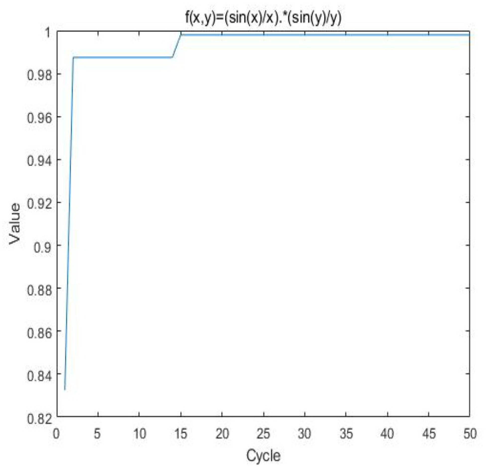
To demonstrate the algorithm’s content, the following numerical example tests the effectiveness of the algorithm. The test function expression is set as

$$f(x,y)=\frac{\sin x}{x}\ast \frac{\sin y}{y},$$

(51)

in which the maximum value point is located at (0,0), and the maximum value is 1.

The initial parameter information is set as follows:

The maximum number of cycles is 50, the importance factor of pheromone $\alpha$ is set as 1, the importance factor of heuristic function $\beta$ is set as 5, pheromone intensity Q is 50, and the volatile factor of pheromone $\rho$ is 0.1.

Figure 1 shows the solution results. As can be seen from Figure 1, after 30 iterations, this is basically close to the maximum extreme value 1, and the solution effectiveness is relatively good.

4.4. A Numerical Example

The following numerical example is given to illustrate the deterministic method proposed in this section.

Example 1.

Consider the following UMP problem

$$\left\{\begin{array}{cc}\underset{x_1,x_2}{min}\hfill & \left(f_1(x,\xi ,\eta ),f_2(x,\vartheta ,\zeta )\right)\hfill \\ \hfill & =(x_2\xi sin(x_1^2-x_2^2)-\sqrt{x_2+\eta x_1}sin(x_2-tan{x}_1),\hfill \\ \hfill & \vartheta cos(\pi x_1-x_2^2+1)+\zeta exp\left\{cos\left(2\pi x_1\right)-\sqrt{x_1^3+2x_2}\right\})\hfill \\ \mathrm{s}.\mathrm{t}.\hfill & x_1^2+x_2^2\le 60,x_1\ge 0,x_2\ge 0,\hfill \end{array}\right.$$

(52)

where $\xi \sim \mathcal{N}(1,\sqrt{3})$, $\eta \sim \mathcal{L}(6,9)$, $\vartheta \sim \mathcal{Z}(6,9,10)$, are linear uncertain variable, normal uncertain variable, and zigzag uncertain variable, respectively, and independent of each other, with uncertainty distributions as follows:

$${\Phi }_{\xi }\left(x\right)={\left(1+exp\left(\frac{\pi \left(1-x\right)}{3}\right)\right)}^{-1},x\in R,$$

(53)

$${\Psi }_{\eta }\left(x\right)\left(x\right)=\left\{\begin{array}{ccc}0,& if\hfill & x\le 6\\ \frac{x-6}{3},& if\hfill & 6\le x\le 9\\ 1,& if\hfill & x\ge 9,\end{array}\right.$$

(54)

and

$${{\rm Y}}_{\vartheta }\left(x\right)=\left\{\begin{array}{ccc}0,& if\hfill & x\le 6\\ \frac{x-6}{6},& if\hfill & 6\le x\le 9\\ \frac{x-8}{2},& if\hfill & 9\le x\le 10\\ 1,& if\hfill & x\ge 10,\end{array}\right.$$

(55)

respectively, and $\zeta =\vartheta exp\left(\eta \right)$.

Discuss the expected-value efficient solution and expected-value variance efficient solution according to the deterministic methods proposed in this section.

First, we used the weighting method to solve Example 1. Since the calculation of the $DS{P}_E^{\left(wm\right)}$ model (33) and that of the $DS{P}_{EV}^{\left(wm\right)}$ model (34) are almost the same, without any losses of generality, we only considered the calculation of the $DS{P}_E^{\left(wm\right)}$ model (33).

According to the $DS{P}_E^{\left(wm\right)}$ model (33), we can obtain

$$\left\{\begin{array}{cc}\underset{x}{min}\hfill & f_E^{\left(wm\right)}\left(x\right)={\omega }_{1}E\left[f_1(x,\xi ,\eta )\right]+{\omega }_{2}E\left[f_2(x,\vartheta ,\zeta )\right]\hfill \\ \hfill & ={\omega }_{1}E\left[x_2\xi sin(x_1^2-x_2^2)-\sqrt{x_2+\eta x_1}sin(x_2-tan{x}_1)\right]\hfill \\ \hfill & +{\omega }_{2}E\left[\vartheta cos(\pi x_1-x_2^2+1)+\zeta exp\left\{cos\left(2\pi x_1\right)-\sqrt{x_1^3+2x_2}\right\}\right]\hfill \\ \mathrm{s}.\mathrm{t}.\hfill & x_1^2+x_2^2\le 60,x_1\ge 0,x_2\ge 0\hfill \\ \hfill & {\omega }_1+{\omega }_2=1,{\omega }_1,{\omega }_2>0.\hfill \end{array}\right.$$

(56)

According to the relevant basic knowledge of uncertainty theory, we calculated the expected value for problems (56).

Since $\xi \sim \mathcal{N}(1,\sqrt{3})$, $\eta \sim \mathcal{L}(6,9)$, $\vartheta \sim \mathcal{Z}(6,9,10)$, are linear uncertain variables, normal uncertain variables, and zigzag uncertain variables, respectively, according to Definition 7, we can obtain the following inverse uncertainty distributions:

$${\Phi }_{\xi }^{-1}\left(\alpha \right)=1+\frac{3}{\pi }ln\frac{\alpha }{1-\alpha },0<\alpha <1,$$

(57)

$${\Psi }_{\eta }^{-1}(1-\alpha )=9-3\alpha ,0<\alpha <1,$$

(58)

and

$${{\rm Y}}_{\vartheta }^{-1}\left(\alpha \right)=\left\{\begin{array}{c}6\alpha +6,0<\alpha <\frac{1}{2}\hfill \\ 2\alpha +8,\frac{1}{2}<\alpha <1,\hfill \end{array}\right.$$

(59)

respectively.

Since $f_1(x,\xi ,\eta )$ is strictly increasing with respect to $\xi$ and strictly decreasing with respect to $\eta$, and $\xi$ and $\eta$ are independent of each other. According the Theorems 4 and 5, we can obtain that

$$\begin{array}{c}E\left[f_1(x,\xi ,\eta )\right]=E\left[x_2\xi sin(x_1^2-x_2^2)-\sqrt{x_2+\eta x_1}sin(x_2-tan{x}_1)\right]\hfill \\ {\displaystyle ={\int }_0^1\left(x_2{\Phi }_{\xi }^{-1}\left(\alpha \right)sin(x_1^2-x_2^2)-\sqrt{x_2+{\Psi }_{\eta }^{-1}(1-\alpha )x_1}sin(x_2-tan{x}_1)\right)d\alpha .}\hfill \end{array}$$

(60)

Since $\zeta =\vartheta exp\left(\eta \right)$, it is easy to know that $\zeta$ and $\vartheta$ are not independent, but the objective function $f_2(x,\xi ,\eta )$ is monotonically increasing with respect to $\zeta$ and $\vartheta$; therefore, according to Theorems 5 and 7, we have

$$\begin{array}{c}E\left[f_2(x,\vartheta ,\zeta )\right]=E\left[\vartheta cos(\pi x_1-x_2^2+1)+\zeta exp\left\{cos\left(2\pi x_1\right)-\sqrt{x_1^3+2x_2}\right\}\right]\hfill \\ {\displaystyle ={\int }_0^1\left({{\rm Y}}_{\vartheta }^{-1}\left(\alpha \right)cos(\pi x_1-x_2^2+1)+{{\rm Y}}_{\vartheta }^{-1}\left(\alpha \right)exp\left\{{\Phi }_{\eta }^{-1}\left(\alpha \right)\right\}exp\left\{cos\left(2\pi x_1\right)-\sqrt{x_1^3+2x_2}\right\}\right)d\alpha .}\hfill \end{array}$$

(61)

From the above analysis, the problems (56) are equivalent to the following problem:

$$\left\{\begin{array}{cc}\underset{x}{min}\hfill & f_E^{\left(wm\right)}\left(x\right)={\omega }_{1}E\left[f_1(x,\xi ,\eta )\right]+{\omega }_{2}E\left[f_2(x,\vartheta ,\zeta )\right]\hfill \\ \hfill & {\displaystyle ={\omega }_1{\int }_0^1\left(x_2{\Phi }_{\xi }^{-1}\left(\alpha \right)sin\left(x_1^2-x_2^2\right)-\sqrt{x_2+{\Psi }_{\eta }^{-1}(1-\alpha )x_1}sin(x_2-tan{x}_1)\right)d\alpha }\hfill \\ \hfill & {\displaystyle +{\omega }_2{\int }_0^1({{\rm Y}}_{\vartheta }^{-1}\left(\alpha \right)cos(\pi x_1-x_2^2+1)}\hfill \\ \hfill & +{{\rm Y}}_{\vartheta }^{-1}\left(\alpha \right)exp\left\{{\Phi }_{\eta }^{-1}\left(\alpha \right)\right\}exp\left\{cos\left(2\pi x_1\right)-\sqrt{x_1^3+2x_2}\right\})d\alpha \hfill \\ \mathrm{s}.\mathrm{t}.\hfill & x_1^2+x_2^2\le 60,x_1\ge 0,x_2\ge 0\hfill \\ \hfill & {\omega }_1+{\omega }_2=1,{\omega }_1,{\omega }_2>0.\hfill \end{array}\right.$$

(62)

By using the AC algorithm and considering the five sets of weights, we obtain the corresponding optimal solutions to the problem (62), as shown in

Table 1. The results using the weighting method in deterministic method.

Wights	Optimal Solutions	Objective Values
$({\omega }_1,{\omega }_2)=(0.95,0.05)$	$x^{*}={(4.7821,6.0893)}^T$	−12.1434
$({\omega }_1,{\omega }_2)=(0.80,0.20)$	$x^{*}={(4.7821,6.0936)}^T$	−10.9964
$({\omega }_1,{\omega }_2)=(0.60,0.40)$	$x^{*}={(4.8296,5.6162)}^T$	−10.0055
$({\omega }_1,{\omega }_2)=(0.40,0.60)$	$x^{*}={(7.0739,2.7447)}^T$	−9.1356
$({\omega }_1,{\omega }_2)=(0.25,0.75)$	$x^{*}={(7.0731,2.7426)}^T$	−8.8969
$({\omega }_1,{\omega }_2)=(0.10,0.90)$	$x^{*}={(7.0726,2.7412)}^T$	−8.6585

. According to Definition 9 and Theorem 12, these five sets of optimal solutions are also expected-value efficient solutions to initial UMP problem (52).

As can be seen from the results in Table 1, if we think that the first objective function is more important, the optimal decisions we take are $x^{*}={(4.7821,6.0893)}^T$ and $x^{*}={(4.7821,6.0936)}^T$; if we think that the second objective function is more important, the optimal decisions are $x^{*}={(7.0731,2.7426)}^T$ and $x^{*}={(7.0726,2.7412)}^T$; otherwise, decisions $x^{*}={(4.8296,5.6162)}^T$ and $x^{*}={(7.0739,2.7447)}^T$ are reasonable.

Next, the ideal-point method in the deterministic method was used to solve Example 1. Since the calculation of $DS{P}_E^{\left(ipm\right)}$ model (41) and that of the $DS{P}_{EV}^{\left(ipm\right)}$ model (42) are almost the same, without any losses of generality, we only considered the calculation of the $DS{P}_E^{\left(ipm\right)}$ model (41).

Under the ideal point preference, the ideal values of objective functions in the $DS{P}_E^{\left(ipm\right)}$ model (41) should be obtained by solving the following two single-objective programmings:

$$\left\{\begin{array}{cc}\underset{x}{min}\hfill & E\left[f_1(x,\xi ,\eta )\right]\hfill \\ \hfill & {\displaystyle ={\int }_0^1\left(x_2{\Phi }_{\xi }^{-1}\left(\alpha \right)sin\left(x_1^2-x_2^2\right)-\sqrt{x_2+{\Psi }_{\eta }^{-1}(1-\alpha )x_1}sin\left(x_2-tan{x}_1\right)\right)d\alpha }\hfill \\ \mathrm{s}.\mathrm{t}.\hfill & x_1^2+x_2^2\le 60,x_1\ge 0,x_2\ge 0\hfill \end{array}\right.$$

(63)

and

$$\left\{\begin{array}{c}\underset{x}{min}E\left[f_2(x,\vartheta ,\zeta )\right]\hfill \\ {\displaystyle =={\int }_0^1\left({{\rm Y}}_{\vartheta }^{-1}\left(\alpha \right)cos(\pi x_1-x_2^2+1)+{{\rm Y}}_{\vartheta }^{-1}\left(\alpha \right)exp\left\{{\Psi }_{\eta }^{-1}\left(\alpha \right)\right\}exp\left\{cos\left(2\pi x_1\right)-\sqrt{x_1^3+2x_2}\right\}\right)d\alpha }\hfill \\ \mathrm{s}.\mathrm{t}.x_1^2+x_2^2\le 60,x_1\ge 0,x_2\ge 0.\hfill \end{array}\right.$$

(64)

By suing the AC algorithm designed in Section 4.3, we obtain

$$\underset{x}{min}E\left[f_1(x,\xi ,\eta )\right]=-12.5526,\underset{x}{min}E\left[f_2(x,\vartheta ,\zeta )\right]=-8.4998.$$

(65)

According to the practical meaning of the ideal point values, we take $f_1^{\left(e_0\right)}$ as −12.5526 and $f_2^{\left(e_0\right)}$ as −8.4998. Hence, we can obtain the $DS{P}_E^{\left(ipm\right)}$ model (41) as follows:

$$\left\{\begin{array}{cc}\underset{x}{min}\hfill & {\mathit{f}}_E^{\left(ipm\right)}\left(x\right)={\left({\left(E\left[f_1(x,\xi ,\eta )\right]-f_1^{\left(e_0\right)}\right)}^2+{\left(E\left[f_2(x,\vartheta ,\zeta )\right]-f_2^{\left(e_0\right)}\right)}^2\right)}^{\frac{1}{2}}\hfill \\ \hfill & {\displaystyle =\left(\right({\int }_0^1(x_2{\Phi }_{\xi }^{-1}\left(\alpha \right)sin(x_1^2-x_2^2)}\hfill \\ \hfill & -\sqrt{x_2+{\Psi }_{\eta }^{-1}(1-\alpha )x_1}sin(x_2-tan{x}_1))d\alpha +12.5526{)}^2\hfill \\ \hfill & {\displaystyle +\left({\int }_0^1\right({{\rm Y}}_{\vartheta }^{-1}\left(\alpha \right)cos(\pi x_1-x_2^2+1)}\hfill \\ \hfill & +{\Psi }_{\vartheta }^{-1}\left(\alpha \right)exp\left\{{\Phi }_{\eta }^{-1}\left(\alpha \right)\right\}exp\left\{cos\left(2\pi x_1\right)-\sqrt{x_1^3+2x_2}\right\})d\alpha +8.4998{)}^2{)}^{\frac{1}{2}}\hfill \\ \mathrm{s}.\mathrm{t}.\hfill & x_1^2+x_2^2\le 60,x_1\ge 0,x_2\ge 0.\hfill \end{array}\right.$$

(66)

By using the AC algorithm, we obtain that the optimal solution $x^{*}$ to the problem (66) is ${(5.0453,5.1594)}^T$, and the corresponding objective function value is 1.7002. According to Definition 9 and Theorem 13, this optimal solution is also the expected-value efficient solution of the initial UMP problem (52) under ideal point preference.

It can be seen from the comparison that the expected-value efficient solutions under weighting preference in Table 1 were obviously different from the expected-value efficient solutions under ideal-point preference. These two types of efficient solutions are not good or bad, but only represent the different preferences taken by the decision-maker. The choice between methods should be made according to the practical problems in the real world.

5. Uncertain Method for Solving Uncertain Multiobjective Programming

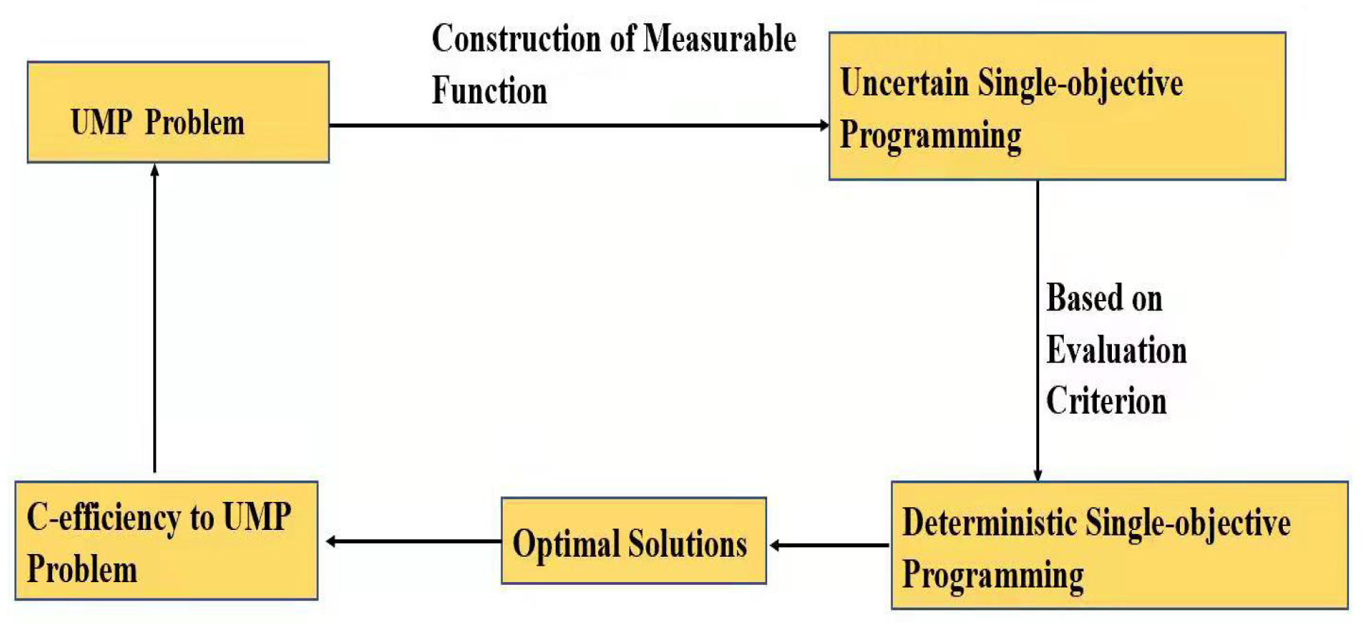
It can be seen from Section 4 that the general idea of the deterministic method is as follows:

The initial UMP problem (18) is first transformed into a deterministic multiobjective programming problem (21) (or problem (24)) by the expectation (or variance) of the uncertain objective function, and then the problem (21) (or problem (24)) is converted into a deterministic single-objective, programming the problem (33) (or problem (41)) according to the weighting method (or ideal point method). Finally, the expected-value efficient solutions (or expected-value variance efficient solutions) are obtained by solving the problem (33) (or problem (41)). Figure 2 shows the idea of the deterministic method.

However, as shown in Figure 2, the uncertain objective functions in the UMP problem (18) are transformed into mutually independent deterministic objective functions. When the uncertainties between uncertain objective functions are closely related, the deterministic method cuts off the uncertainty relation between them. Therefore, the final decisions are obviously not in line with reality. 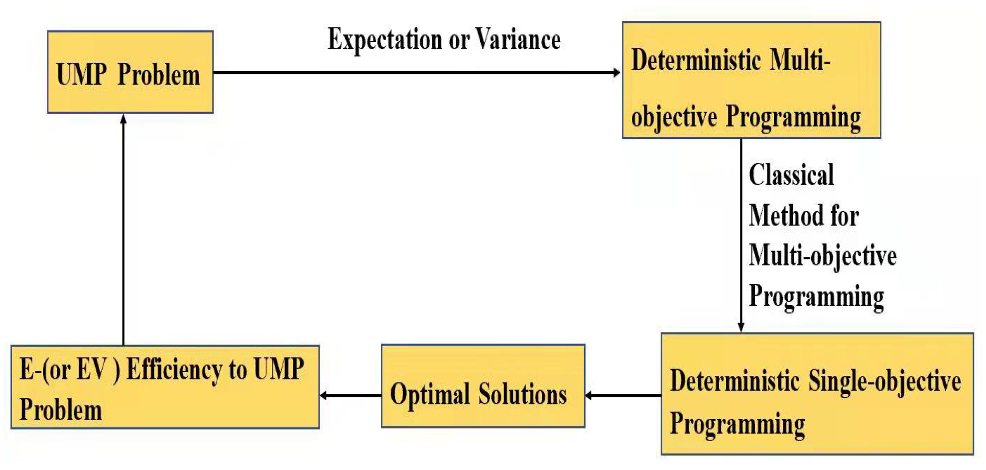To overcome this disadvantage of the deterministic method, the uncertain method is proposed in this section. The main idea of this method is as follows:

Firstly, by constructing a measure function $G(·)$, we transform the UMP problem (18) into an uncertain single-objective programming (USP) problem, that is,

$$\left\{\begin{array}{cc}\underset{x}{min}\hfill & G\left(f_1(x,{\mathbf{\xi }}_1),f_2(x,{\mathbf{\xi }}_2),\cdots ,f_s(x,{\mathbf{\xi }}_s)\right)\hfill \\ \mathrm{s}.\mathrm{t}.\hfill & x\in S.\hfill \end{array}\right.$$

(67)

Secondly, the USP problem (67) is transformed into a deterministic single-objective programming (DSP) problem using the proposed evaluation criterion C, and optimal solutions are obtained by solving the DSP problem. Further, we prove that the optimal solutions to the DSP problem are C-efficient solutions to the initial UMP problem (18). Figure 3 shows the idea of the uncertain method.

From the comparison between Figure 2 and Figure 3, it can be seen that the deterministic method ignores the uncertain connection between the objective functions in the initial UMP problem from the first step, while the uncertain method considers that from the beginning to the end.

5.1. Order Relationship between Uncertain Variables

The first step of the uncertain method is to transform the initial UMP problem (18) into the USP problem (67) through a measurable function G. Since uncertain variables cannot be directly compared, to solve the USP problem (67), the comparison method between the uncertain variables according to the evaluation value of objective functions in the real decision-making process should be given first. This is the order relationship between uncertain variables.

In this paper, “≺” and “⪯” are used to represent the order relationship between two uncertain variables. For example, under a given evaluation criterion, if $f(x_1,\mathbf{\xi })\prec f(x_2,\mathbf{\xi })$, we say that the evaluation value (or loss value, etc.) of the uncertain variable $f(x_1,\mathbf{\xi })$ is strictly superior to that of the uncertain variable $f(x_2,\mathbf{\xi })$, and if $f(x_1,\mathbf{\xi })⪯f(x_2,\mathbf{\xi })$, we say that the evaluation value (or loss value, etc.) of the uncertain variable $f(x_1,\mathbf{\xi })$ is not worse than that of uncertain variable $f(x_2,\mathbf{\xi })$.

Definition 13.

Assume that ξ and η are uncertain variables. We define that

$$\xi \prec (⪯)\eta$$

(68)

if, and only if,

$$C\left(\xi \right)<(\leqq )C\left(\eta \right),$$

(69)

where C is an evaluation criterion used to compare uncertain variables, and $C(·)$ represents the evaluation value.

Remark 1.

According to Definition 13, $\xi \prec \eta$ means that the evaluation value $C\left(\xi \right)$ is strictly less than $C\left(\eta \right)$, while $\xi ⪯\eta$ means that the evaluation value $C\left(\xi \right)$ is no greater than $C\left(\eta \right)$. Further, evaluation criterion C is a general term, which determines the order relationship between uncertain variables. The evaluation criteria given by different practical problems also differ according to different practical needs. For example, considering the product design problem under the uncertain environment, it is necessary to create an optimal design scheme to minimize the cost $P(x,\mathbf{\xi })$ over a long period of time. In this case, the expected-value criterion (denoted as $C_E$) should be used to provide the order relationship between uncertain variables. If

$$P(x_1,\mathbf{\xi })\prec P(x_2,\mathbf{\xi }),$$

(70)

then we can see that the average cost caused by decision-making $x_1$ is strictly lower than that cased by decision-making $x_2$; that is, under the $C_E$ criterion, uncertain variable $P(x_1,\mathbf{\xi })$ is strictly superior to the uncertain variable $P(x_2,\mathbf{\xi })$. Similarly, if we are concerned with the fluctuations in the cost of the objective function $P(x,\mathbf{\xi })$, then the variance criterion $C_V$ should be used to provide the order relationship between uncertain variables. If

$$P(x_1,\mathbf{\xi })\prec P(x_2,\mathbf{\xi }),$$

(71)

then we can see that the fluctuations in the cost caused by decision-making $x_1$ are strictly lower than that cased by decision-making $x_2$, that is, under the $C_V$ criterion, uncertain variable $P(x_1,\mathbf{\xi })$ is strictly superior to uncertain variable $P(x_2,\mathbf{\xi })$.

The following definitions are the order relationship between uncertain variables according to the common evaluation criteria in the practical problem.

Definition 14 (${\mathit{C}}_{\mathit{E}}$ Criterion).

Assuming that ξ and η are two uncertain variables, we define that

$$\xi \prec (⪯)\eta$$

(72)

if and only if

$$E\left[\xi \right]<(\leqq )E\left[\eta \right],$$

(73)

where $E[·]$ denotes the expected value of the uncertain variable.

Definition 15 (${\mathit{C}}_{\mathit{V}}$ Criterion).

Assuming that ξ and η are two uncertain variables, we define that

$$\xi \prec (⪯)\eta$$

(74)

if and only if

$$V\left[\xi \right]<(\leqq )V\left[\eta \right],$$

(75)

where $V[·]$ denotes the variance of the uncertain variable.

Definition 16 (${\mathit{C}}_{{\mathbf{\alpha }}_{sup}}$ Criterion).

Assuming that ξ and η are two uncertain variables, we define that

$$\xi \prec (or⪯)\eta$$

(76)

if and only if

$${\xi }_{sup}\left(\alpha \right)<(or\le ){\eta }_{sup}\left(\alpha \right)$$

(77)

for a given confidence level $\alpha \in (0,1]$, where ${\xi }_{sup}\left(\alpha \right)$ and ${\eta }_{sup}\left(\alpha \right)$ denote the α-optimistic value of uncertain variables ξ and η, respectively.

Definition 17 (${\mathit{C}}_{{\mathbf{\alpha }}_{inf}}$ Criterion).

Assuming that ξ and η are two uncertain variables, we define that

$$\xi \prec (or⪯)\eta$$

(78)

if and only if

$${\xi }_{inf}\left(\alpha \right)<(or\le ){\eta }_{inf}\left(\alpha \right)$$

(79)

for a given confidence level $\alpha \in (0,1]$, where ${\xi }_{inf}\left(\alpha \right)$ and ${\eta }_{inf}\left(\alpha \right)$ denote the α-pessimistic value of uncertain variables ξ and η, respectively.

Based on the order relationship between uncertain variables, the optimal solution to the USP problem (67) and efficient solution to the UMP problem (18) can be defined.

Definition 18.

Based on the given C criterion, a feasible solution $x^{*}$ is called the C-optimal (or strictly C-optimal) solution to the USP problem (67) if

$$G\left(f_1(x^{*},{\mathbf{\xi }}_1),f_2(x^{*},{\mathbf{\xi }}_2),\cdots ,f_s(x^{*},{\mathbf{\xi }}_s)\right)\prec (or⪯)G\left(f_1(x,{\mathbf{\xi }}_1),f_2(x,{\mathbf{\xi }}_2),\cdots ,f_s(x,{\mathbf{\xi }}_s)\right)$$

(80)

for any feasible solution $x\in S$.

Definition 19.

Based on the given C criterion, a feasible solution $x^{*}$ is called the C-efficient solution to the UMP problem (18) if there is no feasible solution $x\in S$ such that

$$f_i(x^{*},{\mathbf{\xi }}_i)⪯f_i(x,{\mathbf{\xi }}_i),1\le i\le s,$$

(81)

and

$$f_{i_0}(\overline{x},{\mathbf{\xi }}_{i_0})\prec f_{i_0}(x^{*},{\mathbf{\xi }}_{i_0}).$$

(82)

for at least one $i_0,1\le i_0\le s$.

Since the average-based evaluation criterion is very common in practical problems, this paper mainly considers the expected-value criterion $C_E$. Therefore, all C evaluation criteria in the latter part of this paper represent the expected-value criterion $C_E$ without it being explicitly stated; that is, “$\prec or⪯$” represents the order relationship between uncertain variables based on the $C_E$ criterion.

The second step in the uncertain method is constructing the measurable function G. Next, two types of commonly used construction methods, that is, the linear weighted construction method (LWCM) and ideal point construction method (IPCM), will be given.

5.2. Linear Weighted Construction Method

We constructed the measure function G by providing each objective function with their corresponding weight, and the following uncertain single-objective programming ($US{P}^{\left(lwcm\right)}$) could be obtained:

$$\left(US{P}^{\left(lwcm\right)}\right)\left\{\begin{array}{cc}\underset{x}{min}\hfill & G^{\left(lwcm\right)}\left(f_1(x,{\mathbf{\xi }}_1),f_2(x,{\mathbf{\xi }}_2),\cdots ,f_s(x,{\mathbf{\xi }}_s)\right)\hfill \\ \hfill & ={\displaystyle \sum _{i=1}^s}{\alpha }_i{f}_i(x,{\mathbf{\xi }}_i)\hfill \\ \mathrm{s}.\mathrm{t}.\hfill & {\displaystyle \sum _{i=1}^s}{\alpha }_k=1,{\alpha }_i>0,i=1,2,\cdots ,s\hfill \\ \hfill & x\in S.\hfill \end{array}\right.$$

(83)

Based on the $C_E$ criterion, the $US{P}^{\left(lwcm\right)}$ problem (83) is equivalent to the following deterministic single-objective programming

$$\left(US{P}^{\left(lwcm\right)}\right)\left\{\begin{array}{cc}\underset{x}{min}\hfill & E\left[G^{\left(lwcm\right)}\left(f_1(x,{\mathbf{\xi }}_1),f_2(x,{\mathbf{\xi }}_2),\cdots ,f_s(x,{\mathbf{\xi }}_s)\right)\right]\hfill \\ \hfill & =E\left[{\displaystyle \sum _{i=1}^s}{\alpha }_i{f}_i(x,{\mathbf{\xi }}_i)\right]\hfill \\ \mathrm{s}.\mathrm{t}.\hfill & {\displaystyle \sum _{i=1}^s}{\alpha }_k=1,{\alpha }_i>0,i=1,2,\cdots ,s\hfill \\ \hfill & x\in S.\hfill \end{array}\right.$$

(84)

Based on the $C_E$ evaluation criterion, to provide the relations between the $C_E$-optimal solution of the USP problem (84) and $C_E$-efficient solution of UMP problem (18), the following lemmas are first proposed first:

Lemma 1.

Assume that f is a measurable function, and ξ is an uncertain variable. If $f(x^{*},\xi )\prec (or⪯)f(x,\xi )$, then we have

$$\alpha f(x^{*},\xi )\prec (or⪯)\alpha f(x,\xi )$$

(85)

for any real number ${\alpha }_i>0$ and any feasible decision-making $x^{*}$, $x\in S$.

Proof. 

Since $f(x^{*},\xi )\prec (or⪯)f(x,\xi )$, according to the definition of the $C_E$ criterion, we have

$$E\left[f(x^{*},\xi )\right]<(or\le )E\left[f(x,\xi )\right].$$

(86)

For any real number ${\alpha }_i>0$, by Theorem 2.6, we have

$$E\left[\alpha f(x^{*},\xi )\right]<(\le )E\left[\alpha f(x,\xi )\right],$$

(87)

which implies that

$$\alpha f(x^{*},\xi )\prec (or⪯)\alpha f(x,\xi ).$$

(88)

This lemma is complete.  □

Lemma 2.

Assume that f is a measurable function, $f(x_1,\xi )$ and $f(x_2,\xi )$ are uncertain variables with regular uncertainty distributions ${\Phi }_1$ and ${\Phi }_2$, $f(x_1,\eta )$ and $f(x_2,\eta )$ are uncertain variables with regular uncertainty distributions ${\Psi }_1$ and ${\Psi }_2$. Further, suppose that $f(x,\xi )$ strictly increases with respect to ξ, and $f(x,\eta )$ is a strictly decreasing function with respect to η. If

$$f(x_1,\xi )\prec (or⪯)f(x_2,\xi ),f(x_1,\eta )\prec (or⪯)f(x_2,\eta ),$$

(89)

then we have

$$f(x_1,\xi )+f(x_1,\eta )\prec (or⪯)f(x_2,\xi )+f(x_2,\eta ).$$

(90)

Proof. 

Since

$$f(x_1,\xi )\prec (or⪯)f(x_2,\xi ),f(x_1,\eta )\prec (or⪯)f(x_2,\eta ),$$

(91)

according to the $C_E$ criterion, we have

$$E\left[f(x_1,\xi )\right]<(or\le )E\left[f(x_2,\xi )\right],E\left[f(x_1,\eta )\right]<(or\le )E\left[f(x_2,\eta )\right].$$

(92)

It follows from Theorems 4 and 5 that

$${\int }_0^1{\Phi }_1^{-1}\left(\alpha \right)d\alpha <(or\le ){\int }_0^1{\Phi }_2^{-1}\left(\alpha \right)d\alpha ,$$

(93)

and

$${\int }_0^1{\Psi }_1^{-1}(1-\alpha )d\alpha <(or\le ){\int }_0^1{\Psi }_2^{-1}(1-\alpha )d\alpha .$$

(94)

Evidently,

$$\begin{array}{cc}& {\int }_0^1\left({\Phi }_1^{-1}\left(\alpha \right)+{\Psi }_1^{-1}(1-\alpha )\right)d\alpha \hfill \\ \hfill <(or\le )& {\int }_0^1\left({\Phi }_2^{-1}\left(\alpha \right)+{\Psi }_2^{-1}(1-\alpha )\right)d\alpha .\hfill \end{array}$$

(95)

Using Theorem 6, we can obtain

$$E[f(x_1,\xi )+f(x_1,\eta )]<(or\le )E[f(x_2,\xi )+f(x_2,\eta )],$$

(96)

which implies, according the definition of $C_E$ criterion, that

$$f(x_1,\xi )+f(x_1,\eta )\prec (or⪯)f(x_2,\xi )+f(x_2,\eta ).$$

(97)

The lemma is proved.  □

Theorem 14.

The $C_E$-optimal solution $x^{*}$ to the $US{P}^{\left(lwcm\right)}$ problem (84) must be the $C_E$-efficient solution to the initial UMP problem (18).

Proof. 

Assume that $x^{*}$ is $C_E$-optimal solution to the $US{P}^{\left(lwcm\right)}$ problem (84) but not the $C_E$-efficient solution to the initial problem (18). According to Definition 19, there must be a feasible solution $\overline{x}\in S$, such that

$$f_i(\overline{x},{\xi }_i)⪯f_i(x^{*},{\xi }_i),1\le i\le s,$$

(98)

and

$$f_{i_0}(\overline{x},{\xi }_{i_0})\prec f_{i_0}(x^{*},{\xi }_{i_0}).$$

(99)

for at least one $i_0,1\le i_0\le s$.

Since ${\alpha }_i>0$, $k=1,2,\cdots ,s$, according to Lemmas 1 and 2, we can obtain that

$$\sum _{i=1}^s{\alpha }_i{f}_i(\overline{x},{\xi }_i)\prec {\alpha }_1\sum _{i=1}^s{\alpha }_i{f}_i(x^{*},{\xi }_i).$$

(100)

Hence,

$$\begin{array}{c}\hfill G^{\left(lwcm\right)}\left(f_1(\overline{x},{\xi }_1),f_2(\overline{x},{\xi }_2),\cdots ,f_s(\overline{x},{\xi }_s)\right)\\ \hfill \prec G^{\left(lwcm\right)}\left(f_1(x^{*},{\xi }_1),f_2(x^{*},{\xi }_2),\cdots ,f_s(x^{*},{\xi }_s)\right)\end{array}$$

(101)

which contradicts the idea that $x^{*}$ is $C_E$-optimal solution to the $US{P}^{\left(lwcm\right)}$ problem (84); hence, the $C_E$-optimal solution $x^{*}$ to the $US{P}^{\left(lwcm\right)}$ problem (84) is the $C_E$-efficient solution to the initial problem (18). The theorem is proved.  □

From the analysis, we can see that the $US{P}^{\left(lwcm\right)}$ problem (83) first takes the weighted sum, and then its expectation, while the $DS{P}_E^{\left(wm\right)}$ problem (33) is the opposite. According to the properties of the expectation of an uncertain variable, which can be referred to using Theorems 5 and 6, except for the cases where uncertain variable $f_i(x,{\xi }_i),1\le i\le s$ is independent or comonotonic with respect to ${\xi }_i$, we have

$$E\left[\sum _{i=1}^s{\alpha }_i{f}_i(x,{\xi }_i)\right]\ne \sum _{i=1}^s{\alpha }_{i}E\left[f_i(x,{\xi }_i)\right],$$

(102)

which differs from the expectation properties in stochastic systems. Therefore, even if we adopt the $C_E$ criterion, the $US{P}^{\left(lwcm\right)}$ problem (83) is completely different from the $DS{P}_E^{\left(wm\right)}$ problem (33).

From the above analysis, it can be seen that the results obtained in this paper are different from those in the literature [24]. In the literature [24], based on the expected value criterion of random variables, the efficient solutions to the stochastic multiobjective programming obtained by these two types of solution methods are exactly the same under the preference of the weight method. As stated in the introduction, unlike random variables, the expected value of uncertain variables does not have linear properties; even with the expected value criterion and the weight method used, the efficient solutions obtained by the two types of solution method are different.

5.3. Ideal Point Construction Method

In the practical decision-making problem, it is assumed that the objective functions in the ideal point method are an important preference method, differing from the weighted method, which is also very important in practical decision-making problems. It is easy to see that, using the ideal point construction method, the efficient solutions obtained by these two types of solution method are obviously different. This has not been studied in the previous research work, such as reference [23,24].

Assuming that objective functions in the E-UMP problem (21) or EV-UMP problem (24) have their ideal values, then the best decision-making scheme is to make all the objective functions meet the corresponding ideal values. However, since the objective functions in the E-UMP problem (21) or EV-UMP problem (24) are usually conflicting and contradictory, this best decision-making scheme often does not exist. Hence, the next best thing is to find a sub-optimal decision-making scheme that makes the objective functions match their ideal objective values as closely as possible.

Assuming that the uncertain objective function $f_i(x,{\mathbf{\xi }}_i)$ has the ideal value $f_i^{\left(0\right)}$, the best decision-making satisfies the $f_i^{\left(0\right)}=f_i(x,{\mathbf{\xi }}_i),$ as far as possible; that is, we need to solve the following uncertain single-objective programming ($US{P}^{ipcm}$) problem:

$$\left(US{P}^{\left(ipcm\right)}\right)\left\{\begin{array}{cc}\underset{x}{min}\hfill & G^{\left(ipcm\right)}\left(f_1(x,{\mathbf{\xi }}_1),f_2(x,{\mathbf{\xi }}_2),\cdots ,f_s(x,{\mathbf{\xi }}_s)\right)\hfill \\ \hfill & ={\left({\displaystyle \sum _{i=1}^s}{\left(f_i(x,\mathbf{\xi })-f_i^{\left(0\right)}\right)}^2\right)}^{\frac{1}{2}}\hfill \\ \mathrm{s}.\mathrm{t}.\hfill & x\in S.\hfill \end{array}\right.$$

(103)

where

$$f_i^{\left(0\right)}\le \underset{x}{min}{f}_i(x,\mathbf{\xi }),1\le i\le s.$$

Based on the $C_E$ criterion, the $US{P}^{\left(ipcm\right)}$ problem (103) is equivalent to the following deterministic single-objective programming problem:

$$\left(US{P}^{\left(ipcm\right)}\right)\left\{\begin{array}{cc}\underset{x}{min}\hfill & E\left[G^{\left(ipcm\right)}\left(f_1(x,{\mathbf{\xi }}_1),f_2(x,{\mathbf{\xi }}_2),\cdots ,f_s(x,{\mathbf{\xi }}_s)\right)\right]\hfill \\ \hfill & =E\left[{\left({\displaystyle \sum _{i=1}^s}{\left(f_i(x,\mathbf{\xi })-f_i^{\left(0\right)}\right)}^2\right)}^{\frac{1}{2}}\right]\hfill \\ \mathrm{s}.\mathrm{t}.\hfill & x\in S.\hfill \end{array}\right.$$

(104)

Based on the $C_E$ criterion, to provide the relations between the $C_E$-optimal solution of $US{P}^{ipcm}$ problem (104) and the $C_E$-efficient solution of UMP problem (18). The following lemmas are proved first.

Lemma 3.

Assuming that f is a measurable function, $f(x,\xi )$ and $f(x,\eta )$ are uncertain variables with regular uncertainty distributions $\Phi$ and $\Psi$, respectively. Further, suppose that $f(x,\xi )$ is strictly increasing with respect to ξ, and $f(x,\eta )$ is a strictly decreasing function with respect to η. If $f(x,\xi )\prec (or⪯)f(x,\eta )$, and the lower bounds of $f(x,\xi )$ and $f(x,\eta )$ exist. Then, for any real number $f^0\le min\{inff(x,\xi ),inff(x,\eta )\}$, we have

$${\left(f(x,\xi )-f^0\right)}^2\prec (or⪯){\left(f(x,\eta )-f^0\right)}^2.$$

(105)

Proof. 

Since $f(x,\xi )\prec (or⪯)f(x,\eta )$, by the definition of $C_E$ criterion, we have

$$E\left[f\right(x,\xi \left)\right]<(or\leqq )E\left[f\right(x,\eta \left)\right].$$

(106)

It follows from Theorems 3 and 4 that

$${\int }_0^1{\Phi }^{-1}\left(\alpha \right)d\alpha <{\int }_0^1{\Psi }^{-1}(1-\alpha )d\alpha .$$

(107)

Since $f^0\le min\{inff(x,\xi ),inff(x,\eta )\}$, according to the definition of inverse uncertainty distribution, we know that $f^0\le min\{inf{\Phi }^{-1}\left(\alpha \right),inf{\Psi }^{-1}(1-\alpha )\}$. Hence,

$${\int }_0^1{\left({\Phi }^{-1}\left(\alpha \right)-f^0\right)}^{2}d\alpha <(or\le ){\int }_0^1{\left({\Psi }^{-1}(1-\alpha )-f^0\right)}^{2}d\alpha$$

(108)

Hence, according to Theorem 4, we have

$${\int }_0^1{({\Phi }^{-1}\left(\alpha \right)-f^0)}^{2}d\alpha =E\left[{(f(x,\xi )-f^0)}^2\right]$$

(109)

and

$${\int }_0^1{({\Psi }^{-1}\left(\alpha \right)-f^0)}^{2}d\alpha =E\left[{(f(x,\eta )-f^0)}^2\right].$$

(110)

It is easily obtained that

$$E\left[{(f(x,\xi )-f^0)}^2\right]<(or\le )E\left[{(f(x,\xi )-f^0)}^2\right]$$

(111)

that is,

$${\left(f(x,\xi )-f^0\right)}^2\prec (or⪯){\left(f(x,\eta )-f^0\right)}^2.$$

(112)

The theorem is complete.  □

Lemma 4.

Assuming that f is a measurable function, $f(x,\xi )$ and $f(x,\eta )$ both are nonnegative uncertain variables with regular uncertainty distributions $\Phi$ and $\Psi$. Further, suppose that $f(x,\xi )$ is strictly increasing with respect to ξ, and $f(x,\eta )$ is strictly decreasing with respect to η. If $f(x,\xi )\prec (or⪯)f(x,\eta )$, then we have

$$\sqrt{f(x,\xi )}\prec (or⪯)\sqrt{f(x,\eta )}.$$

(113)

Proof. 

Since $f(x,\xi )\prec (or⪯)f(x,\eta )$, according to the definition of $C_E$ criterion, we have

$$E\left[f\right(x,\xi \left)\right]\le (or<)E\left[f\right(x,\eta \left)\right].$$

(114)

It follows from Theorems 3 and 4 that

$${\int }_0^1{\Phi }^{-1}\left(\alpha \right)d\alpha <(or\le ){\int }_0^1{\Psi }^{-1}(1-\alpha )d\alpha .$$

(115)

Since $f(x,\xi )$ and $f(x,\eta )$ are both nonnegative, and $\sqrt{{\Phi }^{-1}\left(\alpha \right)}$ and $\sqrt{{\Psi }^{-1}(1-\alpha )}$ exist, we have

$${\int }_0^1\sqrt{{\Phi }^{-1}\left(\alpha \right)}d\alpha <(or\le ){\int }_0^1\sqrt{{\Psi }^{-1}(1-\alpha )}d\alpha .$$

(116)

Since $\sqrt{x}$ is a strictly increasing function, $f(x,\xi )$ is strictly increasing with respect to $\xi$, and $f(x,\eta )$ is strictly decreasing with respect to $\eta$, it follows from Theorems 3 and 5 that

$${\int }_0^1\sqrt{{\Phi }^{-1}\left(\alpha \right)}d\alpha =E\left[\sqrt{f(x,\xi )}\right],{\int }_0^1\sqrt{{\Psi }^{-1}(1-\alpha )}d\alpha =E\left[\sqrt{f(x,\eta )}\right].$$

(117)

Evidently,

$$E\left[\sqrt{f(x,\xi )}\right]<(or\le )E\left[\sqrt{f(x,\eta )}\right],$$

(118)

which implies, according t the definition of $C_E$ criterion, that

$$\sqrt{f(x,\xi )}\prec (or⪯)\sqrt{f(x,\eta )}.$$

(119)

The lemma is proved.  □

Theorem 15.

The $C_E$-optimal solution $x^{*}$ to the $US{P}^{\left(ipcm\right)}$ problem (104) must be the $C_E$-efficient solution to the initial UMP problem (18).

Proof. 

Assume that $x^{*}$ is $C_E$-optimal solution to the $US{P}^{\left(ipcm\right)}$ problem (84) but not the $C_E$-efficient solution to the initial problem (1). According to Definition 19, there must be a feasible solution $\overline{x}\in S$ such that

$$f_i(\overline{x},{\xi }_i)⪯f_i(x^{*},{\xi }_i),1\le i\le s,$$

(120)

and

$$f_{i_0}(\overline{x},{\xi }_{i_0})\prec f_{i_0}(x^{*},{\xi }_{i_0}).$$

(121)

for at least one $i_0,1\le i_0\le s$.

Since

$$f_i^{\left(0\right)}\le \underset{i}{inf}{f}_i(x,\mathbf{\xi }),1\le i\le s,$$

(122)

we can obtain, according to Lemmas 3 and 4, that

$$\sqrt{\sum _{i=1}^s(f_i(\overline{x},\xi )-f_i^{\left(0\right)}{)}^2}\prec \sqrt{\sum _{i=1}^s(f_i(x^{*},\xi )-f_i^{\left(0\right)}{)}^2}.$$

(123)

According to $US{P}^{\left(ipcm\right)}$ (104), we have

$$\begin{array}{c}\hfill G^{\left(ipcm\right)}\left(f_1(\overline{x},{\xi }_1),f_2(\overline{x},{\xi }_2),\cdots ,f_s(\overline{x},{\xi }_s)\right)\\ \hfill \prec G^{\left(ipcm\right)}\left(f_1(x^{*},{\xi }_1),f_2(x^{*},{\xi }_2),\cdots ,f_s(x^{*},{\xi }_s)\right)\end{array}$$

(124)

which contradicts the idea that $x^{*}$ is a $C_E$-optimal solution to the $US{P}^{\left(ipcm\right)}$ problem (104); hence, the $C_E$-optimal solution $x^{*}$ to the $US{P}^{\left(ipcm\right)}$ problem (104) is the $C_E$-efficient solution to the initial problem (18). The theorem is proved.  □

It is easy to see from problem (104) and problem (41) that the ideal point construction method of the uncertain method obviously differs from the ideal-point method of the deterministic method. Problem (104) first minimizes the sum of squares of errors and then uses its expectation, while problem (41) does the opposite. Generally speaking, we have

$$E\left[{\left(\sum _{i=1}^s{\left(f_i(x,\mathbf{\xi })-f_i^{\left(0\right)}\right)}^2\right)}^{\frac{1}{2}}\right]\ne {\left(\sum _{i=1}^s{\left(E\left[f_i(x,\mathbf{\xi })\right]-f_i^{\left(0\right)}\right)}^2\right)}^{\frac{1}{2}}.$$

(125)

Hence, even if we adopt the $C_E$ criterion, the $US{P}^{\left(ipcm\right)}$ problem (103) is completely different from the $DS{P}_E^{\left(ipm\right)}$ problem (41).

5.4. A Numerical Example

The following numerical example is given to illustrate the uncertain method proposed in this section.

Example 2.

Considering that the UMP problem is same as in Example 1, the $C_E$-efficient solution is discussed based on the uncertain method.

First, the linear weighted construct method is used. To obtain the $C_E$-efficient solution under the linear weighted construction method, the following $DS{P}^{\left(lwcm\right)}$ problem should be solved by the related data in Example 1

$$\left\{\begin{array}{cc}\underset{x}{min}\hfill & G^{\left(lwcm\right)}\left(f_1(x,\xi ,\eta ),f_2(x,\vartheta ,\zeta )\right)\hfill \\ \hfill & =E\left[{\alpha }_1{f}_1(x,\xi ,\eta )+{\alpha }_2{f}_2(x,\vartheta ,\zeta )\right]\hfill \\ \hfill & =E[{\alpha }_1\left(x_2\xi sin(x_1^2-x_2^2)-\sqrt{x_2+\eta x_1}sin(x_2-tan{x}_1)\right)\hfill \\ \hfill & +{\alpha }_2\left(\vartheta cos(\pi x_1-x_2^2+1)+\zeta exp\left\{cos\left(2\pi x_1\right)-\sqrt{x_1^3+2x_2}\right\}\right)]\hfill \\ \mathrm{s}.\mathrm{t}.\hfill & {\displaystyle \sum _{i=1}^s}{\alpha }_k=1,{\alpha }_i>0,i=1,2,\cdots ,s\hfill \\ \hfill & x\in S.\hfill \end{array}\right.$$

(126)

Since $\zeta =\vartheta exp\left(\eta \right)$, it is easy to see that $\zeta$ and $\eta$ are not independent, and $\zeta$ and $\vartheta$ are not independent, but it is easy to verify that $\zeta$ and $\eta$ are comonotonic and $\zeta$ and $\vartheta$ are also comonotonic. Since $\eta$ and $\vartheta$ are independent, according to Theorems 6 and 7, we can obtain that the expectation of the uncertain variables has linear properties; in this case, that is,

$$E\left[{\alpha }_1{f}_1(x,\xi ,\eta )+{\alpha }_2{f}_2(x,\vartheta ,\zeta )\right]={\alpha }_{1}E\left[f_1(x,\xi ,\eta )\right]+{\alpha }_{2}E\left[f_2(x,\vartheta ,\zeta )\right]$$

(127)

which implies that, in this particular case, the $C_E$-efficient solutions to the UMP problem (52) under the linear weighted construction method in the uncertain method are exactly the same as the expected-value solutions to the UMP problem (52) under the weighting method in the deterministic method. However, if $\zeta =-\vartheta exp\left(\eta \right)$, in this situation, the comonotonic property is invalid; that is,

$$E\left[{\alpha }_1{f}_1(x,\xi ,\eta )+{\alpha }_2{f}_2(x,\vartheta ,\zeta )\right]\ne {\alpha }_{1}E\left[f_1(x,\xi ,\eta )\right]+{\alpha }_{2}E\left[f_2(x,\vartheta ,\zeta )\right],$$

(128)

Hence, the $C_E$-efficient solutions to the UMP problem (52) under the linear weighted construction method in the uncertain method differ to the expected-value solutions to the UMP problem (52) under the weighting method in the deterministic method.

Next, we will use the ideal point construction method in the uncertain method to solve Example 2.

The ideal values $f_1^{\left(0\right)}$ of $f_1(x,\xi ,\eta )$ and $f_2^{\left(0\right)}$ of $f_2(x,\vartheta ,\zeta )$ are still taken as −12.5526 and −8.4998 in Example 1, respectively. Hence, the $US{P}^{\left(ipcm\right)}$ model (104) can be obtained as follows

$$\left\{\begin{array}{cc}\underset{x}{min}\hfill & E\left[G^{\left(ipcm\right)}\left(f_1(x,{\mathbf{\xi }}_1),f_2(x,{\mathbf{\xi }}_2)\right)\right]\hfill \\ \hfill & =E\left[\sqrt{{\left(f_1(x,\xi ,\eta )-f_1^{\left(0\right)}\right)}^2+{\left(f_2(x,\vartheta ,\zeta )-f_2^{\left(0\right)}\right)}^2}\right]\hfill \\ \hfill & {\displaystyle ={\int }_0^1\left(\right((x_2{\Phi }_{\xi }^{-1}\left(\alpha \right)sin(x_1^2-x_2^2)}\hfill \\ & -\sqrt{x_2+{\Psi }_{\eta }^{-1}(1-\alpha )x_1}sin(x_2-tan{x}_1))+12.5526{)}^2\hfill \\ \hfill & +\left(\right({{\rm Y}}_{\vartheta }^{-1}\left(\alpha \right)cos(\pi x_1-x_2^2+1)\hfill \\ \hfill & +{{\rm Y}}_{\vartheta }^{-1}\left(\alpha \right)exp\left\{{\Phi }_{\eta }^{-1}\left(\alpha \right)\right\}exp\left\{cos\left(2\pi x_1\right)-\sqrt{x_1^3+2x_2}\right\})+8.499{)}^2{)}^{\frac{1}{2}}\hfill \\ \mathrm{s}.\mathrm{t}.\hfill & x_1^2+x_2^2\le 60,x_1\ge 0,x_2\ge 0.\hfill \end{array}\right.$$

(129)

By using the AC algorithm designed in Section 4, we can see that the optimal solution $x^{*}$ to the problem (129) is ${(7.1760,2.8751)}^T$, and the corresponding objective function value is 3.7195. According to Definition 19 and Theorem 15, this optimal solution is the $C_E$-efficient solution of UMP initial problem (52) under the ideal-point construction method in the uncertain method. Compared with the optimal solution ${(5.0453,5.1594)}^T$ and the optimal value 1.7002 to the $DS{P}_E^{\left(ipm\right)}$ problem (66), they are obviously different, which can be seen in

Table 2. The solution results by ideal point preference.

Method Types	Preferences	Optimal Solutions	Objective Values
deterministic method	ideal-point method	${(7.1760,2.8751)}^T$	3.7195
uncertain method	ideal-point construction method	${(5.0453,5.1594)}^T$	1.7002

.

It is obvious that the ideal-point construction method in the uncertain method and ideal-point method in the deterministic method are completely different from both the formulation of the $US{P}^{\left(ipcm\right)}$ problem (103) and $DS{P}_E^{\left(ipm\right)}$ problem (41), as well as from the solution results of the numerical example. The essential reason for this difference is that the ideal-point construction method in the uncertain method considers the uncertainty relation between objective functions in UMP problem (18), while the ideal-point method in the deterministic method does not. The choice of method depends on the uncertainty relation between the objective functions in the practical problem. If the uncertainty relation is closely related and must be considered, the first method should be used; otherwise, the second method should be used. A comparison of these two types of solution method can be seen in

Table 3. A comparison of the two types of solution method.

Method Types	Preferences	Advantage/Disadvantage
deterministic method	ideal point method	separation of uncertainty relation
	weighting method	separation of uncertainty relation
uncertain method	linear weighted construction method	consideration of uncertainty relation
	ideal point construction method	consideration of uncertainty relation

.

6. Conclusions

In view of the probability theory’s inability to deal with uncertainty with an expert’s degree of belief in multiobjective programming, uncertainty theory is introduced to investigate the UMP problem. The deterministic method and uncertain method are adopted to solve the UMP problem. The theoretical results show that the deterministic method transforms the uncertain objective functions in the UMP problem into a mutually independent deterministic objective functions; this type of solution method cuts off the uncertainty relation between uncertain objective functions. However, an uncertain method was adopted to solve the UMP problem by transforming the UMP problem into an uncertain single-objective programming, which remains the uncertainty relation between uncertain objective functions. From this comparison, it can be seen that the deterministic method ignores the uncertainty relation between the objective functions from the first step, while the uncertain method considers the relation from the beginning to the end. In addition, the data results of numerical examples show that the two types of methods are obviously different. The essential difference between the two methods is whether the uncertainty relation between objective functions should be considered.

In our opinion, given that, in real situations, uncertainty relations frequently exist between uncertain objective functions, we can assert that when this strong uncertainty relation exists, the uncertain method is more appropriate for solving the UMP problem. Otherwise, the deterministic method should be chosen.

From our perspective, there are several unsolved problems in the field of UMP problems, which should be studied based on uncertainty theory in the future. Some of these problems are outlined as follows:

(a)

This paper mainly uses the numerical characteristics of uncertain variables to transform the UMP problem into the deterministic multi-objective programming problem. However, in practical decision problems, based on the more commonly used preferences of risk decision and uncertainty belief degree decision, the comparison of these two solution methods is worth further study.

(b)

This paper mainly presents theoretical research into two solution methods. Due to the complex battlefield environment, the multi-UAV task assignment problem is a multiobjective programming problem with complex uncertainties. Therefore, based on uncertainty theory and theoretical results obtained in this paper, the focus of the next work is to study the uncertain multi-UAV task assignment problem and analyze the efficient task assignment schemes obtained using the two types of method.