
Negative-Inertia Converters: Devices Manifesting Negative Mass and Negative Moment of Inertia


Department of Communication and Space Technologies, Faculty of Electrical Engineering and Computing, University of Zagreb, Unska 3, 10000 Zagreb, Croatia
*
Author to whom correspondence should be addressed.
Symmetry 2022, 14(3), 529; https://0-doi-org.brum.beds.ac.uk/10.3390/sym14030529
Submission received: 27 January 2022
/
Revised: 22 February 2022
/
Accepted: 1 March 2022
/
Published: 4 March 2022
(This article belongs to the Special Issue Symmetry and Asymmetry Principles in Latest Advances and Prospects of the Materials Science and Engineering)
Abstract
:Negative inertia is an unusual and counter-intuitive property of matter, extensively investigated in some of the most exotic branches of physics and engineering at both macroscopic and microscopic levels. Such an exotic property promises a wide range of applications, from Alcubierre drive to acoustic wave manipulation. Here, a novel approach to the realization of negative inertia and the concept of negative-inertia converters are introduced for both translational and rotational motion. The proposed devices, capable of exhibiting negative mass and negative moment of inertia, base their operational principle on actuating the loading inertia, concealed within the housing of the device, synchronously with the displacement of the housing itself. Negative-inertia converters share many similarities with negative-impedance converters, including their proneness to instability. Thus, an equivalent circuit model of the proposed devices is developed and simulated in lossless and lossy environments. Friction, unavoidable in every practical system, is found to be the main cause of instability. The derived closed-form stability condition suggests that the effective inertia of a system containing a negative-inertia converter must remain positive to ensure the stability. Despite this limitation, negative-inertia converters may become the key elements in applications requiring reduction of an object’s inertia.
1. Introduction
Mass is commonly defined as a measure of an object’s inertia. In a sense, it represents the object’s resistance to acceleration. According to Newton’s second law of motion, the mass M attributed to the object itself represents the proportionality constant between the acceleration and the net force applied to an object: . This is a quite intuitive concept that can be experienced in everyday life. The smaller the mass of an object, the larger the acceleration for the same applied force. Common objects always accelerate in a direction of the applied net force suggesting that their mass is positive. Nevertheless, Newton’s second law of motion is valid even for fictitious objects with negative mass.
Investigating nonintuitive symmetric properties of objects within the same mathematical and physical frameworks has always been appealing to the scientific community. Sometimes it results in birth of new intriguing fields in science and engineering. One of the best examples is the field of metamaterials. Metamaterials are arrangements of artificial structural elements, engineered to achieve advantageous and unusual properties [1,2]. The concept of metamaterials first came from electromagnetics. The field started to develop in 1968, after Veselago proposed an electromagnetic material with negative permittivity and permeability, which exhibits the effect of negative refraction [3]. The field of electromagnetic metamaterials flourished over the past decade with the development of two-dimensional (2D) metamaterials known as metasurfaces, which have shown great flexibility in manipulating electromagnetic waves in terms of beam forming [4], filtering [5], wavefront [6], and polarization control [7]. Similar concepts are applied to develop acoustic metamaterials. For natural materials, the acoustic parameters such as the mass density, Young’s modulus, and Poisson’s ratio, are positive. However, in artificially constructed acoustic metamaterials, these parameters may become negative within specific frequency ranges [8]. Negative-mass metamaterials lead to many interesting effects and applications such as negative refraction, anomalous Doppler effect, perfect sound-absorption effect [8], amplification of acoustic evanescent modes and acoustic superlensing [9], tunneling through narrow channels, control of the radiation field, perfect transmission through sharp corners and power splitting [10,11]. A comprehensive review of mechanical and acoustic metamaterials can be found in [12].
The property of negative mass goes beyond the field of metamaterials. The effects of negative mass were reported at microscopic level in spin-orbit-coupled Bose–Einstein condensates [13,14]. At a macroscopic scale, specifically in the framework of Einstein’s general relativity, negative mass appears in the context of Alcubierre drive [15] as exotic matter able to modify a spacetime allowing an arbitrarily large travel speed. Furthermore, negative mass may lead to an explanation of mysterious dark energy and dark matter that is theorized to constitute 95% of the observable Universe [16].
Unfortunately, the realization of an object or device that exhibits or can produce true negative mass is rarely discussed. Indeed, the application of negative-mass acoustic metamaterials is often limited to a narrow range of acoustic wave frequencies [8,12]. Although examples of broadband mechanical metamaterials that exhibit negative parameters starting even from zero frequency have been reported [17], all passive structures suffer from intrinsic frequency dispersion. In other words, the effective parameters of all passive structures vary with frequency. This limitation is a direct consequence of Foster’s reactance theorem [18] and comes from the resonant nature of passive metamaterials. Although it may not be a limiting factor in manipulating acoustic waves, it makes acoustic metamaterials inapplicable elsewhere. The solution to the problem comes again from electromagnetics and lies in broadening the operation bandwidth and keeping the effective parameters constant or dispersionless using devices known as negative-impedance converters (NICs). NICs have been known since the era of vacuum tubes [19]. They are active devices that transform a passive impedance into its negated and scaled counterpart that behave as fictitious negative element. Such an element requires an additional power source and does not obey Foster’s reactance theorem [18], and thus it is known as a non-Foster element. The use of non-Foster elements has been proposed not only for the realization of broadband dispersionless metamaterials [20,21], but for the reduction of parasitic losses [22], improvement of device characteristics [22], filtering [23], realization of oscillators [24], phase shifters [25], broadband matching of small antennas [26,27,28,29,30,31], the design of broadband microwave [32] and reflection amplifiers [33,34], and realization of parity-time symmetric systems [35,36]. In this article we transfer the concept of electrical NICs to mechanical systems and propose novel concept of mechanical negative-inertia converters (NICs), able to produce negative mass in a fundamentally different manner compared to acoustic metamaterials. The concept is further extended to rotational motion, allowing the manifestation of negative moment of inertia. In contrast to the passive structures, the proposed active devices, the first of their kind to the best of the authors’ knowledge, promise the manifestation of nondispersive negative mass and negative moment of inertia.
This article is organized as follows. Section 2 introduces the operational principles of both translational and rotational negative-inertia converters, discusses their realization and mathematical models. In Section 3, the equivalence between mechanical and electrical NICs is explained and equivalent circuit model proposed. Section 4 brings simulation results of the proposed model with emphasis on the stability analysis. Here, a closed-form stability criterion is derived. Section 5 proposes and discusses applications and limitations of the negative-inertia converters, while the Section 6 summarizes all the achieved results.
2. Operational Principle of Negative-Inertia Converters
In this section, two types of one-dimensional (1D) mechanical NICs are introduced and examined. The first type is designed for translational motion, while the second type operates in rotational motion. Using these two NICs, negative mass and negative moment of inertia can be realized.
2.1. Realization of Negative Mass
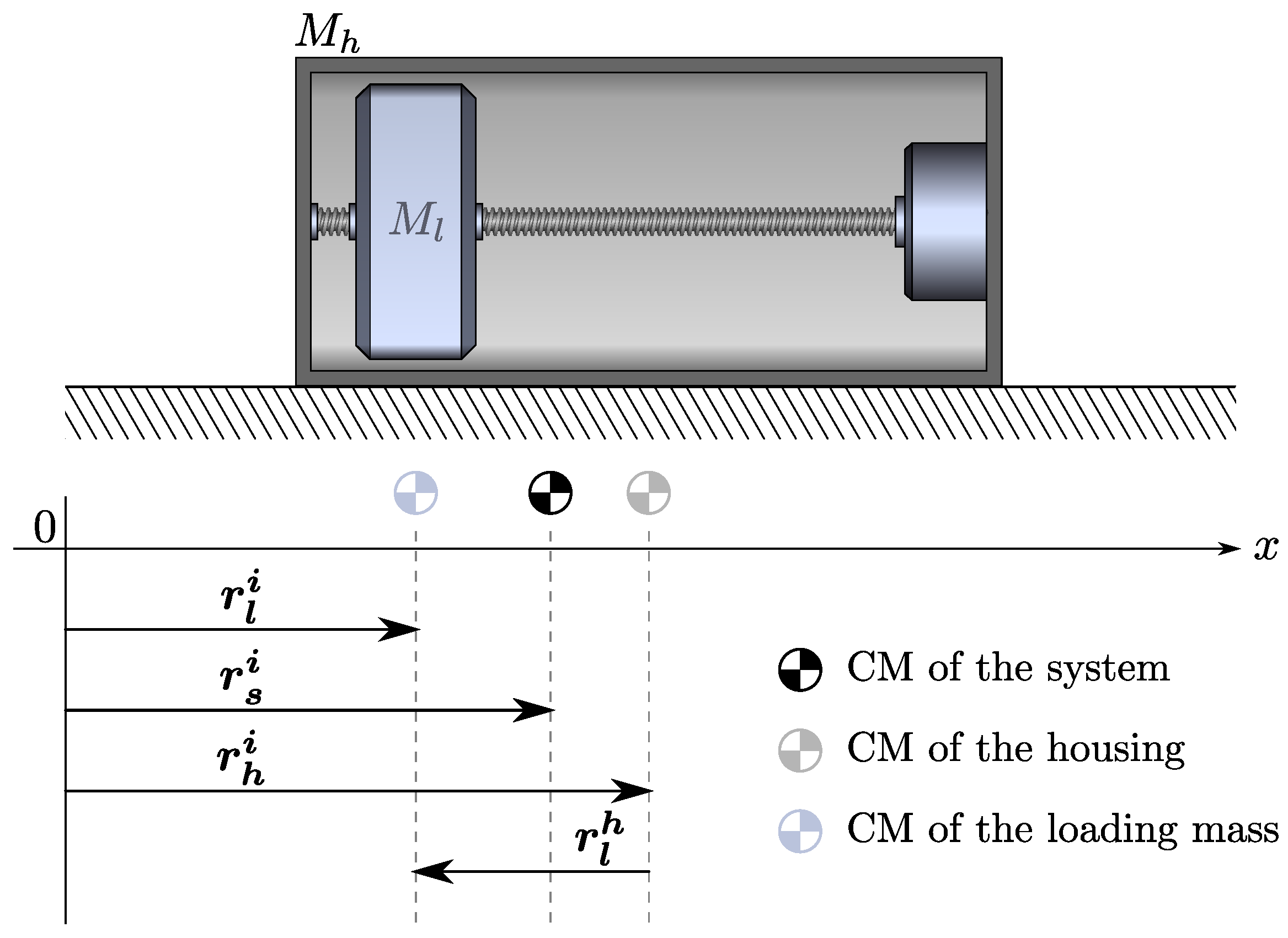
Let us consider the mechanical system shown in Figure 1. It comprises of the loading mass placed within the hollow housing with the mass of . The loading mass can be displaced within the housing along the x axis by a linear actuator. The implementation of the linear actuator itself is not of crucial importance for this conceptual analysis, however, in Figure 1 it is represented by a motor with the shaft connected to a threaded rod that passes through the center of the loading mass. Driving the motor causes the rotation of the threaded rod and displacement of the loading mass along x axis. Both the motor and the rod are connected to the housing and contribute to its mass, . The overall mass of the system is thus . For the sake of simplicity, it is assumed that the system rests in frictionless environment, i.e., there is no friction between the housing and the surface.
Before we start analyzing the system behavior, let us define coordinate frames of interest. The inertial coordinate frame is the outermost frame or the frame of the observer within which the system rests. All vectors expressed within the inertial frame are denoted with “” in superscript. In inertial frame, we define displacement vectors for the center of mass (CM) of the housing, the CM of the loading mass, and the CM of the system, , , and , respectively. The CM of the system is always located between the CM of the housing and the CM of the loading mass. Its position can be calculated as follows:
Multiplying (1) by and differentiating twice with respect to time yields:
Here, , , and represent the accelerations of the system, housing, and loading mass, respectively. Moreover, we can recognize three forces acting on the system and its elements, namely , , and . Notice that the acceleration of the system CM can be caused only by an external force, thus, . The forces and represent the forces acting on the housing and the loading mass, respectively. To understand the relation between these two forces, let us assume for a moment that there is no external force acting on the system (). In this scenario, the total force acting on the housing is equal but opposite to the force acting on the loading mass (). Recall that the force exerted on the loading mass is the driving force caused by the linear actuator. Thus, the force exerted on the housing is the reaction to the actuation the loading mass. In other words, the reaction force is equal but opposite to the driving force (). This is a direct consequence of the conservation of linear momentum principle. Indeed, the total linear momentum of the system, equal to the sum of the housing momentum and the loading mass momentum , is conserved if no external force acts on the system (, being the initial total momentum of the system). In this case, the only forces that appear are the internal forces, which are equal to linear momenta of the system elements differentiated with respect to time ( and ). The initial momentum does not change in time, thus its time derivative is equal to zero (). In general, if there is an external force acting on the system, (3) can be rewritten in terms of the forces acting on the housing:
The total force exerted on the housing is thus equal to the sum of the external force and the reaction force . It is important to notice that the housing experiences an extra push in addition to the external force as a result of driving the loading mass. Furthermore, the total and reaction force acting on the housing can be written as:
Note that the reaction force depends on the acceleration of the loading mass in the inertial frame . Since the loading mass is enclosed within the housing, is difficult to measure directly. However, the displacement of the loading mass within the housing is straightforward to determine. Thus, a new coordinate frame with the origin at the CM of the housing is defined. The displacement of the loading mass is given with vector , as shown in Figure 1. can be expressed as a difference between the displacements of the loading mass and the CM of the housing in inertial frame (see the vectors in Figure 1):
Differentiating (7) twice with respect to time yields the acceleration of the loading mass expressed in the inertial frame.
Now, let us assume that the acceleration of the housing is actively monitored and used to control the acceleration of the loading mass , such that:
Here, k represents an arbitrarily chosen proportionality constant that synchronizes the accelerations and . This synchronization is crucial requirement of the analyzed system. Substituting (9) into (8) yields the relation between and :
Substituting (10) into (6) yields the expression for the reaction force acting on the housing as a function of , k, and :
Finally, substituting the expressions for the total force (5) and the reaction forces (11) acting on the housing and into (4) leads to the following expression:
Equation (12) describes how the housing accelerates in the inertial frame if an external force is applied to it. The proportionality constant between the applied external force and the acceleration of the housing is the effective mass of the system experienced by an external observer.
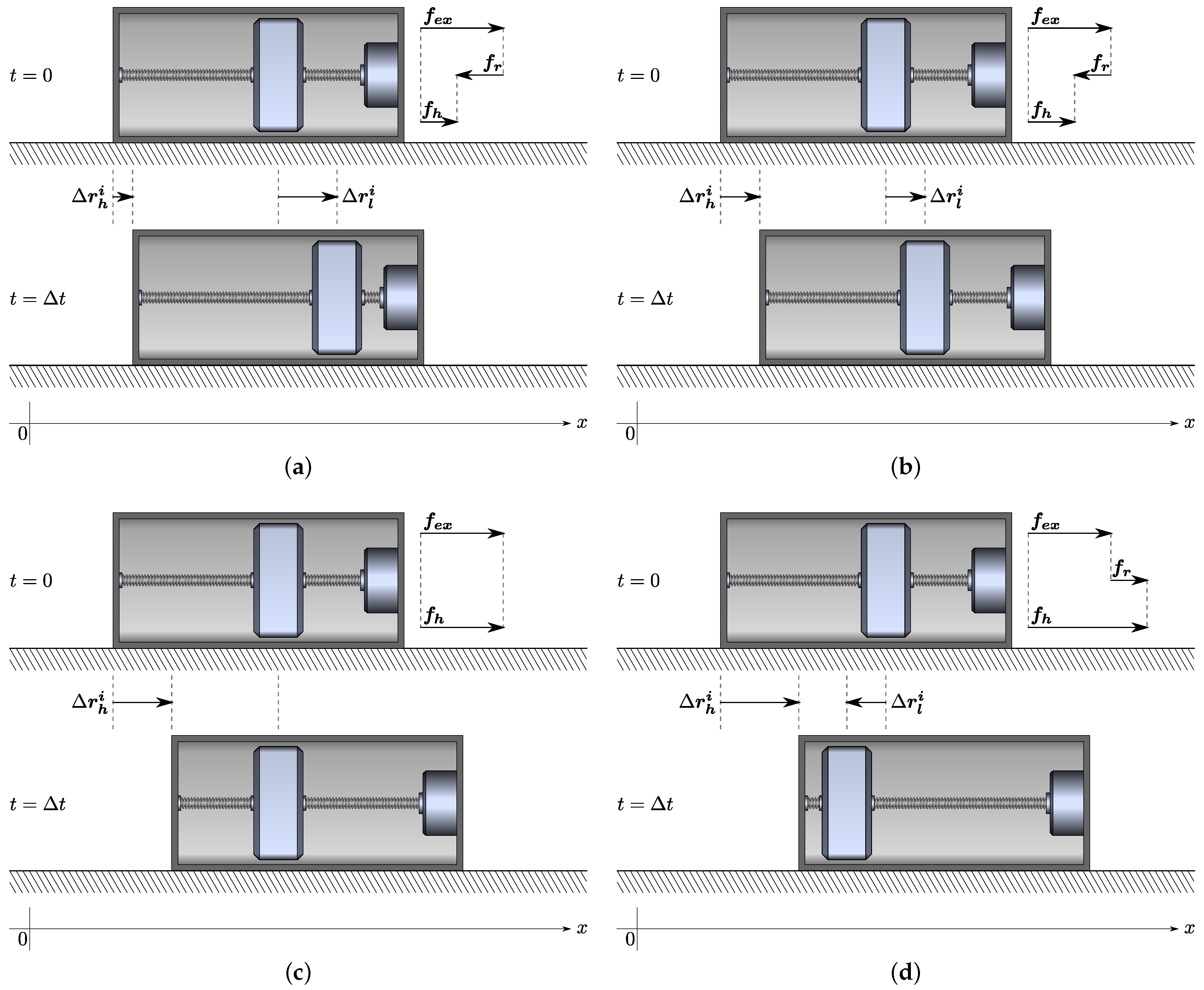
It is important to note that the housing appears as a “black box” to an external observer. In other words, an external observer has no insight into what happens inside the housing. Since the housing experiences two synchronized pushes caused by both the external force and the internal reaction force, its mass effectively appears to be different than for an external observer. As suggested by (13), the correction term depends only on the loading mass and the constant k. To explain this effect in more detail, several examples are given in Figure 2. In all examples it is assumed that the system and all its parts were in the resting state before an external force has been applied (i.e., the velocities of the system and all its parts in inertial frame were equal to zero). The same external force is applied to the system in positive x direction in all examples.
In Figure 2a, the constant k is a positive real number. Because of that, upon the action of the external force, the loading mass accelerates in the housing frame in the same direction as the housing in the inertial frame. The acceleration of the loading mass is caused by the driving force applied by the linear actuator in positive x direction. Such a driving force causes opposite reaction force on the housing, i.e., reaction force in the negative x direction. The reaction force opposes the applied external force reducing the total force exerted on the housing. The reduced total force causes the reduced acceleration of the housing in the inertial frame. Consequently, the effective mass appears larger than the true mass of the system () to an external observer, as suggested by (13). Notice that the relative displacement of the housing is smaller than the relative displacement of the loading mass () after elapsed time .
If (see Figure 2b), there is no motion of the loading mass with respect to the housing. In this example, both the housing and the loading mass accelerate with the same acceleration in inertial frame upon action of the external force, according to (10). In other words, the housing and the loading mass behave as a rigid body with effective mass equal to the sum of the individual masses. Thus, the effective mass seen by an external observer is equal to the mass of the system . The same result is obtained by substituting into (13). In this case the reaction force acts in the same direction as in the previous example; however, its absolute value is smaller, which results in increased total force acting on the housing and reduced effective mass. In this case, the relative displacements of the housing and the loading mass after elapsed time are equal ().
The third example shown in Figure 2c depicts the scenario in which the loading mass accelerates within the housing with the same acceleration as the housing in the inertial frame but in the opposite direction () upon the action of an external force. The acceleration of the loading mass in the inertial frame is equal to zero, as suggested by (10). Since the loading mass was initially in the resting state, it maintains its position in inertial frame even after the force is applied (the displacement vector remains the same, i.e., after elapsed time ). As a result, an external force causes only the acceleration of the housing in the inertial frame. Thus, the effective mass is equal to the mass of the housing , which is exactly the result obtained by substituting into (13). Note that in this example the reaction force vanishes completely. This is not surprising, since the actuation of the loading mass is not required. In a frictionless environment, the loading mass maintains its position due to its own inertia. In reality, this is not completely true. A real-life system would require some level of actuation due to unavoidable friction between the loading mass and the actuator.
Finally, let us consider the fourth example shown in Figure 2d. In this example, k is chosen to be less than . Because of this, the loading mass accelerates in opposite direction with respect to the housing in inertial frame, as suggested by (10). The housing effectively pushes itself from the loading mass, which creates a reaction force in the same direction as the applied external force. In this case, the total force exerted on the housing is larger than the external force, causing larger acceleration of the housing with respect to previous examples. Because of this, the effective mass seen by an external observer drops below , in accordance with (13). As a result of the housing pushing itself from the loading mass, the relative displacement of the loading mass after elapsed time is negative ().
It is important to stress that the CM of the system is displaced by the same distance after the elapsed time in all the examples discussed above, since the same external force is applied. However, the displacement of the CM of the system is not observable by an external observer, but only the displacement of the housing , which manifests its mass depending on k. It is also worth noting that, if , the mass contributed to the effective mass by the correction term is negative (13). In other words, the analyzed mechanical system represents a device able to convert the positive loading mass into its negated and scaled counterpart for , hence the name. Its contribution to the effective mass is equal to the correction term:
If k is chosen such that , then , and the effective mass itself becomes negative (15). This leads to the counterintuitive phenomenon: a negative mass accelerates in the opposite direction to the direction of applied external force. This counterintuitive behavior is the first indication of the system instability, as will be explained later on.
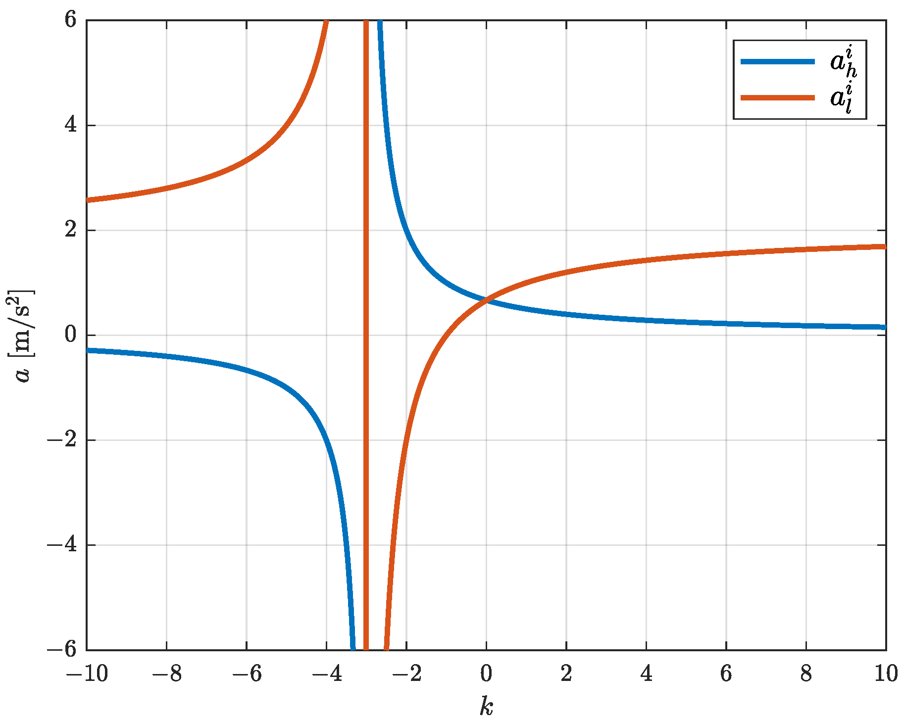
The accelerations of the housing and the loading mass in inertial frame as functions of the parameter k are shown in Figure 3. Here, all the operating points (i.e., specific values of k) examined in the examples described above can be found. In Figure 3, it is assumed that the external force is N and that the masses of the housing and the loading mass are kg and kg, respectively. Since the external force is positive (i.e., the force vector points in the positive x direction), the effective negative mass is achieved for the values of k, for which the acceleration of the housing is negative. Note that producing negative mass requires translation of the loading mass, which certainly requires energy. Although it is not specified in Figure 1, this energy comes from an electric power supply (such as batteries) that is embedded into the housing and contributes to its mass.
2.2. Realization of Negative Moment of Inertia
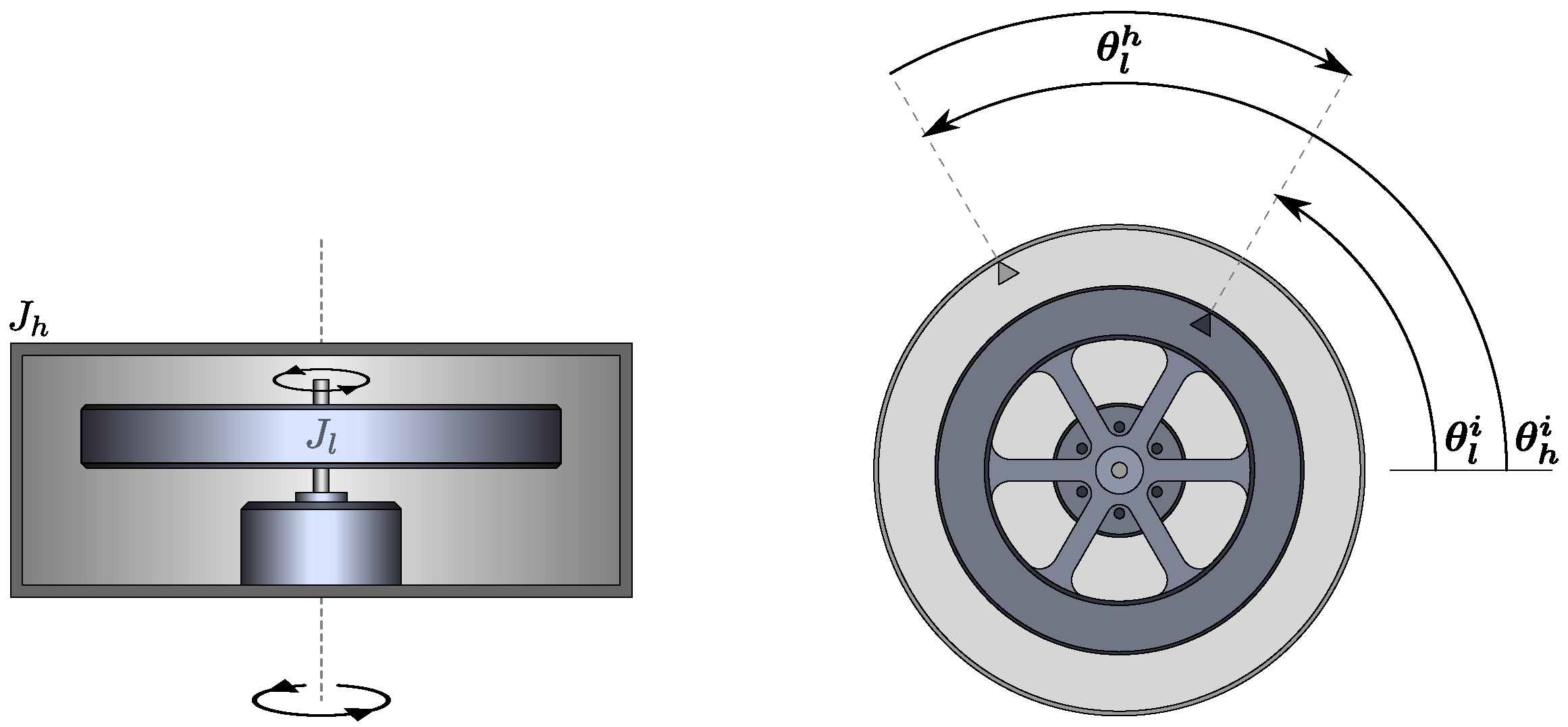
It is quite straightforward to transfer the concepts of translational NICs, examined above in detail, to rotational motion to develop a rotational NIC that is able to produce negative moment of inertia. Such a device is shown in Figure 4. It is composed of a flywheel representing the loading moment of inertia placed within the hollow cylindrical housing with the moment of inertia of . The loading inertia can be rotated within the housing in both clockwise and counterclockwise direction by the motor attached to the housing. The stator of the motor contributes to inertia of the housing , while its rotor contributes to the loading inertia . The overall inertia of the system is thus . Here, again, only the 1D case is analyzed. Furthermore, it is assumed that the system is suspended in a frictionless environment. Since the translational NIC shown in Figure 1 is already examined in detail above, only the key points and equations describing its rotational equivalent shown in Figure 4 are presented here. In these equations the translational quantities (displacement , velocity , and acceleration ) are replaced with the equivalent rotational quantities (angular displacement , angular velocity , and angular acceleration ).
Let us assume that the angular acceleration of the housing expressed in the inertial frame () is monitored and used to control the angular acceleration of the loading inertia with respect to the housing (), such that:
Here, k again represents a real proportionality constant between the two accelerations. Based on (16), the behavior of the rotational NIC can be fully described with the following expressions:
Here, represents the external torque exerted on the system, while and represent the total and the reaction torques exerted on the housing. The reaction torque is a consequence of the conservation of angular momentum and is a result of driving the loading inertia synchronously with the housing, as indicated by (16). The torques and are expressed as functions of moments of inertia and , the angular acceleration of the housing expressed in the inertial frame , and the proportionality constant k. Notice that (17)–(19) are equivalent to (4), (5), and (11) respectively. Substituting (18) and (19) into (17) yields the equation that describes the angular acceleration of the housing upon the action of an external torque:
Notice that for an external observer, the system appears to change its moment of inertia depending on k. The effective moment of inertia observed by an external observer can be written as the sum of the housing and the NIC moments of inertia.
If , the contribution of the NIC to the effective inertia is indeed negative. Moreover, if k is chosen such that , the effective inertia itself becomes negative. Similar to the translational NIC, this again leads to the counterintuitive phenomenon: the angular velocity of a negative moment of inertia increases in opposite direction to the direction of applied external torque. Such a behavior is again an indication of potential system instability.
3. Equivalence of Mechanical and Electrical NICs
The mechanical NICs, described in the previous section, shows many similarities with electrical negative-impedance converters (also abbreviated as NICs) known to the electrical engineering community. Despite the differences in implementation of mechanical and electrical NICs, it can be shown that they are governed by equivalent mathematical models. To prove this statement, let us first introduce the Laplace transforms of mechanical quantities: force, linear velocity, torque, and angular velocity.
Here, , , , and , are functions of complex frequency , where ( represents the imaginary part of complex frequency s and should not to be confused with angular velocity). The relation between and , and and can be found by applying the first derivative property of the Laplace transform [37].
To find the equation equivalent to Equation (24) that describes the relation between electrical quantities current and voltage , let us first define their Laplace transforms.
In the force–current and the torque–current analogy [38], the mathematical equations of the mechanical systems are related to the nodal equations of the electrical system. As a result, torque and force become analogs of current, so as the angular velocity and linear velocity of voltage. To find an electrical analog of mass and moment of inertia, one must look for an electric element that relates the current through the element with the time derivative of the voltage across the element, as indicated by (24). Such an element is a capacitor characterized by its capacitance C.
Comparing (24) and (26) leads to the conclusion that a capacitor is indeed an analog of inertia in mechanical systems. Thus, applying Laplace transform and the force–current analogy to Equations (4), (5), and (11), or the torque–current analogy to Equations (17), (18), and (19), yields a set of equations that describe the electrical equivalents of the mechanical systems. Notice that term represents the admittance of a capacitor, reciprocal to its impedance ().
For better readability, the comparison of all analog quantities of mechanical and electrical NICs, together with the key equations that govern their behavior expressed in Laplace domain, are given in Table 1. The table truly emphasizes the equivalence between the different NICs.
The benefit of the force–current and the torque–current analogy is that Kirchhoff’s current law can be used to develop an equivalent circuit model that has the same topology as the real system. The circuit model drown directly from Equation (27) is shown in Figure 5.
Using Kirchhoff’s voltage law, the output voltage can be written as the difference between the voltages across and .
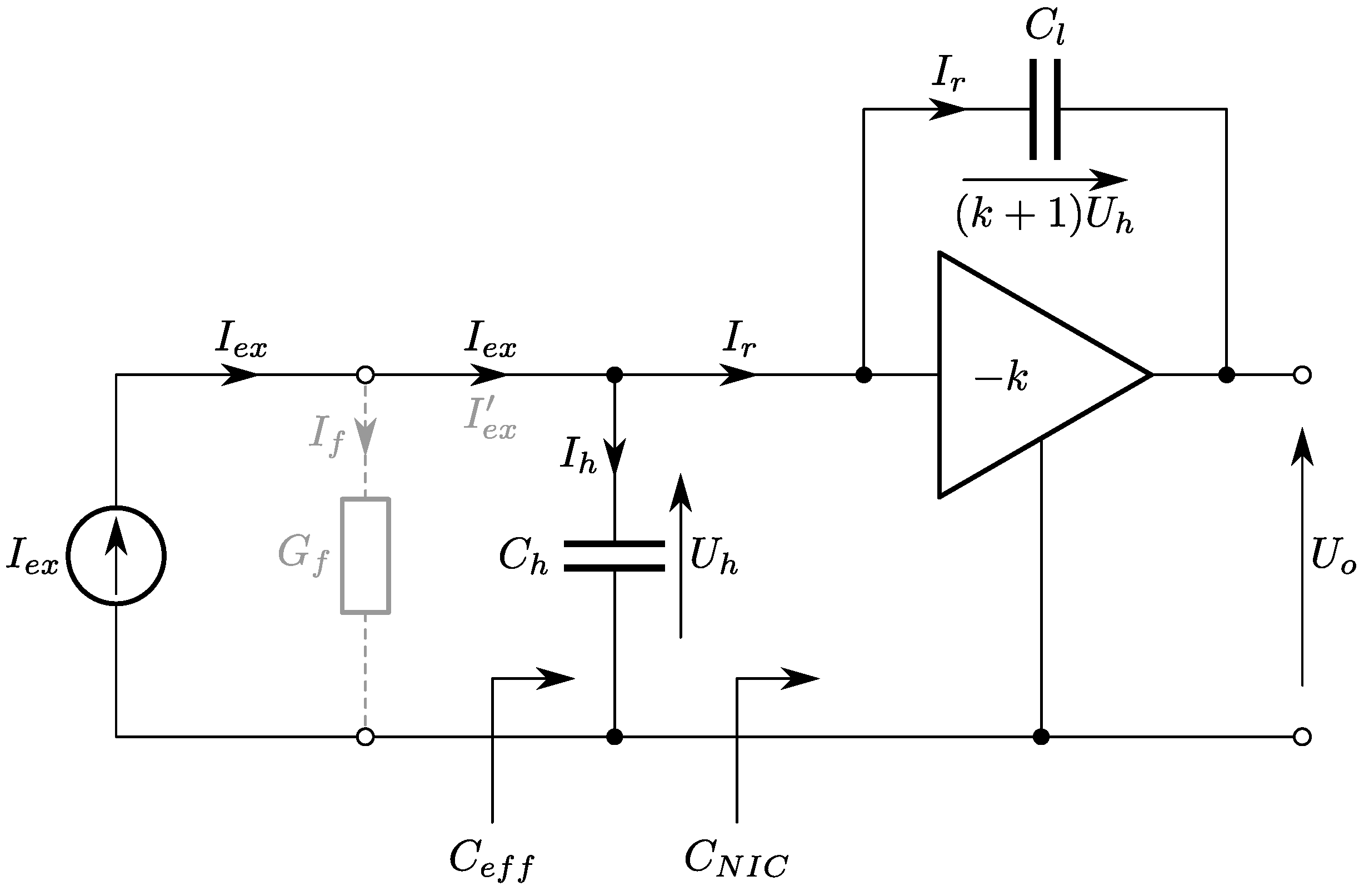
Notice that the voltage represents the voltage multiplied by the factor . This voltage multiplication can be modeled using an ideal inverting voltage amplifier with the constant gain and infinite input impedance. This leads to the final equivalent circuit model shown in Figure 6. For the time being, let us ignore the conductance . It will be important later on.
The input impedance into electrical NIC can be calculated as the ratio between its input voltage and its input current . Thus, we can write:
Equation (29) represents the well-known expression for the input impedance of a NIC expressed as function of the feedback impedance and the gain G. Substituting the expression for the impedance of the capacitor leads to the equivalent NIC capacitance.
Note that if , the inverting amplifier shown in Figure 6 becomes noninverting with the gain . Indeed, an amplifier with the positive feedback loop is a well-known method of a negative-impedance realization. Usually, the amplifier is implemented using an operational amplifier. Such NICs are widely reported in the literature [34,35,36]. In this case, the output voltage of the noninverting amplifier is greater than the input voltage . This causes the current to change its direction increasing the total current through . Furthermore, the capacitance becomes negative for , as suggested by (30b). Since and are in parallel, the equivalent capacitance can be calculated as:
As expected, the expression for the effective capacitance (31) is of the same form as the effective mass (13) and effective moment of inertia (22). This is the final and conclusive proof and confirmation of the equivalence between the three analyzed systems.
4. Simulation Results and Stability Concerns
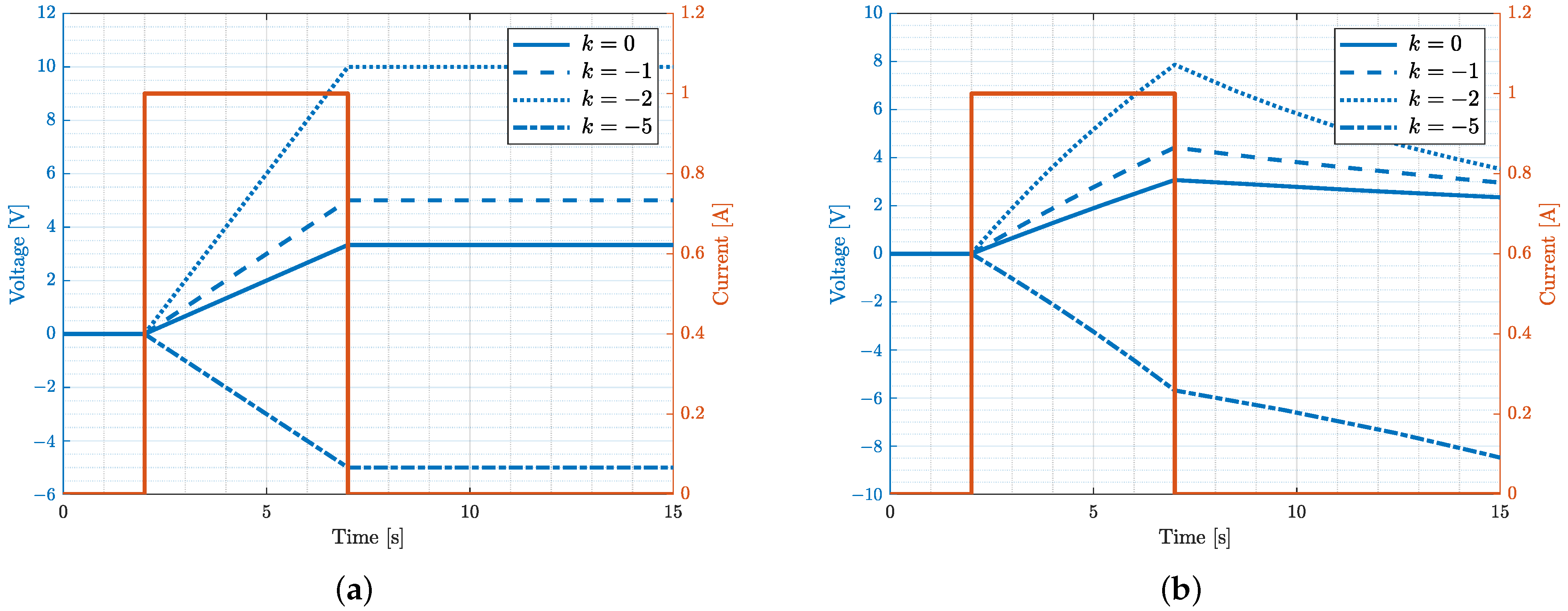
To examine the behavior of the analyzed mechanical NICs, the equivalent circuit model circuit shown in Figure 6 is simulated using LTSpice® circuit simulator by Analog Devices, Inc. The results of the simulations are shown in Figure 7. Due to the force–current and the torque–current analogy, all electrical quantities can be easily interpreted in terms of mechanical quantities (all equivalents are presented in Table 1). For example, the blue graphs in Figure 7 represent the voltage (expressed in V) interpreted as linear or angular velocities of the translational and rotational NIC (expressed in m/s and rad/s, respectively). The voltage is the response of the system to the external current pulse with the peak value of A (the red graph) interpreted as the external force or the external torque exerted on the systems (expressed in N or Nm respectively). The values of the capacitors, representing the mass (kg) and moment of inertia (kgm ), are illustratively chosen to be F and F. These analogies are valid throughout the analysis; however, for convenience we focus solely on electrical quantities. Two cases are examined for different values of parameter k: lossless case with the simulation results presented in Figure 7a and lossy case with the simulation results presented in Figure 7b. In both cases it is assumed that the initial voltage is equal to zero.
In the lossless case (Figure 7a), the value of the conductance in Figure 6 is equal to zero. As expected, if the circuit is driven with a constant current source, the voltage across both and increases linearly with time, as suggested by (26). Note that the same voltage appears across the effective capacitance . Thus, the larger the slope of , the lower . Since depends directly on k (31), the slopes of the blue graphs in Figure 7a are also different for different k. Notice that for , the output voltage is equal to zero regardless of the input voltage . Thus, the right terminal of the capacitor connected to the output of the amplifier is grounded, making the capacitor connected in parallel with . Consequently, the effective capacitance is . In case , the amplifier behaves as an ideal voltage follower. Since both the input and the output voltages of the amplifier are the same, there is no difference in electrical potential across the capacitor and thus there is no current . In this case, the input impedance of the NIC is infinite, making (29). Thus, the effective capacitance is equal to . Since is smaller for than for , the slope of the dashed-blue graph is larger than the slope of the solid-blue graph. Further decreasing k to leads to even smaller and larger voltage slope since the capacitance contributed by the NIC becomes negative (). Eventually, itself becomes negative and changes its orientation even though the current excitation remains positive (notice that the voltage is negative for ). In all the examples above, the voltage remains constant after the current pulse. This is not surprising, since there is no lossy element within the system able to dissipate the energy injected by the current source. Such a system can be classified as a marginally stable system.
To introduce losses into the analysis, let us assume that the mechanical NICs experience a frictional force or torque proportional to the velocity of the housing but in the opposite direction. An example of such a friction is the fluid friction, such as air friction or air drag. Although this velocity dependence may be quite complicated, the linear model is usually a good approximation at low speeds and sufficient to demonstrate the stability properties of the introduced NICs. Such a friction can be modeled with the conductance :
The friction effectively reduces the external force or torque exerted on the system. The resultant force, torque, and the equivalent current are thus equal to:
In the equivalent circuit model the conductance is placed in parallel with the current source and , as shown in Figure 6. This changes the relation between the currents, such that:
Equating (33c) and (34), and substituting the expressions for , , , and (see Equations (27), (31), and (32)) leads to the relation between and in the lossy system.
Equation (35) can be used to define the transfer function of the system in Laplace domain. Indeed, if is treated as the system output and as the system input, the transfer function is the ratio between the two.
Notice that the analyzed system is a first-order system with a single pole , defined by the root of the transfer function denominator, placed at the real axis of the complex plane ():
The location of the pole in complex plane is consistent with the poles of the similar systems reported in the literature [39,40]. It is associated with the characteristic time-domain exponential response of the form , where represents the time constant (not to be confused with torque). These exponential responses can be seen clearly in Figure 7b. During the current pulse, increases exponentially in contrast to the linear voltage increase seen in Figure 7a. After the current pulse, discharges on , causing exponential decrease of the voltage also related to the time constant . Recall that in lossless case the voltage remains constant after the current pulse. It is important to notice that for , the voltage exponentially drops to zero with time. However, for after the current pulse, the voltage keeps decreasing exponentially to . Such an unbounded exponential response is characteristic of unstable systems. Indeed, is negative for , making the time constant negative. In general, a system is unstable if one of its poles is placed in the right half-plane of the complex plane. Thus, to ensure the system stability, all the system poles must be located within the left half-plane, i.e., the real part of all the system poles must be negative. Applying this criterion to the analyzed system leads to the conclusion that the system pole must be negative. Since is a positive real number, this criterion is met only if:
The inequality (38) represents the stability condition of the system shown in Figure 6. If, however, the system is lossless (), the pole is located at the origin of the complex plane () regardless of . Such a system is not stable nor unstable, but rather at the stability margin, which validates the classification of the lossless system as marginally stable. The stability condition (38) is easily applied to the mechanical NICs: in order to be stable, the effective mass or effective moment of inertia must be positive.
Stability is the crucial requirement of every practical system, with the exception of some very specialized systems such as oscillators. The instability provides an explanation of why negative inertia is such a counterintuitive concept. Negative inertia in not observable in everyday life since it would be unstable. In other words, such a system requires infinite energy and thus it is unsustainable in the common physical setup that we are accustomed to.
5. Applications and Limitations of Negative-Inertia Converters
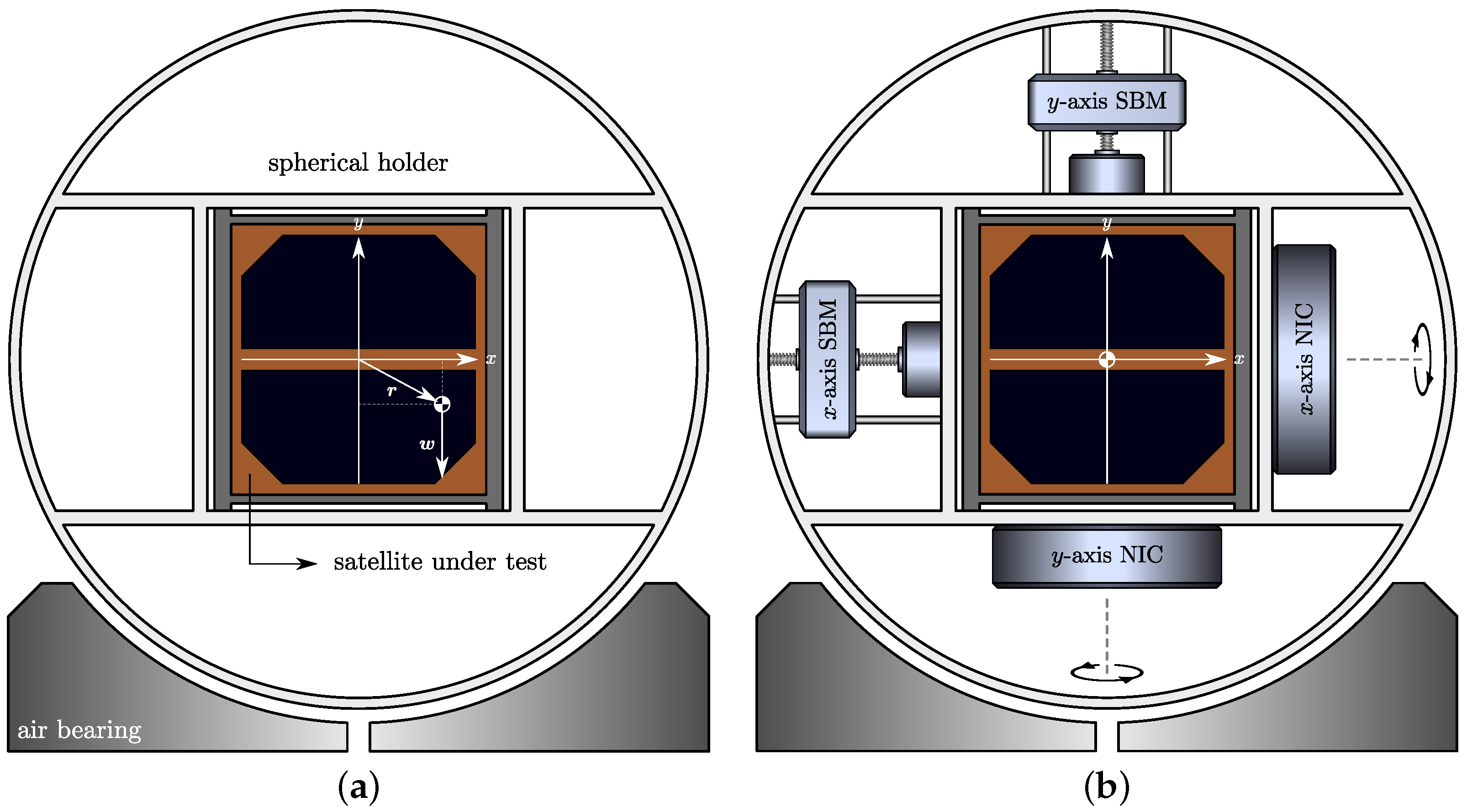
Although the stability criterion is the limiting factor in the design of systems based on mechanical NICs, they may still find their applications in many fields. The most obvious application is the reduction of an object’s inertia. Indeed, if a translational NIC is attached to another object, is increased by the mass of the object, which allows even lower values of k to be chosen (). This fact allows full reduction of and partial reduction of the mass of the object, while keeping . The same concept can be applied to rotational systems with the rotational NIC. The inertia reduction may be especially important in measurement setups in which the inertia of the setup interferes with the measurements or is difficult to eliminate in postprocessing. An example of such a measurement setup is an attitude determination and control system testbed for validation of nanosatellites in laboratory conditions prior to launch into orbit. An example of such a setup is shown in Figure 8. The purpose of the testbed is to emulate conditions that a satellite experiences in orbit, the most important of which are frictionless and weightless state. To eliminate friction, the satellite under test is placed within the spherical holder of the same radius as the spherical air bearing. A thin film of compressed air fed from an air compressor is created between the spherical holder and air bearing separating one from another and eliminating the friction between them. A weightless state is achieved by adjusting the center of mass of the spherical holder and all its components along orthogonal axes by using sliding balancing masses (SBM) such that the center of mass coincides with the center of rotation located at the geometric center of the spherical holder. In such a way, the unwonted gravitational torque ( and being the displacement vector and the weight of the setup respectively) is eliminated and all three degrees of rotational freedom ensured. However, the SBMs introduce additional mass to the system and increase the overall moment of inertia. As a consequence, the satellite dynamics in laboratory conditions deviate from the dynamics in orbit, complicating the testing and optimization of the satellite. The solution to this problem lies in rotational NICs. By using rotational NICs, the unwonted moment of inertia introduced by the testbed itself can be fully eliminated while maintaining the effective moment of inertia equal to the moment of inertia of the satellite under test. Since remains positive, the condition (39b) is satisfied and stability is ensured. Although attempts of active moment of inertia compensation of the satellite testbed have been reported [41], to the best of the authors’ knowledge, the proposed approach is the first self-consisted method that does not require prior knowledge of the satellite’s dynamics and mechanical properties.
The translational and rotational NICs undoubtedly manifest quite interesting properties, however, one should be aware of their limitations. For example, the translational NIC has a displacement range of the loading mass limited by the size of the housing, since it is enclosed by the housing. Such an NIC is suitable for applications that do not require a wide actuation range. These applications may imply periodic or oscillatory translational motion of the NIC housing and loading mass. For example, the translational NIC is suitable for mass reduction with the goal of increasing the resonant frequency of a mechanical setup. The challenge of a limited actuation range can be mitigated by increasing , which decreases the value of k and displacement of the loading mass within the housing for the same . Furthermore, it may be possible to apply the same principles to systems with loading masses not confined within the housings, which would increase the actuation range of the NIC. Examples of such systems include a bullet (the loading mass) inside of a gun (the housing) and rocket fuel (the loading mass) inside a fuel tank (the housing). In contrast to the translational NIC, the actuation range of the rotational NIC is not limited. This makes it highly practical even for longer lasting external torques. However, one should be aware that a constant external torque causes constant angular acceleration of the housing and, thus, constant angular acceleration of the loading inertia, which eventually drives the motor into a nonlinear saturated mode. In other words, the actuation of the loading mass is limited by the maximal angular velocity of the motor. The same applies to the translational NIC and any real-life system. Indeed, no real-life system is perfectly linear.
6. Conclusions
In this paper, novel concepts of negative-inertia converters for both translational and rotational motion are introduced. The proposed devices are capable of obtaining negative mass and negative moment of inertia by synchronous actuation of the loading inertia with the acceleration of the housing. Negative-inertia converters share many similarities with electrical negative-impedance converters, including their proneness to instability. It is found that friction can cause a counterintuitive unbounded exponential response, indicating the system’s instability. The derived closed-form stability condition suggests that the effective inertia must be positive to ensure the stability of the system. Although the instability is a limiting factor, negative-inertia converters may become the key elements in applications requiring the reduction of an object’s inertia. The presented one-dimensional converters can be easily generalized to all three spatial dimensions by using three orthogonally oriented NICs. Since all three orthogonal converters are controlled independently, designing a system with an arbitrary value of inertia along each orthogonal axis is feasible. While it is not surprising that nonsymmetrical objects manifest different moments of inertia for rotation around different coordinate axes, to the best of the authors’ knowledge, similar manifestation of the object’s mass has not been reported. The experimental verification of the presented concepts and underlying theory will be the subject of our future research efforts.
Author Contributions
Conceptualization, J.L.; methodology, J.L.; software, J.L.; validation, B.I.; formal analysis, J.L., B.I.; investigation, J.L., B.I.; resources, J.L.; writing—original draft preparation, J.L.; writing—review and editing, J.L., B.I., D.B.; visualization, J.L.; funding acquisition, D.B. All authors have read and agreed to the published version of the manuscript.
Funding
This research has been supported by the European Regional Development Fund under the grant KK.01.1.1.01.0009 (DATACROSS).
Conflicts of Interest
The authors declare no conflict of interest.
References
- Bilotti, F.; Sevgi, L. Metamaterials: Definitions, properties, applications, and FDTD-based modeling and simulation. Int. J. Microw.-Comput.-Aided Eng. 2012, 22, 422–438. [Google Scholar] [CrossRef]
- Tretyakov, S.A. A personal view on the origins and developments of the metamaterial concept. J. Opt. 2016, 19, 013002. [Google Scholar] [CrossRef]
- Veselago, V.G. The electrodynamics of substances with simultaneously negative values of e and u. Sov. Phys. Usp. 1968, 10, 509–514. [Google Scholar] [CrossRef]
- Tierney, B.B.; Grbic, A. Designing anisotropic, inhomogeneous metamaterial devices through optimization. IEEE Trans. Antennas Propag. 2018, 67, 998–1009. [Google Scholar] [CrossRef]
- Sarabandi, K.; Behdad, N. A frequency selective surface with miniaturized elements. IEEE Trans. Antennas Propag. 2007, 55, 1239–1245. [Google Scholar] [CrossRef]
- Pfeiffer, C.; Grbic, A. Millimeter-wave transmitarrays for wavefront and polarization control. IEEE Trans. Microw. Theory Tech. 2013, 61, 4407–4417. [Google Scholar] [CrossRef]
- Lončar, J.; Grbic, A.; Hrabar, S. Ultrathin active polarization-selective metasurface at X-band frequencies. Phys. Rev. B 2019, 100, 075131. [Google Scholar] [CrossRef]
- Liu, J.; Guo, H.; Wang, T. A review of acoustic metamaterials and phononic crystals. Crystals 2020, 10, 305. [Google Scholar] [CrossRef]
- Li, Z.; Wang, C.; Wang, X. Modelling of elastic metamaterials with negative mass and modulus based on translational resonance. Int. J. Solids Struct. 2019, 162, 271–284. [Google Scholar] [CrossRef]
- Graciá-Salgado, R.; García-Chocano, V.M.; Torrent, D.; Sánchez-Dehesa, J. Negative mass density and ρ-near-zero quasi-two-dimensional metamaterials: Design and applications. Phys. Rev. B 2013, 88, 224305. [Google Scholar] [CrossRef]
- Bormashenko, E.; Legchenkova, I. Negative effective mass in plasmonic systems. Materials 2020, 13, 1890. [Google Scholar] [CrossRef] [PubMed] [Green Version]
- Barchiesi, E.; Di Cosmo, F.; Laudato, M. A review of some selected examples of mechanical and acoustic metamaterials. Discret. Contin. Model. Complex Metamater. 2020, 2020, 52–102. [Google Scholar]
- Khamehchi, M.; Hossain, K.; Mossman, M.; Zhang, Y.; Busch, T.; Forbes, M.M.; Engels, P. Negative-mass hydrodynamics in a spin-orbit–coupled bose-einstein condensate. Phys. Rev. Lett. 2017, 118, 155301. [Google Scholar] [CrossRef] [PubMed]
- Colas, D.; Laussy, F.P.; Davis, M.J. Negative-mass effects in spin-orbit coupled Bose-Einstein condensates. Phys. Rev. Lett. 2018, 121, 055302. [Google Scholar] [CrossRef] [Green Version]
- Alcubierre, M. The warp drive: Hyper-fast travel within general relativity. Class. Quantum Gravity 1994, 11, L73. [Google Scholar] [CrossRef]
- Farnes, J.S. A unifying theory of dark energy and dark matter: Negative masses and matter creation within a modified ΛCDM framework. Astron. Astrophys. 2018, 620, A92. [Google Scholar] [CrossRef] [Green Version]
- Yang, L.; Wang, L. An ultrawide-zero-frequency bandgap metamaterial with negative moment of inertia and stiffness. New J. Phys. 2021, 23, 043003. [Google Scholar] [CrossRef]
- Foster, R.M. A Reactance Theorem. Bell Labs Tech. J. 1924, 3, 259–267. [Google Scholar] [CrossRef]
- Merrill, J., Jr. Theory of the negative impedance converter. Bell Syst. Tech. J. 1951, 30, 88–109. [Google Scholar] [CrossRef]
- Sievenpiper, D.F. Superluminal Waveguides Based on Non-Foster Circuits for Broadband Leaky-wave Antennas. IEEE Antennas Wirel. Propag. Lett. 2011, 10, 231–234. [Google Scholar] [CrossRef]
- Weldon, T.P.; Miehle, K.; Adams, R.S.; Daneshvar, K. A Wideband Microwave Double-negative Metamaterial with Non-Foster Loading. In Proceedings of the 2012 IEEE Southeastcon, Orlando, FL, USA, 15–18 March 2012; pp. 1–5. [Google Scholar]
- Linvill, J.G. Transistor Negative Impedance Converters. Proc. IRE 1953, 41, 725–729. [Google Scholar] [CrossRef]
- Linvill, J.G. RC Active Ffilters. Proc. IRE 1954, 42, 555–564. [Google Scholar] [CrossRef]
- Larky, A. Negative-impedance Converters. IRE Trans. Circuit Theory 1957, 4, 124–131. [Google Scholar] [CrossRef]
- Gao, F.; Zhang, F.; Long, J.; Jacob, M.; Sievenpiper, D. Non-dispersive Tunable Reflection Phase Shifter Based on Non-Foster Circuits. Electron. Lett. 2014, 50, 1616–1618. [Google Scholar] [CrossRef]
- Perry, A.K. Broadband Antenna Systems Realized from Active Circuit Conjugate Impedance Matching; Technical Report, DTIC Document; Naval Postgraduate School: Monterey, CA, USA, 1973; Available online: https://apps.dtic.mil/sti/citations/AD0769800 (accessed on 25 January 2022).
- Song, K.S.; Rojas, R.G. Electrically Small Wire Monopole Antenna with Non-Foster Impedance Element. In Proceedings of the IEEE Fourth European Conference on Antennas and Propagation, Barcelona, Spain, 12–16 April 2010; pp. 1–4. [Google Scholar]
- Zhu, N.; Ziolkowski, R.W. Design and Measurements of an Electrically Small, Broad Bandwidth, Non-Foster Circuit-augmented Protractor Antenna. Appl. Phys. Lett. 2012, 101, 024107. [Google Scholar] [CrossRef] [Green Version]
- Jacob, M.M.; Long, J.; Sievenpiper, D.F. Broadband Non-Foster Matching of an Electrically Small Loop Antenna. In Proceedings of the IEEE International Symposium on Antennas and Propagation Society (APSURSI), Chicago, IL, USA, 8–14 July 2012; pp. 1–2. [Google Scholar]
- Almokdad, S.; Lababidi, R.; Le Roy, M.; Sadek, S.; Pérennec, A.; Le Jeune, D. Methodology for broadband matching of electrically small antenna using combined non-Foster and passive networks. Analog. Integr. Circuits Signal Process. 2020, 104, 251–263. [Google Scholar] [CrossRef]
- Xia, Y.; Li, Y.; Zhang, S. A non-foster matching circuit for an ultra-wideband electrically small monopole antenna. In Proceedings of the IEEE 13th European Conference on Antennas and Propagation, Krakow, Poland, 31 March–5 April 2019; pp. 1–3. [Google Scholar]
- Ghadiri, A.; Moez, K. Gain-enhanced Distributed Amplifier Using Negative Capacitance. IEEE Trans. Circuits Syst. Regul. Pap. 2010, 57, 2834–2843. [Google Scholar] [CrossRef]
- Lončar, J.; Šipuš, Z. Challenges in design of power-amplifying active metasurfaces. In Proceedings of the 2020 IEEE International Symposium ELMAR, Zadar, Croatia, 14–15 September 2020; pp. 9–12. [Google Scholar]
- Lončar, J.; Grbic, A.; Šipuš, Z. Synthesis of NIC-based Reflection Amplifiers for Metasurfaces. In Proceedings of the 2020 IEEE Fourteenth International Congress on Artificial Materials for Novel Wave Phenomena (Metamaterials), New York, NY, USA, 27 September–3 October 2020; pp. 456–458. [Google Scholar]
- Lončar, J.; Hrabar, S. Stability of metasurface-based parity-time symmetric systems. In Proceedings of the 2016 IEEE 10th International Congress on Advanced Electromagnetic Materials in Microwaves and Optics (METAMATERIALS), Chania, Greece, 19–22 September 2016; pp. 130–132. [Google Scholar]
- Lončar, J.; Vuković, J.; Krois, I.; Hrabar, S. Stability Constraints on Practical Implementation of Parity-Time-Symmetric Electromagnetic Systems. Photonics 2021, 8, 56. [Google Scholar] [CrossRef]
- Bellman, R.; Roth, R.S. The Laplace Transform; World Scientific: Singapore, 1984; Volume 3. [Google Scholar]
- Firestone, F.A. A new analogy between mechanical and electrical systems. J. Acoust. Soc. Am. 1933, 4, 249–267. [Google Scholar] [CrossRef] [Green Version]
- Lončar, J.; Muha, D.; Hrabar, S. Influence of transmission line on stability of networks containing ideal negative capacitors. In Proceedings of the 2015 IEEE International Symposium on Antennas and Propagation & USNC/URSI National Radio Science Meeting, Vancouver, BC, Canada, 19–24 July 2015; pp. 73–74. [Google Scholar]
- Lončar, J.; Hrabar, S.; Muha, D. Stability of Simple Lumped-distributed Networks with Negative Capacitors. IEEE Trans. Antennas Propag. 2016, 65, 390–395. [Google Scholar] [CrossRef]
- Gavrilovich, I.; Krut, S.; Gouttefarde, M.; Pierrot, F.; Dusseau, L. Test bench for nanosatellite attitude determination and control system ground tests. In Proceedings of the 4S: Small Satellites Systems and Services Symposium, Majorca, Spain, 26–30 May 2014; ESA: Noordwijk, The Netherlands, 2014. [Google Scholar]
Figure 1.
Implementation of a negative-inertia converter designed for translational motion. The NIC consists of a loading mass confined within a housing with the mass of . The loading mass can be displaced along the x axis using the linear actuator based on the threaded rod and the motor attached to the housing.

Figure 2.
Examples of the housing and the loading mass displacements for different values of k upon action of the same external force. The total force acting on the housing , equal to the sum of the external force and the reaction force , is depicted qualitatively. (a) k > 0, (b) , (c) , (d) k < −1.

Figure 3.
Acceleration of the housing (kg) and the loading mass (kg) in the inertial frame of reference upon the action of a constant external force (N).
Figure 3.
Acceleration of the housing (kg) and the loading mass (kg) in the inertial frame of reference upon the action of a constant external force (N).

Figure 4.
Side view (left) and top view (right) of a rotational NIC. It consists of a flywheel with the loading moment of inertia confined within a housing with the moment of inertia of . The flywheel can be rotated both in clockwise and counterclockwise direction.
Figure 4.
Side view (left) and top view (right) of a rotational NIC. It consists of a flywheel with the loading moment of inertia confined within a housing with the moment of inertia of . The flywheel can be rotated both in clockwise and counterclockwise direction.

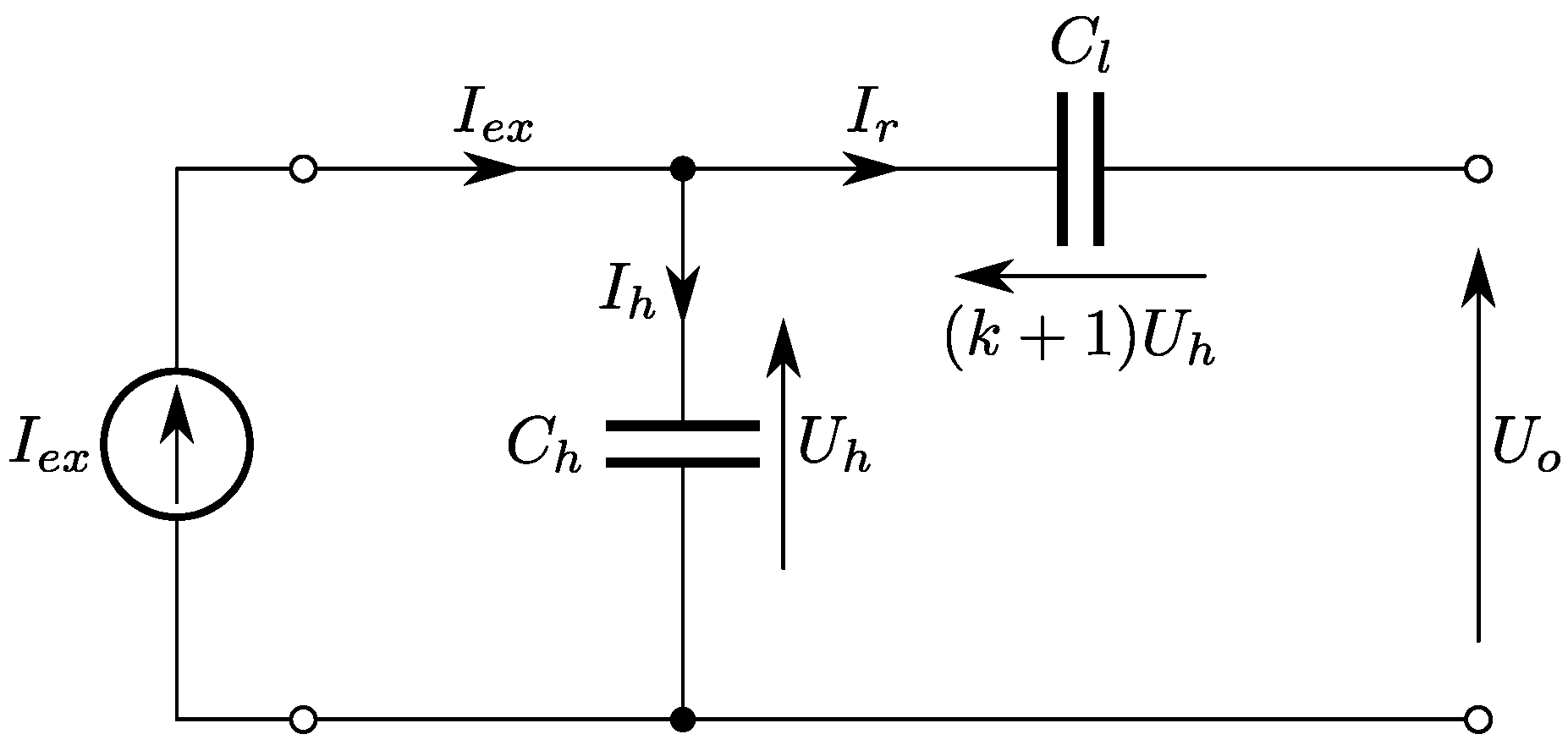
Figure 5.
Equivalent circuit model of the mechanical systems shown in Figure 1 and Figure 4 based on equations Equation (27).

Figure 6.
Equivalent circuit model of the mechanical systems shown in Figure 1 and Figure 4 based on the electrical NIC circuitry.

Figure 7.
Simulation results of the equivalent circuit model shown in Figure 6. The graphs show voltage (blue curves) for different k. The system is excited by the external current source (red curve). The capacitance values are illustratively chosen to be F and F. (a) Lossless system (). (b) System with losses (S).

Figure 8.
Uncompensated CubeSat testbed (a) with the center of mass displaced from the center of rotation, and the compensated testbed (b) with balanced mass and compensated moments of inertia.
Figure 8.
Uncompensated CubeSat testbed (a) with the center of mass displaced from the center of rotation, and the compensated testbed (b) with balanced mass and compensated moments of inertia.


Table 1.
Comparison of the analog quantities and equations of mechanical and electrical NICs expressed in Laplace domain.
Table 1.
Comparison of the analog quantities and equations of mechanical and electrical NICs expressed in Laplace domain.
| Translational NIC | Rotational NIC | Electrical NIC | |||
|---|---|---|---|---|---|
| Description | Expression | Description | Expression | Description | Expression |
| Mass | M | Moment of inertia | J | Capacitance | C |
| Linear Velocity | Angular Velocity | Voltage | U | ||
| Force | Torque | Current | I | ||
| Total Force | Total Torque | Total Current | |||
| Reaction Force | Reaction Torque | Reaction Current | |||
| External Force | External Torque | External Current | |||
Publisher’s Note: MDPI stays neutral with regard to jurisdictional claims in published maps and institutional affiliations. |
© 2022 by the authors. Licensee MDPI, Basel, Switzerland. This article is an open access article distributed under the terms and conditions of the Creative Commons Attribution (CC BY) license (https://creativecommons.org/licenses/by/4.0/).
Share and Cite
MDPI and ACS Style
Lončar, J.; Igrec, B.; Babić, D. Negative-Inertia Converters: Devices Manifesting Negative Mass and Negative Moment of Inertia. Symmetry 2022, 14, 529. https://0-doi-org.brum.beds.ac.uk/10.3390/sym14030529
AMA Style
Lončar J, Igrec B, Babić D. Negative-Inertia Converters: Devices Manifesting Negative Mass and Negative Moment of Inertia. Symmetry. 2022; 14(3):529. https://0-doi-org.brum.beds.ac.uk/10.3390/sym14030529
Chicago/Turabian StyleLončar, Josip, Bojan Igrec, and Dubravko Babić. 2022. "Negative-Inertia Converters: Devices Manifesting Negative Mass and Negative Moment of Inertia" Symmetry 14, no. 3: 529. https://0-doi-org.brum.beds.ac.uk/10.3390/sym14030529
Note that from the first issue of 2016, this journal uses article numbers instead of page numbers. See further details here.