Impact of Brownian Motion on the Analytical Solutions of the Space-Fractional Stochastic Approximate Long Water Wave Equation

Abstract

The space-fractional stochastic approximate long water wave equation (SFSALWWE) is considered in this work. The Riccati equation method is used to get analytical solutions of the SFSALWWE. This equation has never been examined with stochastic term and fractional space at the same time. In general, the noise term that preserves the symmetry reduces the domain of instability. To check the impact of Brownian motion on these solutions, we use a MATLAB package to plot 3D and 2D graphs for some analytical fractional stochastic solutions.

1. Introduction

Stochastic differential equations (SDEs) are extremely suitable for representing a wide range of physical phenomena in various fields such as biology, chemistry, physics, engineering, oceanography, environmental sciences, etc. [1,2,3]. SDEs are particularly important in explaining all dynamical systems in which particle-physics influences are either ignored or recognized perturbations. They could be considered as an extension of dynamical systems theory to models with noise. This external stochastic effect is always present in real systems because they cannot be completely isolated from their surroundings.

From another perspective, fractional derivatives are utilized to characterize numerous physical phenomena in mathematical biology, engineering applications, electromagnetic theory, signal processing, and different scientific studies. For example, the fractional derivative is used throughout the fields of signal processing, viscoelasticity, control theory, optics, dynamical system, controller tuning, and seismic wave analysis. Many articles are published about certain attributes of fractional partial differential equations (FPDEs), such as techniques for solution stability, the uniqueness and existence of solutions, and numerical and exact solutions [4,5,6,7,8,9]. Recently, much time and effort have gone into developing exact solutions for FPDEs, and many strong methods have been created for instance-modified trial equation, exp-function, $(G^{\prime }/G)$-expansion, sine–cosine, Jacobi elliptic function, modified trial equation, tanh–sech, and modified Kudryashov Methods [10,11,12,13,14,15,16,17,18,19,20,21,22].

A few articles, such as [23,24,25,26,27], have investigated the acquired exact solutions for fractional SDEs. As a result, we treat here the following space-fractional stochastic approximate long water wave equation (SFSALWWE) with multiplicative noise:

$$\begin{array}{ccc}\hfill d\phi +[\frac{1}{2}{\mathcal{D}}_y^{2\alpha }\phi -\phi {\mathcal{D}}_y^{\alpha }\phi -{\mathcal{D}}_y^{\alpha }\psi ]dt& =& \rho \phi d\beta \hfill \end{array}$$

(1)

$$\begin{array}{ccc}\hfill d\psi -[{\mathcal{D}}_y^{\alpha }\left(\phi \psi \right)+\frac{1}{2}{\mathcal{D}}_y^{2\alpha }\psi ]dt& =& \rho \psi d\beta ,\hfill \end{array}$$

(2)

where ${\mathcal{D}}^{\alpha }$ is the conformable fractional derivative (CFD) [28], $\rho$ is a noise intensity, $\beta \left(t\right)$ is the Brownian motion, and $\phi d\beta$ and $\psi d\beta$ are multiplicative noise in the Itô sense.

Many researchers have acquired the precise solutions of SFSALWWE (Equations (1) and (2)) with $\alpha =1$ and $\rho =0$ by utilizing different techniques, including the $(G^{\prime }/G)$-expansion method [29], improved $(G^{\prime }/G)$-expansion [30], and generalized extended tanh-function [31]. Moreover, the fractional deterministic approximate long water wave equation (i.e., Equations (1) and (2) with $\rho =0$) has been solved via various methods, such as $eyp(-\varphi (\varsigma \left)\right)$-expansion [32,33], the fractional sub-equation [34], $(G^{\prime }/G)$-expansion [35], and generalized Kudryashov [36].

Our aim here is to utilise the Riccati equation method to secure the exact fractional-stochastic solutions of the SFSALWWE (Equations (1) and (2)) since the exact solutions of the stochastic approximate long water wave equation have not been studied. Hence, the novelty of this article is to obtain exact solutions to such equations. The effects of multiplicative noise on these solutions are also looked into, and we deduce that t he noise term that preserves the symmetry stabilizes the obtained solutions. This is the first publication to discover the exact solution to the SFSALWWE (Equations (1) and (2)) by using a conformable fractional derivative.

The following is how this article will be structured: In the next section, we define and declare the features of CFD. In Section 3, the wave equation for the SFSALWWE (Equations (1) and (2)) is obtained, while in Section 4, we use the Riccati equation method to attain the analytical stochastic solutions of the SFSALWWE (Equations (1) and (2)). In Section 5, we exhibit multiple graphs to clarify the effect of multiplicative noise on SFSALWWE solutions. In Section 6, we present the physical interpretation of our results. In the end, we introduce the paper’s conclusions.

2. Conformable Derivative and Its Properties

We discuss here the basic definition, theorem, and properties of a CFD [28].

Definition 1.

Let $f:(0,\infty )\to \mathbb{R}$, then the CFD of f of order α is defined as

$${\mathbb{T}}_y^{\alpha }f\left(y\right)=\underset{h\to 0}{lim}\frac{f(y+h{y}^{1-\alpha })-f\left(y\right)}{h}.$$

Theorem 1.

Let $f,g:(0,\infty )\to \mathbb{R}$ be differentiable, and also α differentiable functions, then the next rule holds:

$${\mathbb{T}}_y^{\alpha }(f\circ g)\left(y\right)=y^{1-\alpha }{g}^{\prime }\left(y\right)f^{\prime }\left(g\left(y\right)\right).$$

Let us state some properties of the CFD:

• ${\mathcal{D}}_y^{\alpha }[af\left(y\right)+\ell g\left(y\right)]=a{\mathcal{D}}_y^{\alpha }f\left(y\right)+\ell {\mathcal{D}}_y^{\alpha }g\left(y\right),a,\ell \in \mathbb{R}$
• ${\mathcal{D}}_y^{\alpha }\left[C\right]=0,C$ is a constant
• ${\mathcal{D}}_y^{\alpha }\left[y^{\gamma }\right]=\gamma y^{\gamma -\alpha },\gamma \in \mathbb{R}$
• ${\mathcal{D}}_y^{\alpha }g\left(y\right)=y^{1-\alpha }\frac{dg}{dy}$

3. Wave Equation for SFSALWWE

We take the wave transformation

$$\phi (y,t)=u\left(\eta \right)e^{(\rho \beta \left(t\right)-\frac{1}{2}{\rho }^{2}t)},\psi (y,t)=v{e}^{(\rho \beta \left(t\right)-\frac{1}{2}{\rho }^{2}t)},\eta =\frac{1}{\alpha }{y}^{\alpha }+\omega t,$$

(3)

in order to get the wave equation of SFSALWWE (Equations (1) and (2)). Where u and v are deterministic functions and $\omega$ is a constant. Substituting Equation (3) into Equations (1) and (2) and using

$$\begin{array}{ccc}\hfill d\phi & =& [(\omega u^{\prime }+\frac{1}{2}{\rho }^{2}u-\frac{1}{2}{\rho }^{2}u)dt+\rho ud\beta ]e^{(\rho \beta \left(t\right)-\frac{1}{2}{\rho }^{2}t)},\hfill \\ \hfill d\psi & =& [(\omega v^{\prime }+\frac{1}{2}{\rho }^{2}v-\frac{1}{2}{\rho }^{2}v)dt+\rho vd\beta ]e^{(\rho \beta \left(t\right)-\frac{1}{2}{\rho }^{2}t)},\hfill \\ \hfill {\mathcal{D}}_y^{\alpha }\phi & =& u^{\prime }{e}^{(\rho \beta \left(t\right)-\frac{1}{2}{\rho }^{2}t)},{\mathcal{D}}_y^{2\alpha }\phi =u^{″}{e}^{(\rho \beta \left(t\right)-\frac{1}{2}{\rho }^{2}t)},\hfill \\ \hfill {\mathcal{D}}_y^{2\alpha }\psi & =& v^{″}{e}^{(\rho \beta \left(t\right)-\frac{1}{2}{\rho }^{2}t)},{\mathcal{D}}_y^{\alpha }\psi =v^{\prime }{e}^{(\rho \beta \left(t\right)-\frac{1}{2}{\rho }^{2}t)},\hfill \\ \hfill {\mathcal{D}}_y^{\alpha }\left(\phi \psi \right)& =& {\left(uv\right)}^{\prime }{e}^{(2\rho \beta \left(t\right)-{\rho }^{2}t)},\hfill \end{array}$$

(4)

where $+\frac{1}{2}{\rho }^{2}u$ and $+\frac{1}{2}{\rho }^{2}v$ are the Itô correction terms, we have

$$\begin{array}{ccc}\hfill \omega u^{\prime }+\frac{1}{2}{u}^{″}-u{u}^{\prime }{e}^{(\rho \beta \left(t\right)-\frac{1}{2}{\rho }^{2}t)}-v^{\prime }& =& 0\hfill \end{array}$$

(5)

$$\begin{array}{ccc}\hfill \omega v^{\prime }-\frac{1}{2}{v}^{″}-{\left(uv\right)}^{\prime }{e}^{(\rho \beta \left(t\right)-\frac{1}{2}{\rho }^{2}t)}& =& 0.\hfill \end{array}$$

(6)

Taking expectation $\mathbb{E}(·)$ for Equations (5) and (6) and taking into consideration that u and v are deterministic function, we attain

$$\begin{array}{ccc}\hfill \omega u^{\prime }+\frac{1}{2}{u}^{″}-u{u}^{\prime }{e}^{-\frac{1}{2}{\rho }^{2}t}\mathbb{E}\left(e^{\rho \beta \left(t\right)}\right)-v^{\prime }& =& 0,\hfill \end{array}$$

(7)

$$\begin{array}{ccc}\hfill \omega v^{\prime }-\frac{1}{2}{v}^{″}-{\left(uv\right)}^{\prime }{e}^{-\frac{1}{2}{\rho }^{2}t}\mathbb{E}\left(e^{\rho \beta \left(t\right)}\right)& =& 0.\hfill \end{array}$$

(8)

Since $\beta \left(t\right)$ is standard normal distribution, then $\mathbb{E}\left(e^{\rho \beta \left(t\right)}\right)=e^{\frac{{\rho }^2}{2}t}.$ Now Equations (7) and (8) have the form

$$\begin{array}{ccc}\hfill \omega u^{\prime }+\frac{1}{2}{u}^{″}-u{u}^{\prime }-v^{\prime }& =& 0,\hfill \end{array}$$

(9)

$$\begin{array}{ccc}\hfill \omega v^{\prime }-\frac{1}{2}{v}^{″}-{\left(uv\right)}^{\prime }& =& 0.\hfill \end{array}$$

(10)

Integrating Equations (9) and (10) once in terms of $\eta$ and setting integration constants equal to zero yields

$$v=\omega u+\frac{1}{2}{u}^{\prime }-\frac{1}{2}{u}^2,$$

(11)

$$\omega v-\frac{1}{2}{v}^{\prime }-\left(uv\right)=0.$$

(12)

Substituting Equations (9) and (11) into (12), we get

$$u^{″}-2u^3+6\omega u^2-4{\omega }^{2}u=0.$$

(13)

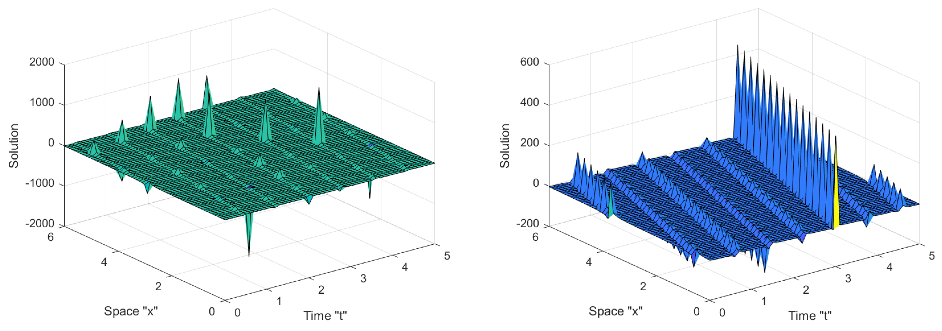
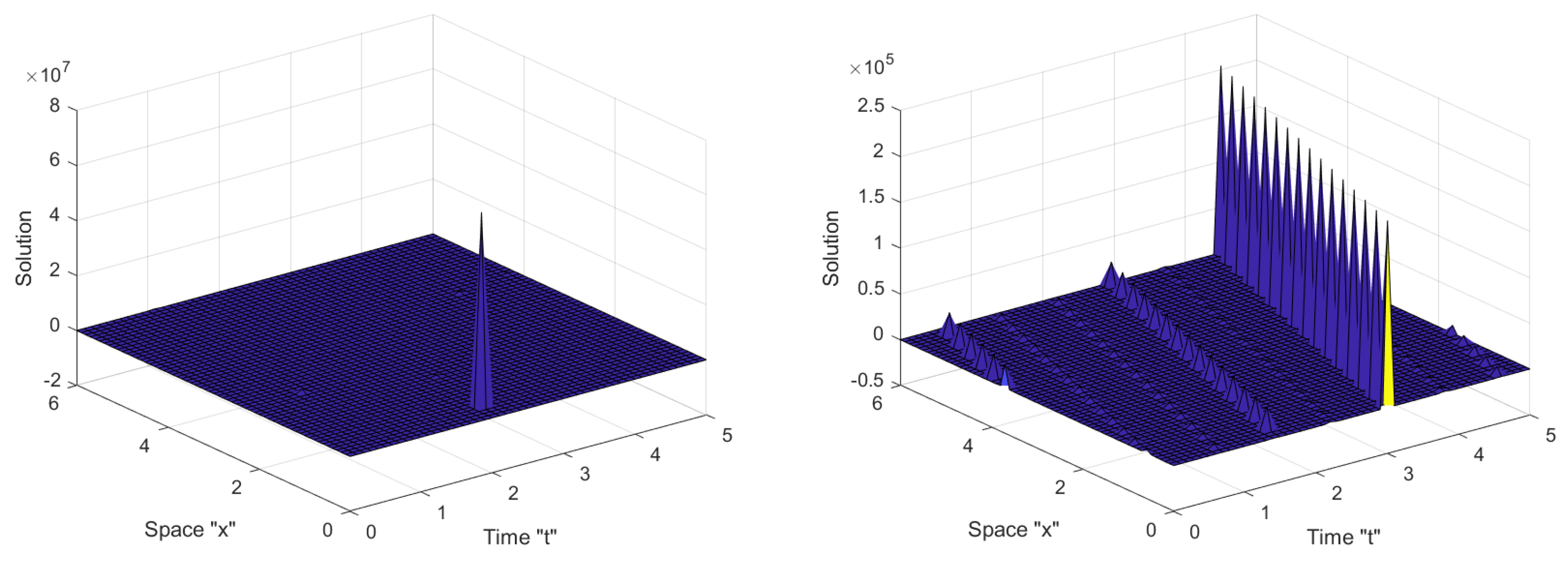
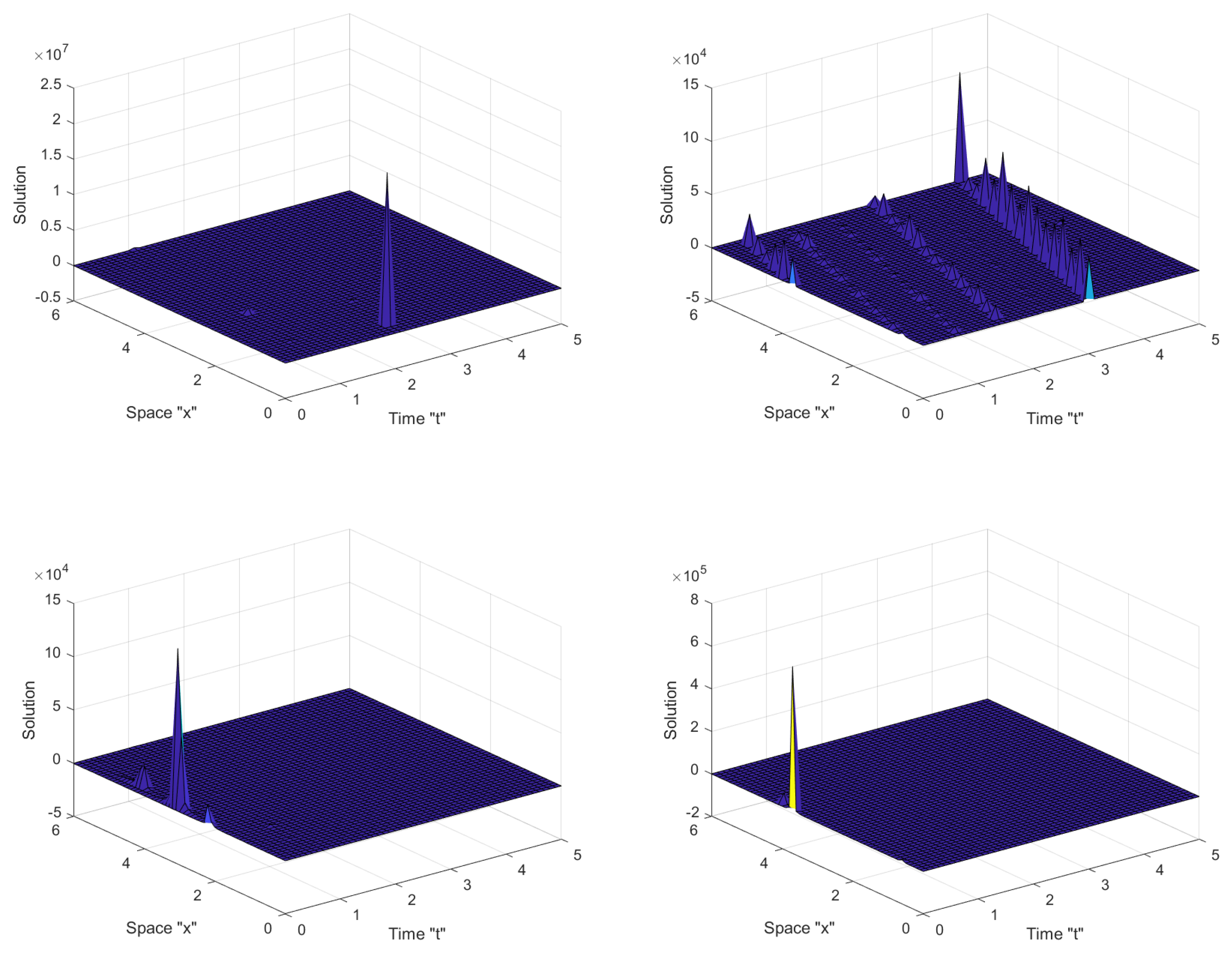
4. Analytical Solutions for SFSALWWE

We use here the Riccati equation method in order to find the solutions of Equation (13). Consequently, we acquire the analytical solutions of the SFSALWWE (Equations (1) and (2)). Initially, we suppose the solution of Equation (13) is

$$u=\sum _{i=1}^N{a}_i{\chi }^i,$$

(14)

where $\chi$ solves

$${\chi }^{\prime }={\chi }^2+\ell ,$$

(15)

where ℓ is a unknown constant. We note that Equation (15) has various types of solutions according to:

Family I: If $\ell =0,$ then

$$\chi \left(\eta \right)=\frac{-1}{\eta }.$$

(16)

Family II: If $\ell >0,$ then

$$\chi \left(\eta \right)=\sqrt{\ell }tan\left(\sqrt{\ell }\eta \right)\mathrm{or}\chi \left(\eta \right)=-\sqrt{\ell }cot\left(\sqrt{\ell }\eta \right).$$

(17)

Family III: If $\ell <0,$ then

$$\chi \left(\eta \right)=-\sqrt{-\ell }tanh\left(\sqrt{-\ell }\eta \right)\mathrm{or}\chi \left(\eta \right)=-\sqrt{-\ell }coth\left(\sqrt{-\ell }\eta \right).$$

(18)

Now, to determine the parameter N in Equation (14), we balance $u^3$ with $u^{″}$ in Equation (13) to get

$$N=1.$$

Rewriting Equation (14) with $N=1$ as

$$u=a_0+a_1\chi .$$

(19)

Differentiating Equation (19) twice, we have

$$u^{″}=2a_1\ell \chi +2a_1{\chi }^3.$$

(20)

Putting Equations (19) and (20) into Equation (13), we obtain

$$(2a_1-2a_1^3){\chi }^3-6(a_0{a}_1^2-\omega a_1^2){\chi }^2$$

$$-2(-a_1\ell +3a_0^2{a}_1-6\omega a_1{a}_0+2{\omega }^2{a}_1)\chi$$

$$-2(2a_0{\omega }^2-3\omega a_0^2+a_0^3)=0.$$

Equating each coefficient of ${\chi }^j$ to zero for $j=0,1,2,3$, we have

$$2a_0{\omega }^2-3\omega a_0^2+a_0^3=0,$$

$$-a_1\ell +3a_0^2{a}_1-6\omega a_1{a}_0+2{\omega }^2{a}_1=0,$$

$$a_0{a}_1^2-\omega a_1^2=0,$$

and

$$2a_1-2a_1^3=0.$$

Solving these equations, we obtain the next two sets:

$$\mathrm{Set}\mathrm{I}:a_0=\omega ,a_1=1,\ell =-\omega ,$$

(21)

and

$$\mathrm{Set}\mathrm{II}:a_0=\omega ,a_1=-1,\ell =-\omega .$$

(22)

For Set I: According to Equation (15), the solution of the traveling wave Equation (13) is

Family I-1: If $\ell =0$ (i.e., $\omega =0$), then

$$u_1\left(\eta \right)=\frac{1}{\eta }.$$

Using Equation (11), we obtain

$$v_1=-\frac{1}{{\eta }^2}.$$

Family II-1: If $\ell >0$(i.e., $\omega <0$), then

$$u_2\left(\eta \right)=\omega +\sqrt{-\omega }tan\left(\sqrt{-\omega }\eta \right).$$

Using Equation (11), we have

$$v_2=\frac{1}{2}{\omega }^2-\frac{1}{2}\omega .$$

Family III-1: If $\ell <0$(i.e.,$\omega >0$), then

$$u_2\left(\eta \right)=\omega -\sqrt{\omega }tanh\left(\sqrt{\omega }\eta \right).$$

Using Equation (11), we get

$$v_2=\frac{1}{2}{\omega }^2-\frac{1}{2}\omega .$$

Hence, the analytical solutions of the SFSALWWE (Equations (1) and (2)), respectively, are

$${\phi }_1(y,t)=\alpha y^{-\alpha }{e}^{(\rho \beta \left(t\right)-\frac{1}{2}{\rho }^{2}t)},$$

(23)

$${\psi }_1(y,t)=-{\alpha }^2{y}^{-2\alpha }{e}^{(\rho \beta \left(t\right)-\frac{1}{2}{\rho }^{2}t)},$$

(24)

$${\phi }_2(y,t)=[\omega +\sqrt{-\omega }tan(\frac{\sqrt{-\omega }}{\alpha }{y}^{\alpha }+\omega t)]e^{(\rho \beta \left(t\right)-\frac{1}{2}{\rho }^{2}t)},$$

(25)

$${\psi }_2(y,t)=(\frac{1}{2}{\omega }^2-\frac{1}{2}\omega +\omega t)e^{(\rho \beta \left(t\right)-\frac{1}{2}{\rho }^{2}t)},$$

(26)

and

$${\phi }_3(y,t)=[\omega -\sqrt{\omega }tanh(\frac{\sqrt{\omega }}{\alpha }{y}^{\alpha }+\omega t)]e^{(\rho \beta \left(t\right)-\frac{1}{2}{\rho }^{2}t)},$$

(27)

$${\psi }_3(y,t)=(\frac{1}{2}{\omega }^2-\frac{1}{2}\omega +\omega t)e^{(\rho \beta \left(t\right)-\frac{1}{2}{\rho }^{2}t)}.$$

(28)

For Set II (Equation (22)): According to Equation (15), the solutions of Equation (13) are:

Family I-2: If $\ell =0$ (i.e., $\omega =0$), then

$$u_4\left(\eta \right)=\frac{-1}{\eta }.$$

Using Equation (11), we obtain

$$v_4=0.$$

Family II-2: If $\ell >0$(i.e., $\omega <0$), then

$$u_5\left(\eta \right)=\omega -\sqrt{-\omega }tan\left(\sqrt{-\omega }\eta \right),$$

Using Equation (11), we have

$$v_5=\frac{1}{2}{\omega }^2+\frac{1}{2}\omega +\omega {tan}^2\left(\sqrt{-\omega }\eta \right).$$

Family III-2: If $\ell <0$(i.e.,$\omega >0$), then

$$u_6\left(\eta \right)=\omega +\sqrt{\omega }tanh\left(\sqrt{\omega }\eta \right).$$

Using Equation (11), we get

$$v_6=\frac{1}{2}{\omega }^2+\frac{1}{2}\omega -\omega {tanh}^2\left(\sqrt{\omega }\eta \right).$$

Hence, the analytical solution of the SFSALWWE (Equations (1) and (2)), respectively, are

$${\phi }_4(y,t)=-\alpha y^{-\alpha }{e}^{(\rho \beta \left(t\right)-\frac{1}{2}{\rho }^{2}t)},$$

(29)

$${\psi }_4(y,t)=0,$$

(30)

$${\phi }_5(y,t)=[\omega +\sqrt{-\omega }tan(\frac{\sqrt{-\omega }}{\alpha }{y}^{\alpha }+\omega t)]e^{(\rho \beta \left(t\right)-\frac{1}{2}{\rho }^{2}t)},$$

(31)

$${\psi }_5(y,t)=[\frac{1}{2}{\omega }^2+\frac{1}{2}\omega +\omega {tan}^2(\frac{\sqrt{-\omega }}{\alpha }{y}^{\alpha }+\omega t)]e^{(\rho \beta \left(t\right)-\frac{1}{2}{\rho }^{2}t)},$$

(32)

and

$${\phi }_6(y,t)=[\omega +\sqrt{\omega }tanh(\frac{\sqrt{\omega }}{\alpha }{y}^{\alpha }+\omega t)]e^{(\rho \beta \left(t\right)-\frac{1}{2}{\rho }^{2}t)},$$

(33)

$${\psi }_6(y,t)=[\frac{1}{2}{\omega }^2+\frac{1}{2}\omega -\omega {tanh}^2(\frac{\sqrt{\omega }}{\alpha }{y}^{\alpha }+\omega t)]e^{(\rho \beta \left(t\right)-\frac{1}{2}{\rho }^{2}t)}.$$

(34)

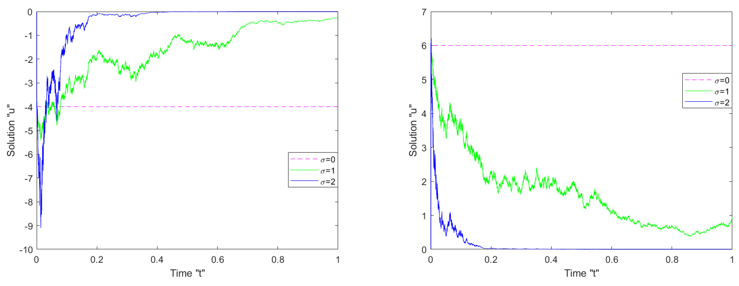
5. The Influence of Noise

In this manuscript, we investigate the effect of the noise term on the SFSALWWE (Equations (1) and (2)) solutions. To study the impact of multiplicative noise on these solutions, we employ MATLAB tools to display some graphs for various noise strength values. The solutions (31) and (32) for $y\in [0,6]$ and $t\in [0,5]$ are plotted below:

From Figure 1 and Figure 2: we see that the surface is not flat and that there is some irregularity.

From Figure 3 and Figure 4: we observe that after embedding noise and increasing its strength by $\sigma =1,2$, the surface becomes significantly flatter after minor transit patterns.

We can deduce from Figure 1, Figure 2, Figure 3, Figure 4 and Figure 5 below that the SFSALWWE (Equations (1) and (2)) solutions are affected by the multiplicative noise, which stabilizes them around zero.

6. Physical Interpretation

The deterministic approximate long water wave equation (i.e., (Equations (1) and (2)) with $\sigma =0)$ is used in hydrodynamics to explain the propagation of waves in dissipative and nonlinear media. When some external effect (random fluctuations) is considered, the behavior of these waves changes as shown in Figure 1, Figure 2, Figure 3 and Figure 4. As previously stated, external influences have an effect on the waves and cause them to become stable, as displayed in Figure 1, Figure 2, Figure 3 and Figure 4 with $\sigma \ne 0.$

7. Conclusions

We looked at the space-fractional stochastic approximate long-water-wave equation using conformable derivatives in this paper. The exact fractional stochastic solutions of the SFSALWWE (Equations (1) and (2)) were obtained via the Riccati equation method. These forms of solutions may be used for a broad range of curious and complicated physical phenomena because Equations (1) and (2) are widely utilized in ocean and coastal engineering; these forms are also advised for problems including water leakage in porous subsurface stratum. Further, these equations are also used in hydrodynamics to depict the propagation of waves in dissipative and nonlinear media. Finally, we showed how multiplicative noise affects solution behavior and concluded that the solutions of the SFSALWWE (Equations (1) and (2)) are stabilized around zero by multiplicative noise. We can use Equations (1) and (2) with additive noise or infinite dimension multiplicative noise in future research.

References

1. Prévöt, C.; Rxoxckner, M. A Concise Course on Stochastic Partial Differential Equations; Springer: Berlin/Heidelberg, Germany, 2007. [Google Scholar]
2. Mohammed, W.W.; Blömker, D. Fast diffusion limit for reaction-diffusion systems with stochastic Neumann boundary conditions. SIAM J. Math. Anal. 2016, 48, 3547–3578. [Google Scholar] [CrossRef] [Green Version]
3. Imkeller, P.; Monahan, A.H. Conceptual stochastic climate models. Stoch. Dynam. 2002, 2, 311–326. [Google Scholar] [CrossRef]
4. Zhou, Y.; Jiao, F.; Li, J. Existence and uniqueness for p-type fractional neutral differential equations. Nonlinear Anal. 2009, 71, 2724–2733. [Google Scholar] [CrossRef]
5. Deng, W. Smoothness and stability of the solutions for nonlinear fractional differential equations. Nonlinear Anal. 2010, 72, 1768–1777. [Google Scholar] [CrossRef]
6. Iqbal, N.; Yasmin, H.; Ali, A.; Bariq, A.; Al-Sawalha, M.M.; Mohammed, W.W. Numerical Methods for Fractional-Order Fornberg-Whitham Equations in the Sense of Atangana-Baleanu Derivative. J. Funct. Spaces 2021, 2021, 2197247. [Google Scholar] [CrossRef]
7. Iqbal, N.; Wu, R.; Mohammed, W.W. Pattern formation induced by fractional cross-diffusion in a 3-species food chain model with harvesting. Math. Comput. Simul. 2021, 188, 102–119. [Google Scholar] [CrossRef]
8. Shah, K.; Sher, M.; Ali, A.; Abdeljawad, T. On degree theory for non-monotone type fractional order delay differential equations. AIMS Math. 2021, 7, 9479–9492. [Google Scholar] [CrossRef]
9. Kamal, R.; Rahmat, G.; Shah, K. On the Numerical Approximation of Three-Dimensional Time Fractional Convection-Diffusion Equations. Math. Probl. Eng. 2021, 2021, 4640467. [Google Scholar]
10. El-Sayed, A.M.A.; Gaber, M. The Adomian decomposition method for solving partial differential equations of fractal order in finite domains. Phys. Lett. A 2006, 359, 175–182. [Google Scholar] [CrossRef]
11. Zhang, S.; Zhang, H.Q. Fractional sub-equation method and its applications to nonlinear fractional PDEs. Phys. Lett. A 2011, 375, 1069–1073. [Google Scholar] [CrossRef]
12. Guo, S.M.; Mei, L.Q.; Li, Y.; Sun, Y.F. The improved fractional sub-equation method and its applications to the space-time fractional differential equations in fluid mechanics. Phys. Lett. A 2012, 376, 407–411. [Google Scholar] [CrossRef]
13. Wang, M.L.; Li, X.Z.; Zhang, J.L. The ( G G )-expansion method and travelling wave solutions of nonlinear evolution equations in mathematical physics. Phys. Lett. A 2008, 372, 417–423. [Google Scholar] [CrossRef]
14. Wazwaz, A.M. A sine-cosine method for handling nonlinear wave equations. Math. Comput. Model. 2004, 40, 499–508. [Google Scholar] [CrossRef]
15. Mohammed, W.W. Approximate solutions for stochastic time-fractional reaction–diffusion equations with multiplicative noise. Chin. Ann. Math. Methods Appl. Sci. 2021, 44, 2140–2157. [Google Scholar] [CrossRef]
16. Mohammed, W.W. Modulation Equation for the Stochastic Swift–Hohenberg Equation with Cubic and Quintic Nonlinearities on the Real Line. Mathematics 2020, 6, 1217. [Google Scholar] [CrossRef] [Green Version]
17. Khan, K.; Akbar, M.A. The eyp(-ϕ(ς))-expansion method for finding travelling wave solutions of Vakhnenko-Parkes equation. Int. J. Dyn. Syst. Differ. Equ. 2014, 5, 72–83. [Google Scholar]
18. Malfliet, W.; Hereman, W. The tanh method. I. Exact solutions of nonlinear evolution and wave equations. Phys. Scr. 1996, 54, 563–568. [Google Scholar] [CrossRef]
19. Yang, X.F.; Deng, Z.C.; Wei, Y. A Riccati-Bernoulli sub-ODE method for nonlinear partial differential equations and its application. Adv. Diff. Equation 2015, 1, 117–133. [Google Scholar] [CrossRef] [Green Version]
20. Bulut, H.; Baskonus, H.M.; Pandir, Y. The Modified Trial Equation Method for Fractional Wave Equation and Time Fractional Generalized Burgers Equation. Abstr. Appl. Anal. 2013, 2013, 636802. [Google Scholar] [CrossRef]
21. Taghizadeh, N.; Mirzazadeh, M.; Rahimian, M.; Akbari, M. Application of the simplest equation method to some time-fractional partial differential equations. Ain Shams Eng. J. 2013, 4, 897–902. [Google Scholar] [CrossRef] [Green Version]
22. Ege, S.M.; Misirli, E. The modified Kudryashov method for solving some fractional-order nonlinear equations. Adv. Differ. Equ. 2014, 2014, 135. [Google Scholar] [CrossRef] [Green Version]
23. Al-Askar, F.M.; Mohammed, W.W.; Albalahi, A.M.; El-Morshedy, M. The Influence of Noise on the Solutions of Fractional Stochastic Bogoyavlenskii Equation. Fractal Fract. 2022, 6, 156. [Google Scholar] [CrossRef]
24. Al-Askar, F.M.; Mohammed, W.W.; Albalahi, A.M.; El-Morshedy, M. The Impact of the Wiener process on the analytical solutions of the stochastic (2+ 1)-dimensional breaking soliton equation by using tanh–coth method. Mathematics 2022, 10, 817. [Google Scholar] [CrossRef]
25. Albosaily, S.; Mohammed, W.W.; Hamza, A.E.; El-Morshedy, M.; Ahmad, H. The exact solutions of the stochastic fractional-space Allen—Cahn equation. Open Phys. 2022, 20, 23–29. [Google Scholar] [CrossRef]
26. Mohammed, W.W.; Iqbal, N.; Botmart, T. Additive Noise Effects on the Stabilization of Fractional-Space Diffusion Equation Solutions. Mathematics 2022, 10, 130. [Google Scholar] [CrossRef]
27. Mohammed, W.W.; Bazighifan, O.; Al-Sawalha, M.M.; Almatroud, A.O.; Aly, E.S. The Influence of Noise on the Exact Solutions of the Stochastic Fractional-Space Chiral Nonlinear Schrödinger Equation. Fractal Fract. 2021, 5, 262. [Google Scholar] [CrossRef]
28. Khalil, R.; Al Horani, M.; Yousef, A.; Sababheh, M. A new definition of fractional derivative. J. Comput. Appl. Math. 2014, 264, 65–70. [Google Scholar] [CrossRef]
29. Wang, M.L.; Zhang, J.L.; Li, X.Z. Application of the (G′/G)-expansion to travelling wave solutions of the Broer-Kaup and the approximate long water wave equations. Appl. Math. Comput. 2008, 206, 321–326. [Google Scholar] [CrossRef]
30. Guo, S.; Zhou, Y.; Zhao, C. The improved (G′/G)-expansion method and its applications to the Broer–Kaup equations and approximate long water wave equations. Appl. Math. Comput. 2010, 216, 1965–1971. [Google Scholar] [CrossRef]
31. Chen, Y.; Yu, Z. Generalized extended tanh-function method to construct new explicit exact solutions for the approximate equations for long water waves. Int. J. Mod. Phys. C 2003, 14, 601–611. [Google Scholar] [CrossRef] [Green Version]
32. Kaplan, M.; Akbulut, A. Application of two different algorithms to the approximate long water wave equation with conformable fractional derivative. Arab. J. Basic Appl. Sci. 2018, 25, 77–84. [Google Scholar] [CrossRef] [Green Version]
33. Yaslan, H.C. New analytic solutions of the space-time fractional Broer–Kaup and approximate long water wave equations. J. Ocean Eng. Sci. 2018, 3, 295–302. [Google Scholar] [CrossRef]
34. Yan, L. New travelling wave solutions for coupled fractional variant Boussinesq equation and approximate long water wave equation. Int. J. Num. Meth. Heat Fluid Flow 2015, 25, 33–40. [Google Scholar] [CrossRef]
35. Guner, O.; Atik, H.; Kayyrzhanovich, A.A. New exact solution for space-time fractional differential equations via (G′/G)-expansion method. Optik 2016, 130, 696–701. [Google Scholar] [CrossRef]
36. Khater, M.M.A.; Kumar, D. New exact solutions for the time fractional coupled Boussinesq-Burger equation and approximate long water wave equation in shallow water. J. Ocean. Eng. Sci. 2017, 2, 223–228. [Google Scholar] [CrossRef]
Figure 1. 3D shapes of the solution (31) for σ = 0 and α = 0.3 , 1 .
Symmetry 14 00740 g001
Figure 2. 3D shapes of the solution (32) for σ = 0 and α = 0.3 , 1 .
Symmetry 14 00740 g002
Figure 3. 3D shapes of the solution (31) for σ = 1 , 2 and α = 0.3 , 1 .
Symmetry 14 00740 g003
Figure 4. 3D shapes of the solution (32) for σ = 1 , 2 and α = 0.3 , 1 .
Symmetry 14 00740 g004
Figure 5. 2D shapes of the solutions (31) and (32) with α = 1 .
Symmetry 14 00740 g005
Publisher’s Note: MDPI stays neutral with regard to jurisdictional claims in published maps and institutional affiliations.